1. Introduction
With the development of society and the economy, the traditional manufacturing industry is facing dual pressures of rising land and labor costs, as well as competition in product prices. The material preparation stage in the production lifecycle of manufacturing products, namely the material storage stage, requires a large amount of labor, material resources, and factory area resources without generating any additional value. Therefore, there is an urgent need for cost reduction and efficiency improvement reforms. In this context, the Automated Storage and Retrieval System (AS/RS), based on key equipment such as high-rise shelves, stackers, and AGVs, has been promoted and applied in a wide range of industries due to its inherent advantages in storage capacity, unmanned degree, and operational efficiency. Especially for today’s manufacturing industry, which has just experienced the impact of the epidemic, researching the application of the AS/RS has important potential social security significance [
1].
As a typical labor-intensive industry, the introduction of the AS/RS for material storage is becoming an important trend for major shipyards to improve their material management level. The picking operation is the main business of the warehousing process, which usually accounts for more than 65% of the total workload. Therefore, research on order-picking optimization is one of the hot subproblems of AS/RS application problems, which has important practical significance, and this is no exception in the shipbuilding industry. However, it should be noted that the AS/RS order-picking problem in shipyards has its characteristics, as follows.
C1: Palletization is commonly used for the picking and usage of materials in shipyards. Palletization refers to the inherent set attribute of orders, and orders within the same pallet must be picked and outbound in the same batch. The efficiency of the operation is based on the overall picking time of the pallet.
C2: The processes of retrieving containers and picking the orders out from the containers to the pallet should be carried out simultaneously. The characteristics of small batch customized ship products determine that the AS/RS picking objects in the shipyard are many orders with significant differences. Therefore, pickers need the SKU (Stock Keeping Unit) numbers to assist in identifying during the order-picking process, which means the delayed order-picking strategies are not applicable in the shipyard AS/RS.
The above two characteristics indicate that the order-picking scheduling problem in the shipyard AS/RS is a complex scheduling problem that combines batch sorting of order groups and intragroup order-picking scheduling. Meanwhile, the tasks require multiple devices to complete. Especially under the conditions of multiple aisles, multiple picking stations, and multiple AGVs, this problem is more complex and difficult to solve than traditional order-picking problems. Its research has stronger practical significance and application value.
A large amount of research has been conducted on order-picking problems to optimize the operational efficiency of the AS/RS. Through relevant research reviews, the current research hotspots in order picking are gradually moving towards practical applications. Many mathematical models have been established for special scenarios in practical applications, as well as abundant optimization algorithms that consider a series of special elements such as different warehouse layouts, AGV power capacity limitations, order distribution routing problems, order conflict restrictions, etc. However, there are some shortcomings in existing research results, which have led to their inability to solve the AS/RS order-picking problems in shipyards. Most studies only consider single optimization objectives such as job efficiency or total order delay time, without simultaneously considering the dual demands of efficiency and cost [
2,
3,
4]. Furthermore, the majority of the literature has a different system composition from the shipyard AS/RS [
5,
6,
7,
8]. Meanwhile, most of them only focus on a single link of the whole main links, including stacker retrieval, order delivery, and order picking at picking stations, failing to achieve order-picking optimization in a multi-device collaborative mode [
9,
10]. Accordingly, the purpose of this paper is to solve the optimization problem of parallel order-picking scheduling in multi-device collaboration mode with the goal of reducing costs and increasing efficiency. This problem is named the Shipbuilding Automated Collaborative Order-picking (SACOP) problem in this paper.
The remainder of the paper is organized as follows:
Section 2 reviews the related literature.
Section 3 presents a description of the problem and proposes a method of the SACOP problem transformation.
Section 4 proposes a 0–1 integer programming model.
Section 5 gives the details of the INSGA-III-based MADPSO method. Computational results on numerous instances are reported in
Section 6. Conclusions and future research directions are suggested in
Section 7.
2. Related Work
As the core business of all types of warehouses, order picking has received widespread attention and research. According to the classification of the order-picking system [
11], the SACOP problem belongs to the manual picking problem of the parts to picker, so this review only focuses on the relevant literature of the parts-to-picker system. The system models of parts-to-picker systems can be divided into the AS/RS-based picking systems and Robotic Mobile Fulfillment Systems (RMFS). The main difference lies in the fact that the AS/RS-based picking systems use stackers or shuttle cars to retrieve the containers while RMFS sends the entire shelves to the picking stations by the mobile robots. To meet the needs of storage area, operational efficiency, energy consumption, and labor intensity, the AS/RS-based picking system in shipyards usually adopts a hybrid system composed of stackers, AGVs, and manual picking stations. Based on this, the SACOP problem can be decomposed into subproblems such as stacker scheduling, AGV delivery task scheduling, order batch, and sorting. Currently, there is little literature that uses this system to research the order-picking problem, which means existing research cannot be cited separately to solve the practical SACOP problem. Based on the above considerations, this paper comprehensively reviews the relevant literature on stacker scheduling, AGV task scheduling, RMFS order batch, and sort scheduling, as well as other relevant scenarios that are beneficial to this study. On this basis, the SACOP problem was proposed and studied.
2.1. Stacker Scheduling
Bozer et al. first constructed mathematical models for the expected walking time of stackers in single instruction mode and dual instruction mode in 1982 [
12]. Hwang et al. added stacker acceleration and deceleration as well as maximum driving speed on this basis [
13]. Subsequently, researchers gradually expanded the scheduling problem of stackers from single-station stackers to multi-stations stackers, from single stacker in single aisles to multi-stackers in single aisles [
14,
15,
16,
17], and from single deep to compact shelves. Under these special constraints, they studied sub problems such as stacker job scheduling, standby strategy, and path planning [
18]. By reviewing the above literature, the sorting of inbound and outbound tasks and the arrival interval between tasks have significant impacts on the efficiency and energy consumption of the stacker system. Therefore, it is necessary to consider the energy consumption and order delay performance of the stacker system under different order allocation decisions when discussing the SACOP problem.
2.2. AGV Task Scheduling
In the broad context, not only including shipyards, AGV scheduling optimization has been discussed extensively, which typically includes goals such as total delivery time or total delayed arrival time, path planning length, path conflict penalty, number of AGVs, energy consumption [
19,
20,
21], etc. For example, Nitish Singh et al. discussed the AGV scheduling problem under battery capacity constraints, with the optimization objective of minimizing AGV transportation time and the weighted total cost of order delay penalty [
22]. They established a mixed integer linear programming model for this problem and proposed an adaptive large neighborhood search algorithm as a solution. Xueting He et al. established a mixed integer programming model for waste, AGV, and picking station points allocation problems in medical waste sorting systems, and proposed a dynamic programming-based variable neighborhood search algorithm to solve practical problems [
23]. Although there are significant differences between the AGV scheduling literature reviewed above and the SACOP problem system model in this paper, the discussion and construction of models related to energy consumption and path conflict issues have great inspiration for this paper.
2.3. RMFS Orders Batch-Picking Scheduling
RMFS has been a popular picking system in recent years, which decomposes traditional warehouse picking activities into two sub-activities: handling by robots and picking by humans. This allows robots and manual pickers to complement each other’s advantages, freeing manual pickers from heavy handling activities while fully retaining and leveraging the experiential advantages of manual pickers in picking activities.
Azadeh et al. [
24] and Boysen et al. [
25] found that the order-picking problem in RMFS has not been fully resolved. Xiying Yang et al. [
26] paid attention to the coupling relationship between order sorting and mobile shelf scheduling. They established an integer programming model to describe the problem and proposed a two-stage solution method to solve the joint optimization of order sequencing and mobile shelves scheduling. Zhang, Jingtian et al. [
27] innovatively transformed the robot task scheduling problem into a resource-constrained project scheduling problem with transfer time and proposed a genetic algorithm using a building-block-based crossover (BBX) operator to solve this problem. Justkowiak et al. [
28] also recognized the correlation between order sorting and shelf scheduling and proposed a new mixed integer programming formula based on original preprocessing techniques to solve the order and shelf sorting problem with a single picking station, which provided a reference example for the optimization problem of RMFS orders at a medium scale. Teck and Dewil [
29] established an integrated order scheduling model that differs from the commonly used phased decision-making model in other literature and proposed a heuristic solution method called a bi-level psychological memetic algorithm, which further extended the two problems of order sorting and shelf scheduling. In addition, Amir Gharehgozli et al. [
30] first incorporated the recycling of pods into the RMFS order-picking model. The process of pod picking and recycling described in the model is like the order recycling in the SACOP problem. However, the model proposed in that paper was limited by a single picking station and considered the single optimization objective, which was unsuitable for the SACOP problem.
By reviewing the literature mentioned above, although there are certain differences in the order-picking system (OPS) between RMFS and SACOP, based on similar behavior patterns and related constraints, the mobile shelves in RMFS can be considered AGVs to some extent in the SACOP problem. Therefore, summarizing the above literature can further clarify the strong coupling between order batch picking and AGV scheduling in the SACOP problem. The relevant ideas, mathematical models, and optimization algorithms design have significant inspiration for the study in this paper. In addition, the literature [
31] on the labor intensity of picking workers provides useful insights for this paper, and the literature [
32,
33] provided useful optimization method design ideas for this paper.
By the literature review in this section, the limitations of existing research have been clarified: (1) There is a lack of research on collaborate picking systems’ concluding stackers, AGVs, and picking stations. (2) Existing research has overlooked other important optimization objectives, such as machine energy consumption and worker load, or subjectively weighted multiple optimization objectives into a single objective, which resulted in the results deviating from reality. On the other hand, this also demonstrates the complexity of the SACOP problem.
As a result, this paper dictates the multi-objective scheduling optimization model and method for the SACOP problem, firstly, which takes the overall energy consumption and operational efficiency into account. With our work, a Pareto optimal solution set can be generated within a reasonable time range for a batch outbound task of orders and transformed into corresponding stacker scheduling schemes, AGV scheduling schemes, and pick station task schemes.
3. System Specification
3.1. System Composition
The AS/RS-based picking system structure discussed in this paper includes three parts: storage unit, transport unit, and picking unit. The detailed system composition is shown in
Figure 1.
The storage unit consists of high-rise shelves and stackers. In the AS/RS discussed in this paper, the high-rise shelves provide sufficient storage compartments, and each compartment can store a standard container. Each container, as a SKU, usually stores multi-shipbuilding material items with separate material identification codes, and the orders to pick in the task are included in these materials. The stackers of storage units referred to in this paper are the most common medium-sized double-column stackers. One stacker is arranged in one aisle and each stacker is responsible for the storage and retrieval of containers. The handover points between the stackers and AGVs are set at the exit of the aisles.
The transport unit consists of multiple AGVs of the same model. When the AGVs are idle, they can be on standby or charged in the designated charging area.
The picking unit includes multiple picking stations with workers for parallel operations, each of which is managed by a picking worker. Considering the space limitations of the picking station, as well as the difficulty and probability of errors for workers, this paper sets an upper limit of three pallets that can be picked simultaneously at each picking station.
3.2. SACOP Process
In addition to the system composition, we will further explain the system process. The research object of the SACOP problem is the pallet-picking task in the shipyard AS/RS. It is easy to confuse that the concepts of “pallet” and “order” mentioned in this paper differ from the traditional OPS literature. Therefore, a brief explanation of these two concepts will be provided first. Palletized material management is an important means to support modern shipbuilding. The original meaning of a “pallet” is the container that carries sorted materials, and it is also used to refer to this batch of materials on the pallet in shipyard material management. This paper will continue to use this material management concept, using the “pallet” to refer to the set of sorted materials and using the “order” to refer to each specific material contained in the pallet.
The main process of pallet picking is shown in
Figure 2. Firstly, the pallet-picking tasks are assigned to each picking station, and the picking station will open several pallet-picking tasks based on its own capacity limit. After the tasks are opened, the upstream storage unit will “spit out” the containers to which the orders belong. The containers spit out are transported by AGVs to the picking stations to pick out. After all orders in the pallet are picked out, close the pallet-picking task, and open a new one until all pallet-picking tasks are completed.
The pallet-picking task consists of basic order-picking cycles. As shown in
Figure 3, the operation cycle of a single order includes three stages, extracting the container, transporting the container, and returning the container, as well as two interactive nodes: handing over the container between the stacker and AGV, and AGV waiting at the picking station for the order to be picked out.
During the entire SACOP operation process, each device needs to interact with other devices for each operation, which will have a profound impact on itself and the entire system. Therefore, solving the SACOP optimization problem is extremely difficult. Due to the lack of a multi-devices collaborative scheduling solution, current shipyards adopt a picker-led mode for pallet picking in the shipyard AS/RS, which can be referred to as the traditional pallet-picking mode (TPPM), as shown in
Figure 4.
3.3. Transformation of SACOP
Considering the strong coupling relationship between various devices in the SACOP environment, it is extremely difficult to simultaneously schedule stackers, AGVs, and picking stations to operate without conflicts and achieve energy consumption and operation efficiency optimization goals. Furthermore, even if there is a set of optimized collaborative solutions, they have almost no anti-interference ability in the face of various uncertain factors in actual operations. Based on the above understanding and inspired by TPPM, this paper proposes an approach to find a key device to dominate the entire scheduling process and ensure that it can be transformed into a collaborative scheduling solution. Due to the ability of AGVs to connect upstream and downstream units in the system, their scheduling schemes have the potential to drive stackers and picking stations to operate. Therefore, this paper chooses them as key devices, thereby transforming the original SACOP problem into a modified multi-AGV scheduling task problem (MMATSP), as shown in
Figure 5.
The modifications of the MMATSP mainly include two aspects, which correspond to the interaction strategy of stacker, AGV, and the interaction strategy of picking station, AGV: one is that the stacker subsystem will perform pickup waiting correction on the original solution, and the other is that the picking station subsystem will perform waiting correction caused by capacity limit.
Interaction strategy of stacker, AGV: Due to the maximum driving speed and the ideal driving speed with the lowest energy consumption of the stacker, there is a “minimum time”, represented by , and an “ideal time”, represented by , for the extraction process of each container. We refer to the time between the moment when the previous AGV leaves the aisle and the moment when the next AGV arrives at the aisle as the “demand time” for this container, represented by . The stacker subsystem adopts the following operating strategy: for , operate at the ideal driving speed; for , operate at the specified speed to ensure synchronized container handover with the AGV; and for , operate at the rated maximum speed to reduce the waiting time of the AGV.
Interaction strategy of picking station, AGV: Waiting correction caused by capacity limit refers to the need for the AGV delivery to consider the capacity limit of the picking station. When an AGV arrives at the picking station, if the pallet containing this order is open or if the picking station capacity does not reach the upper limit, then the delivery is completed; if the order does not belong to any pallet being operated and the picking station capacity reaches the upper limit, then wait for the picking station capacity to be released. Due to the possibility of system deadlock caused by AGVs on standby waiting, standby waiting is modified to set up a temporary store buffer to wait for the capacity release in this paper, which is called buffer waiting. An example of a system deadlock is shown in
Figure 6. When using the buffer waiting strategy, orders that need to wait are directly sent to the buffer, while the AGV continues to perform subsequent tasks. When the picking station capacity is released, the original AGV picks up the order from the buffer and sends the container to the picking station. Compared to standby waiting, the buffer waiting strategy increases the construction cost of the buffer and incurs additional energy consumption for AGV’s round-trip to and from the buffer. However, on the one hand, it can enable AGVs to quickly carry out subsequent order tasks, thereby improving overall efficiency. On the other hand, it converts standby waiting time into AGV’s round-trip time, which is equivalent to exchanging energy consumption for efficiency considering the first advantage. For the same solution as the MMATSP, these two strategies have similar comprehensive indicators of energy and efficiency, so using a buffer waiting strategy instead of a standby waiting strategy is reasonable. The last and most important is that the buffer waiting strategy ensures that each AGV scheduling scheme is a feasible solution. The pallet-picking process after adopting the MMATSP is shown in
Figure 7.
3.4. Problem Definition
Finally, we define the SACOP problem as pallet-picking tasks that need to be assigned to picking stations, while each pallet contains several orders, and a maximum of pallets can be picked simultaneously at each picking station. Only the pallets with all orders picked up can leave the picking table. The materials corresponding to orders in the pallets are stored in containers, while . The containers are stored on high-rise shelves and need to be taken out by stackers and transported to the picking stations by a maximum of single-load AGVs. It is needed to find the optimal decision-making solution that minimizes the total operation time and minimizes system energy consumption.
4. Mathematical Model
4.1. Assumption
Before further research on the problem, to facilitate the research of the problem and the establishment of the model, the following assumptions are made:
When orders within the same pallet belong to the same container, these orders are considered as one consolidated order.
Once the pallet-picking task is opened, it can only be closed when all the associated orders are completed.
There is a limit to the number of pallets that can be picked simultaneously by each picking station, and this paper assumes it to be three.
The operation time for actions such as retrieving containers, handing over containers, and picking out orders is not considered.
The stacker is a single load and can only retrieve one container at a time.
The stacker is assumed to drive at a constant speed, without considering the acceleration and deceleration process. Its constant lifting and lowering speed are expressed as , the maximum horizontal speed is expressed as , and the ideal horizontal movement speed with the best energy consumption is expressed as .
Each handover point at the aisle port can only store up to one container.
AGV is a single-load vehicle that can only transport one container at a time and drives at a constant speed along a straight line at a speed of 1 m/s without considering acceleration and deceleration processes.
AGVs adopt the predetermined acceleration and deceleration strategy to avoid collisions, with the same additional energy consumption paid each time.
The power limit of AGVs and the capacity limit of the buffer zone are not considered.
4.2. Solution Expression
In
Section 3.3, we propose an approach to transform optimal collaborative scheduling for the SACOP into the optimal AGV scheduling for the MMATSP. In this paper, the SACOP optimal collaborative scheduling scheme is referred to as the executable solution, and the MMATSP optimal AGV scheduling scheme is referred to as the direct solution. According to the previous description, the executable solution can be obtained through simulation calculation of the direct solution. For a clearer expression, we use
to represent the direct solution, use
to represent the executable solution, and use
to represent the process of obtaining the executable solution through simulation calculation of the direct solution, where the function
represents the simulation calculation method.
As shown in Equation (1),
is a direct solution expressed jointly by two
matrices
and
, where
represents the number of available AGVs and
represents the total number of order tasks. Corresponding to the intuitive expression of AGV task sequences, the order task sequences of
AGVs are obtained by removing zero elements from
row vectors extracted from matrices.
Among them:
represents the order number of task of AGV ;
represents the picking station number of task of AGV ;
The decision variable is equal to one, iff order is assigned as task of the AGV ; otherwise, it is equal to zero;
The decision variable is equal to one, iff order is assigned to picking station ; otherwise, it is equal to zero.
The converted through function is divided into three parts: stacker scheduling scheme , AGV scheduling scheme , and picking station scheduling scheme .
Among them:
includes a list of retrieval tasks for each stacker, and each individual instruction of retrieval task
for stacker
includes three parts: container number
, AGV pickup time
, and stacker driving speed
, as shown in Equation (2).
is the AGV running trajectory list that includes order numbers, node location information, and node entry–departure time, as shown in Equation (3).
The picking station scheduling scheme
is an arrival information table that includes the order number, the pallet number to which the order belongs, and the delivery time of the order, as shown in Equation (4).
4.3. Objective Function
The objectives of the SACOP problem can be divided into three functions, , , and , in which represents the aim of minimizing energy consumption of the stacker subsystem, represents the aim of minimizing energy consumption of AGV subsystem, and represents the aim of minimizing system operation time.
4.3.1. Stacker Energy Consumption Objective
In the context of this paper, different AGV scheduling schemes determine different horizontal driving speeds of stackers. Therefore, before giving the expression for , it is necessary to first clarify the relationship between the energy consumption of a single operation of the stacker and the horizontal driving speed of that operation.
Firstly, we provide a simple Inference 1 directly without proof:
Inference 1. The energy consumption difference of a stacker completing the same task at different speeds is directly proportional to the difference in the square of the horizontal driving speed.
When we release the constraint of the demand time window for stacker retrieval tasks, there must be a unique minimum operating energy consumption of the stacker subsystem for each direct solution. Therefore, we can use the difference between the actual energy consumption and the theoretical minimum energy consumption to characterize the stacker energy consumption objective. Furthermore, we provide the final expression for
based on Inference 1, as shown in Equation (5).
represents the value of the horizontal driving speed of stacker to retrieve task , and represents the unit objective function value of stacker to retrieve task .
Since the waiting time for AGV pickup is determined by an external factor, the operating strategy of the stacker is necessary to provide an exact calculation method for to ensure the computability of function . The calculation method for is shown as follows.
Firstly, we let be the -th retrieved container of the stacker , where represents the handover completed time of , and represents the arrival time of the AGV picking up . Meanwhile, represents the overall time for retrieving , and represents demand time for task . In addition, let represent the waiting time for AGV to pick up container .
For each container
, its inherent storage location attribute corresponds to three inherent time attributes, as shown in Equations (6)–(8), in which
represents theoretical optimal operation time,
represents the minimum operation time considering the horizontal movement speed limit,
represents the minimum operation time considering vertical movement speed limit,
represents the horizontal coordinates of the
storage location, and
represents the vertical coordinates of the
storage location.
On the premise of fully discussing all possible size relationships among
, we provide a calculation method for
, as shown in Equation (9), and an update method of
that supports iteration, as shown in Equation (10).
4.3.2. AGV Energy Consumption Objective
In the SACOP problem, the total driving energy consumption of AGVs is mainly affected by two non-negligible factors: the total length of the AGV path and the number of path conflicts. Under the condition of constant speed and conflict-free driving, the energy consumption of AGV is directly proportional to the path length. However, there are often collision conflicts between the multi-AGV driving paths determined by direct solutions. Considering that the AGV operating space in the SACOP problem is a free rectangular plane, rather than the aisle environment with finite degrees of freedom in traditional problems, adopting a speed control strategy to avoid conflicts is the most economical and feasible method. By adding a mirrored acceleration–deceleration process at possible conflict points, collisions can be avoided while also avoiding any impact on the system scheduling plan. Under a unified speed control strategy, the speed adjustment energy consumption of AGVs to avoid conflicts can be seen as directly proportional to the number of conflicts.
To sum up, the minimum AGV energy consumption objective function
can be expressed as Equation (11).
represents the total length of the driving path of AGV , represents the number of conflicts that occurred by AGV , and is the conversion coefficient related to the system, which can be measured experimentally for specific systems.
4.3.3. System Operation Time Objective
According to the relevant description in the solution expression section, the completion moment of the latest completed AGV is the final completion moment of all pallet-picking tasks for this round. Based on this, we provide the expression of
, as shown in Equation (12).
represents the termination time of each AGV and represents the start time of each AGV.
4.4. Constraint
This problem includes several conventional constraints (Constraint 1, 2, 4) and a special constraint (Constraint 3).
Constraint 1 is expressed as follows: each order should be picked and only picked once, which can be guaranteed by Equations (13) and (14).
Constraint 2 is expressed as follows: the usage of the device cannot exceed its available limit, which can be guaranteed by Equations (15) and (16).
Constraint 3 is expressed as follows: the orders belonging to the same pallet can only be picked by the same picking station.
To mathematically express Constraint 3, we first define a function
to represent the subordination relationship between pallet
and order
, which is equal to one iff the order
belongs to the pallet
. Next, we structure a matrix
as shown in Equation (17). Finally, the matrix
is constrained by Equation (18) to ensure that Constraint 3 holds.
Constraint 4 is expressed as follows: pallet-picking tasks that are simultaneously open on the picking station cannot exceed the upper capacity limit of the picking station.
Due to each order belonging to a unique pallet, the picking operation time window for each pallet can be obtained based on the order arrival schedule of each picking station as described in
Section 4.2. We use
to represent the picking operation time interval of pallet
on picking station
, use
to represent the upper limit of the picking station capacity, and use
to represent the set
. When
, we use
to represent any subset of
with a size of
. To sum up, Constraint 4 can be guaranteed by Equation (19):
5. MADPSO Method Design
Due to the lack of a unified mathematical expression for the function , it is not enough to solve the SACOP problem relying solely on the mathematical model. Thus, this paper proposes a multi-AGV-driven pallet-picking scheduling optimization (MADPSO) method based on the improved NSGA-III to solve the SACOP problem.
The Non-dominated Sorting Genetic Algorithm III (NSGA-III) was proposed by Kalyanmoy Deb in 2014 [
34], which includes main steps such as population initialization, crossover, mutation, and non-dominated sorting selection. Due to the introduction of an elite preservation strategy and selection operator based on the reference point, it has outstanding convergence speed and population diversity advantages in solving multi-objective optimization problems and is currently one of the most efficient algorithms.
Based on the characteristics of the SACOP problem, this paper has specially designed and improved the chromosome encoding, chromosome decoding, crossover, and mutation operators in the original NSGA-III. The process of using the function for solution transformation is designed as a specific decoding process.
In addition, decision makers usually need a few candidate solutions, and they may have different energy consumption and efficiency tendencies in different situations. This means that the Pareto solution set provided by the traditional NSGA-III cannot directly meet the decision-making needs. In this regard, this paper specifically introduces the multi-objective decision-support operator TOPSIS (Technique for Order Performance by Similarity to Ideal Solution) [
35]. On the one hand, this operator can perform decision-support ranking on the Pareto front to assist in making final decisions, and on the other hand, it can label the decision-support optimal individuals in each generation of the population as auxiliary reference points to verify the convergence of the algorithm.
5.1. General Procedure of MADPSO
The main process of MADPSO based on INSGA-III is shown as the pseudocode of Algorithm 1, which includes the following steps:
Step 1: Initialize population. Based on the input system parameters (system component coordinates, capacity of the picking station, container coordinates, containers’ dependent orders set, etc.), as well as the corresponding problem parameters (pallet-picking tasks set, the used picking station numbers, available AGV quantities, etc.), individuals are generated randomly to form the initial population .
Step 2: Generate offspring by crossover operator. individuals are generated by performing the crossover operator designed in this paper on the current parent population to form an offspring population .
Step 3: Merge to generate a mixed population. Combine the parent population obtained in the previous step and the offspring population into a new population , which can be expressed as .
Step 4: Perform mutation operators. Perform mutation operations on each individual in the mixed offspring to update .
Step 5: Perform non-dominated sorting on . Calculate the fitness function of each individual in and non-dominated sort based on it, thereby marking the dominance level of each individual.
Step 6: Select the next-generation population from . Starting from the layer, individuals are selected from layer by layer and placed in the next-generation population according to the dominance level, which continues until the number of individuals in the layer is greater than the remaining demand individuals of the next-generation population. Afterwards, select individuals closest to the nearest reference point from the layer to thereby make up for the missing individuals in .
Step 7: Perform decision-support sorting operator on . Sort the individuals in by the TOPSIS method and label the most prioritized individual among them.
Step 8: Repeat Step 2–Step 7 until the predetermined number of iterations is reached and output the individuals in the layer of the last-generation population as the Pareto solution set. At the same time, output the decision-support solution labeled by the TOPSIS operator.
| Algorithm 1: MADPSO method general procedure |
| Input: system parameters (system component coordinates, capacity of the picking station, container coordinates, containers’ dependent orders set, etc.), problem parameters (pallet-picking tasks set, the used picking station numbers, available AGV quantities, etc.), population size , maximum number of iterations . |
| Output: Pareto solution set , decision-support solution . |
1. Initial population ,
2. While do
3.
4.
5.
6.
7. , , and
8. while do
9.
10.
11.
12. end while
13.
14.
15.
16.
17. end while
Get the set of as the Pareto solution set |
| Return, |
5.2. Algorithm Design
This subsection will introduce the details of the encoding, decoding, crossover, mutation, selection, and TOPSIS operators designed in the MADPSO method.
Specifically, in order to ensure population diversity and global search ability during the evolution process of the algorithm, thereby avoiding falling into local optima, the MADPSO method has specially designed a layered crossover strategy and set independent mutation rates and strategies for different chromosome segments. Furthermore, the parent population preservation strategy and reference-point-based individual selection method that are beneficial for maintaining population diversity in the NSGA-III were also adopted. In addition, the MADPSO method also designed an effective stopping criterion to determine the termination condition of the algorithm. This criterion can be understood as a termination criterion for algorithms based on the convergence necessity criteria of the reference evolution curve obtained by the TOPSIS operator and the number of individuals in the top priority non-dominated layer, combined with the maximum iteration limit.
5.2.1. Chromosome Coding
In response to the need to arrange the picking station and the AGV for each order simultaneously in the SACOP problem, we designed a double-layer integer encoded chromosome, and a specific example of the chromosome structure is shown in
Figure 8.
The first layer of chromosomes represents the allocation of pallet-picking tasks for each picking station, which is named the Picking Station Task-allocation Layer. The gene value of the gene represents the allocation of pallet to picking station .
The second layer of chromosomes represents the order-task sequence of each used AGV, which is named the AGV Task-allocation Layer. Referring to the example in
Figure 8,
,
, etc., represent the AGV numbers called in this solving process. We refer to these genes as AGV Genes, while the remaining genes are referred to as Order Genes. The Order Gene string is cleaved into several Order Gene sub-strings by the AGV Genes, and each Order Gene sub-string represents a task sequence fragment belonging to its head AGV Gene. The final task sequences of each AGV can be obtained by concatenating the Order Gene sub-strings belonging to the same AGV successively.
In addition, to facilitate the random generation of the initial population, we adopt the following method to generate the AGV Task-allocation Layer chromosome: first, all orders are randomly sorted to an initial sequence, then several breakpoints are randomly generated in the initial sequence (there will always be a breakpoint on the first gene locus), and, finally, each breakpoint is randomly assigned an available AGV number.
5.2.2. Queuing Service Model-Based Decoding Operator
As mentioned above, SACOP is a parallel tasks’ collaborative scheduling problem with the coupled temporal relationship, while the designed chromosome code only contains the task allocation and sequence of each AGV, which means the decoding operator is a process to complete the AGV task timing information. However, due to the complexity of the parallel tasks’ temporal problem, it is difficult to give a few formulas to complete the decoding process. Moreover, the measure mentioned above to ensure that all solutions are feasible by setting a buffer zone may also lead to the inconsistency between the real task execution order of AGV and the encoding information, which further increases the difficulty of decoding by direct calculation. Therefore, it is necessary to find a new decoding method.
Considering that in the two working states of AGV static operation and dynamic traveling, the AGV in the dynamic phase will not change the temporal state of the current system until it reaches the next endpoint (static operation point), and we can convert the decoding process into a special queuing service model (as shown in
Figure 9). In the model, multiple parallel AGV tasks’ sequences converge into a single temporal workflow through a temporal information-adding window. Based on the above cognition, this paper proposes a simulation decoding method based on the queuing service model.
The main flow of the decoding operator is shown in the following steps:
Step 1: Generate task sequences for each AGV based on individual chromosome information, where represents the -th task’s order number, represents the -th task’s picking station number, and represents the -th task’s stage (including pick up, delivery, and container return).
Step 2: Check the status of picking stations and move the buffered orders contained in the pallets that are being picked to the corresponding task sequence header of the AGV.
Step 3: Take the first tasks in each AGV task sequence to form the set to be served and calculate the to-be-served tasks’ time of arrival in endpoints (in particular, we take a large value for the endpoint arrival time of the pickup task of the occupied container to indicate that it has the lowest priority to be served).
Step 4: Take the task with the earliest arrival time in the to-be-served set as the service object this time and check its task stage. If the stage is picking up, skip to Step 5; if it is delivering, skip to Step 6; and if it is container return, skip to Step 7.
Step 5: Calculate the endpoint departure time and the stacker energy consumption of the task, update the container status to “occupied”, and update the task phase information to “delivery”. When finished, skip to Step 8.
Step 6: Check the picking pallet information of the picking station to determine whether the order can be picked. If the order can be picked out, the following process is performed in sequence: check the remaining orders in the container that can be picked out, update the AGV task sequence, add the endpoint departure time of this task, update the task phase information to “container return”, and update the container destination according to the number of remaining orders in the container. If the order cannot be picked out, the following process shall be performed in sequence: check the remaining orders that can be picked out in the container, update the AGV task sequence, add the order task to the buffer task sequence, add the endpoint departure time of this task, update the task stage information to “container return”, and update the container return destination to “buffer”. When finished, skip to Step 8.
Step 7: Execute the following process in sequence. Add the endpoint departure time of the task; update the container status to “available”; delete the first task in the corresponding AGV task list. When finished, skip to Step 8.
Step 8: Update the track list of the AGV corresponding to the service object and update the total energy consumption of the stacker system.
Step 9: Check whether all orders have been picked. If yes, go to Step 10. If no, go to Step 2.
Step 10: Calculate and output the individual’s fitness values .
5.2.3. Fitness Function
Based on the description in the mathematical model section, the fitness function of the MADPSO method is also divided into three types: stacker energy consumption , AGV energy consumption , and total operation time .
By performing the designed decoding operator, the energy consumption of each stacker during each operation and the trajectory matrix of all AGVs corresponding to each chromosome individual can be obtained. By accumulating the energy consumption of a single operation of the stacker, the total energy consumption of the stackers can be obtained. The trajectory matrix carries the position and time information of the entire AGV operation process, and through these trajectory matrices, a public solution space can be constructed.
As shown in
Figure 10, for a specific individual’s corresponding public solution space, the total length of each AGV trajectory projected on the
plane is the total length of the AGVs’ travel path. By designing a reasonable step size to discretize the
-axis to check the projection layer by layer, the total number of conflicts between AGVs can be obtained. Quoting Equation (9) can obtain the energy consumption
of AGVs. In addition, the difference between the maximum and minimum values of the projections of each AGV trajectory in the
-axis direction is the total system operation time
of the individual.
5.2.4. Crossover Operator
Since conventional crossover operators are not suitable for the double-layer integer encoded chromosome in this paper, we designed a segmented crossover operator, which includes two parts: perform double-point crossover at the Picking Station Task-allocation Layer and perform single-point crossover at the AGV Task-allocation Layer.
As shown in
Figure 11,
and
represent the Picking Station Task-allocation Layer chromosomes of two-parent individuals, and the double-point crossover is performed by exchanging chromosome fragments between two randomly selected genes. Due to the simple encoding form in the Picking Station Task-allocation Layer and the independent between information of different genes, using double-point crossover helps to expand the search range of the algorithm.
Because the genetic information of the AGV Task-allocation Layer is jointly expressed by AGV Genes and Order Genes, and individual genes do not have complete independence in genetic information expression, we adopt a less destructive single-point crossover method. The crossover process of the AGV Task-allocation Layer is divided into two steps: Order Gene crossover and AGV Gene crossover, and a specific example is shown in
Figure 12.
5.2.5. Mutation Operator
Since different types of segments in the double-layer chromosome have different gene expression patterns, it is necessary to separately design mutation modes and probabilities for different parts. After multiple tests and adjustments, this paper uses a vector to represent the probability of mutation, which includes the mutation rate of 0.04 in the Picking Station Task-allocation Layer, 0.2 in the Order Gene, and 0.16 in the AGV Gene.
Different parts of chromosomes correspond to different modes of mutation. For the Picking Station Task-allocation Layer chromosome, traverse each gene for mutation detection, and when a gene mutates, replace the value of that gene with any other available value. The mutation of AGV Gene and Order Gene occurs at the individual level. For AGV Genes, when an individual mutates, select an AGV Gene randomly to mutate the gene value and position simultaneously. For Order Genes, as their genetic information expression is more related to the gene sequence when an individual mutates, two genes on the Order Gene loci are randomly selected for exchange.
5.2.6. Selection Operator
This paper uses the classical non-dominated sorting selection approach in NSGA-III 34, which includes the rapid non-dominated selection and niche-preservation selection, to select the offspring of each generation. The approach can be realized through the following steps:
Step 1: Rank the population , which is generated by crossover and mutation operator and with a size of , into non-dominated levels .
Step 2: Start from , individuals are selected into the offspring layer by layer until the number of individuals in the next layer is about to exceed the remaining demand for individual quantity in .
Step 3: Use Das and Dennis’s systematic approach to structure
reference points on the hyper plane and define a reference line corresponding to each reference point on the hyper plane by joining the reference point with the origin [
36].
Step 4: Use Kalyanmoy Deb’s approach to adaptively normalize the fitness values of individuals in the population
as Equations (20)–(23).
represents the
-th fitness value of individual
,
represents the minimum value of the
-th fitness function of all individuals.
represents the axis direction corresponding to the current fitness function.
refers to the direction weight coefficient, which equals one when it is consistent with
; otherwise, it equals
.
represents the extreme point corresponding to the
-th fitness function.
represents the
-th adaptive normalized fitness value of individual
, and
represents the intercept between the hyper plane constituted by all extreme points and the
-th axis.
Step 5: Map the adaptively normalized individuals into the objective space and associate each individual to the nearest reference line, as shown in
Figure 13.
Step 6: Calculate the number of each reference line’s associated individuals in . After that, randomly select a reference line from the reference lines with the smallest and randomly select an associated individual closest to to put in thereafter.
Step 7: Repeat Step 6 until the scale of reaches .
5.2.7. TOPSIS Operator
In practical multi-objective optimization problems such as SACOP, the ideal Pareto front is usually unknown, so conventional metrics such as Inverted Generational Distance (IGD) cannot be used to evaluate the convergence and diversity of algorithms. Furthermore, from the perspective of decision support, it is necessary to find a method to select a small number of suitable solutions from many individuals in the Pareto solution. For the above two considerations, this paper proposes a reference point-assisted convergence judgment and multi-objective decision support method based on the TOPSIS, which we refer to as the TOPSIS operator.
TOPSIS is one of the widely used multi-objective decision methods [
37]. In the MADPSO method, TOPSIS is employed to normalize the three fitness functions into decision indicators. By ranking the individuals according to the decision indicator, the optimal individual from each generation population can be identified as an assisted reference point. Using the decision indicator of the assisted reference point as the assisted-reference fitness value, an assisted-reference evolution curve is then plotted, which aids in verifying the convergence of the INSGA-III of MADPSO. Moreover, the TOPSIS operator can be utilized to select several optimal decision solutions from the Pareto front, assisting the decision makers in making the final pallet-picking scheme decision.
The main process of the TOPSIS operator is as follows:
Step 1: First, the solution set is transformed into the evaluation matrix
according to Equation (24), where
represents the
-th fitness function value of the
-th individual.
Step 2: Then, the normalization is completed according to Equations (25) and (26), and the evaluation matrix
is transformed into the normalized evaluation matrix
, where
is the number of individuals. The purpose of this step is to eliminate the dimensional difference between the three fitness functions.
Step 3: After that, the relative weight vector
of three objective functions is determined, and the columns of matrix
are multiplied by the weight coefficients to transform the matrix
into a modified evaluation matrix
, as shown in Equations (27) and (28).
Step 4: Finally, the decision indicators are calculated as Equations (29)–(31), and all individuals are sorted according to their decision indicators after that.
For the purpose of more objective weight coefficients in Step 3, we propose the following weight coefficient determination rules: Firstly, the contribution ratio : of stacker energy consumption and AGV energy consumption to the total system energy consumption is determined through experiments, and , corresponding to all individuals in the population are transformed into based on according to this ratio. Then, the correlation analysis between , of all individuals is carried out to calculate the coefficient , which represents the additional energy consumption to improve unit efficiency in the current population situation. In the problem without a specific application scenario, the value is simply calculated by linear regression temporarily. Furthermore, we set a subjective focus coefficient () to express the proportion of decision makers’ focus on efficiency and energy consumption. Finally, the weight vector can be expressed as . And the reference solution cost of the optimal individual selected by TOPSIS in each generation can be expressed as .
6. Results and Discussion
To verify the performance of MADPSO in solving the SACOP problem, this section took a group of actual pallet-picking tasks’ data from a shipyard in Southeast China as instances to conduct instance validations. Moreover, to further discuss the performance of MADPSO under different working conditions, we took the existing traditional pallet-picking mode (TPPM) in shipyards and other pallet-picking optimization algorithms as the reference object and carried out multiple groups of comparative experiments under different levels of experimental factors (including different task sizes, the number of available AGVS, the number of picking stations and so on).
6.1. Experimental Settings
The average size of daily pallet-picking tasks is about 40 in a shipyard AS/RS, and each pallet includes about 10 orders on average. Considering the interruption of continuous pallet picking during lunch breaks, this subsection selected an example to solve based on the half-day task volume of the shipyard. The parameters of the instance validation are shown in
Table 1.
In addition to instance validation, the TPPM currently used by shipyards and other existing pallet-picking optimization algorithms were selected as control groups to conduct comparative experiments under different operating conditions.
As the fact that the current relevant research results of OPS have differences in system structure and system operation mode with this paper, we selected the optimization method proposed in a paper related to RMFS [
30], which is closer to the system in this paper, as another comparison method besides TPPM, and we named it RMFSOM for short. It should be noted that RMFSOM only optimizes the order allocation at the picking station, which makes it unable to directly solve the SACOP problem. Therefore, this paper uses a reverse-order calculation method to calculate the objective function value of RMFSOM. This calculation method can be simply understood as the pallet-picking process being reasoned backward into a warehousing process with a known warehousing sequence (the reverse picking sequence of the picking station) based on the known order-picking scheme of the picking station.
According to the types of variable elements in the warehouse layout, the experimental factors corresponding to different working conditions were designed as pallet quantity (PQ), available AGV quantity (AAQ), and work/picking station quantity (WQ). The experimental factors and level settings are shown in
Table 2.
Due to the excessive number of 3-factor and 3-level full-factor experiments considering interaction, this paper uses the orthogonal experimental design method to reduce the experimental cost. As the interaction between experimental factors is unknown, the standard orthogonal table was used to design the experiment on the premise of default that the three factors have pairwise interaction, and the specific orthogonal experiment is designed. To ensure the comparability of experimental results, the average referenceable optimal solution (AROS) obtained by dividing the reference solution cost (which is calculated by the TOPSIS-selected optimal solution) by PQ is used as the experimental index.
6.2. Instance Validation
In the instance validation part, considering the actual environment of the shipyard, we set a warehouse layout as high-rise shelves with 4 aisles, 8 sides, 10 floors, 20 columns, and 2 synchronous picking stations, as well as 10 available AGVs. We solved the instance problem of optimizing 12 pallet-picking tasks with 120 orders under the above warehouse layout conditions by MADPSO.
Table 3 and
Table 4 and
Figure 14 show the final solution of the instance problem, where
Table 3 shows the AGV task sequence,
Table 4 shows the stacker scheduling scheme, and
Figure 14 shows the task Gantt chart of the picking station. In addition,
Figure 15a shows the evolution curve of the number of individuals in
layer with the number of iterations. It can be seen from the figure that after 100 iterations, the scale of the Pareto solution set has stabilized to more than the expected value of 80. It can be preliminarily considered that the algorithm has converged at this time.
Figure 15b shows the evolution curve of the reference solution cost of the optimal ideal reference point selected by the TOPSIS operator in each generation with the number of iterations. It can be found from the curve that the algorithm converges in about 100 iterations, which verifies that MADPSO can converge within finite iterations when solving SACOP problems from another perspective.
Figure 15c shows the Pareto front distribution. MADPSO uses the selection operator of the classic NSGA-III to ensure the diversity of individual distribution in the final Pareto solution set.
6.3. Comparative Experiments
Comparative experiments were carried out according to the experimental scheme and the results were recorded in
Table 5.
It is not difficult to find from the experimental data in the above table that, although MADPSO has significantly better optimization effects in general situations, its computational speed is significantly inferior to other optimization methods. From the perspective of algorithm code running logic, the decoding of each individual in the MADPSO method requires a relatively complex queuing service simulation calculation. This computational burden will overlap with the increase in task size, the number of iterations, and the expansion of population size, leading to weaknesses in the computational speed of the MADPSO method. However, considering that in the actual production environment of shipyards, the demand for pallet-picking tasks usually comes several days in advance, the weakness of the MADPSO method in terms of calculation speed will not have a significant impact on the actual use of shipyards in the environment. Therefore, this article will not further pursue the computational speed of the MADPSO method.
To further discuss the influence of each experimental factor on the experimental index, the range
of each factor is calculated according to the range analysis method of the orthogonal experiment and filled in the last row of
Table 5. For the interaction columns, the average range of the two columns is taken as the range of the interaction factor. According to the size of the range, the order of factors’ influence is A > C > A×C >B > A×B > B×C. Since the influence of A and B on the experimental index is greater than their interaction factor A×B, the interaction A×B can be ignored, and the interaction B×C can be ignored similarly. The influence of factors A, C, A×C, and B on the experimental index will be further analyzed below.
6.3.1. Task Scale Factor Analysis
Calculate the average value of the experimental index according to the value of PQ for the experimental data in
Table 5; the results are shown in
Table 6.
According to the experimental results and the statistical data in the above table, the following two obvious conclusions can be drawn:
Conclusion 1: In the experiments, MADPSO showed a better optimization effect than TPPM and RMFSOM under all task scale conditions. In particular, it showed a more than 50% optimization improvement of MADPSO to widely used TPPM.
Conclusion 2: With the expansion of the task scale, the optimization effect of MADPSO shows a slight downward trend.
Conclusion 1 shows the effectiveness of MADPSO under different task scale conditions, while Conclusion 2 points out that the task scale has some limitations on the performance of MADPSO.
Considering the capacity limit of the picking station and the additional penalty cost caused by the fact that orders exceeding the capacity limit need to be sent to the buffer for waiting, an Inference can be speculated as follows:
Inference 2. Whether the task scale exceeds the upper limit of the total capacity of all picking stations (we call this different state a pseudo factor PF, which is T when exceeding and F when not exceeding) will affect the experimental index AROS.
To verify Inference 2, the data in
Table 5 are sorted according to the level of pseudo-factor PF, as shown in
Table 7. The data in the table show that when the task scale exceeds the upper limit of the total capacity of the picking stations, the AROS value will rise, weakening the effect of the algorithm. On the other hand, within the timeslot when a pallet-picking task remains open, the number of pallets circulating in the whole system is limited. We call this situation the limited vision of single pallet optimization. This means that the relationship between single pallet-picking tasks in large-scale SACOP is not close. Therefore, the direct solution of large-scale SACOP is not only a lack of algorithm performance support, but also a lack of necessity. At the same time, it also increases the interference risk of uncontrollable factors, such as machine failure, personnel fatigue, and so on. For large-scale SACOP, it is more reasonable to decompose it into pallet-picking task batch and order-picking optimization within the batch than to directly solve it.
6.3.2. Picking Station Quantity Factor Analysis
Calculate the average value of the experimental index according to the value of WQ for the experimental data in
Table 5; the results are shown in
Table 8.
It can be seen from the statistical data in the above table that with the increase in the number of picking stations, the AROS indicators of MADPSO and RMFSOM show a downward trend. This means that through MADPSO, the advantages of parallel picking in SACOP problems can be fully utilized, making parallel picking mode with multiple picking stations more energy efficient and operation efficient compared to single picking assembly line mode. On the contrary, the AROS indicator of TPPM will increase with the increase in WQ. This shows that under the premise of adopting scientific optimization methods, the layout of more picking stations, within limits, in the warehouse will help to reduce costs and increase efficiency. For TPPM, due to the lack of scheduling and control over AGVs during the picking process, arranging more picking stations is more likely to call unnecessary AGV resources, causing mutual interference and conflicts, thereby reducing overall efficiency and increasing energy consumption.
6.3.3. PQ×WQ Interaction Factor Analysis
We calculated the average value of the experimental index according to the value of PQ/WQ for the experimental data in
Table 5; the results are shown in
Table 9.
It can be observed from the experimental statistics in the table above that the MADPSO performance shows a gradual weakening trend with the rise of PQ/WQ value, which is in line with Inference 2 mentioned above. In addition, for TPPM, the AROS value decreases slightly with the increase in PQ/WQ value, indicating that the traditional picking mode tends to obtain a better average energy efficiency index when the picking station is fully loaded.
6.3.4. Available AGV Quantity Factor Analysis
We calculated the average value of the experimental index according to the value of AAQ for the experimental data in
Table 5; the results are shown in
Table 10.
The correlation between algorithm performance and AAQ cannot be confirmed from the statistical data in the above table. To further verify the impact of AAQ on the performance of the algorithm, fix PQ equals 12 and WQ equals 2, we conducted supplementary experiments on different AAQ values. The results are shown in
Table 11, where UAQ represents the number of called AGVs in the solution.
From the experimental results shown in the table above, it can be seen that the number of AGVs used rather than the number of available AGVs really affects AROS, and too-large AAQ will lead to a slight decline in algorithm performance. For different SACOP problems, we need to reasonably set different AAQs, so as to avoid the algorithm performance degradation caused by excessive AAQ, while ensuring sufficient AGV resources.
6.4. Experiments Conclusions
Based on a series of experiments executed in scenarios of incremental task scale, the changeable numbers of available AGVs, and the different numbers of picking stations, we conclude that our work is capable of simultaneously optimizing the overall energy consumption and overall operation duration of the system, and the optimization effect is remarkable compared with the traditional picking mode in the shipyard.
On the other hand, through the experiment and result analysis, it is found that the effect of MADPSO still has a certain dependence on the use environment. For example, excessive task scale will not only weaken the optimization effect, but also significantly increase the computational burden. This burden is specifically manifested in that when more than 20 pallet-picking tasks (with more than 200 orders) are optimized, the calculation time of the MADPSO method reaches more than 30 min. Although the actual production with high requirements for system robustness does not excessively pursue the optimization of large-scale pallet-picking tasks in an excessive time span, it is still one of our future endeavors to further improve the MADPSO computing speed. In addition, in the experiments, we also found that the optimal scheme has different requirements for the number of available AGVs in different task scenarios, so our work also has certain reference significance for the investment decision of AGVs.
7. Conclusions
As a result of conducting this research, it is proposed that this work be dedicated to analyzing and optimizing the shipbuilding automated collaborative order-picking (SACOP) scheduling in flexible multi-level picking systems. Precisely, the key role of AGVs in SACOP activities was noticed and a multi-AGV-driven pallet-picking scheduling optimization (MADPSO) method to transform the SACOP problem into the modified multi-AGV scheduling task problem (MMATSP) was proposed. On this basis, a mathematical model was established to describe the multi-objective optimization process of using the MADPSO method to solve the SACOP problem, in which the optimization objectives, constraints, and the interaction strategy between devices after being converted to the MMATSP were analyzed in detail. Furthermore, an improved NSGA-III algorithm was designed to implement the MADPSO method, including the design of a double-layer coding method, a simulation decoding operator based on a queuing service model, a hybrid crossover and mutation strategy, the additional TOPSIS decision support operator, and so on. Finally, through a series of comparative experiments, the effectiveness of the MADPSO method in solving SACOP problems and the performance advantage of MADPSO compared with traditional pallet-picking mode (TPPM) and other existing research that may be used to solve SACOP problems are verified. By using the MADPSO method, the difficult multi-level flexible order-picking optimization problem with complex coupling relationships can be transformed into a more easily solvable multi-AGV parallel tasks scheduling optimization problem. Furthermore, the queuing service model is used to solve the temporal relationship problem in parallel scheduling, thereby transforming the SACOP problem into a common combinatorial optimization problem that can be solved by multiple heuristic algorithms. This means that our work can address the challenges associated with scheduling optimization in flexible multi-level picking systems.
In addition, the MADPSO method proposed in this paper has the following advantages. Firstly, the MADPSO method can solve multi-objective optimization problems with more than two objective functions, which makes it highly scalable in practical applications and can increase optimization objectives according to actual needs. The SACOP problem discussed in this article involves three objective functions, and when another objective needs to be added, the adjustment can be simply completed by expanding the reference hyperplane and adjusting the TOPSIS operator. Secondly, the MADPSO method fully considers the performance requirements of jumping out of local optima and has a strong global search ability. Therefore, this method still has good optimization ability when solving problems involving nonconvex/nonlinear objective functions and constraints. Finally, the MADPSO method has a certain solving ability for problems with uncertain parameters, and its included queuing service model can be used to transform the original picking scheduling scheme into a feasible solution in the event of sudden parameter changes. Considering the above advantages, the MADPSO method has great potential for application in complex manufacturing entities such as shipyards.
This work may help the shipyard AS/RS to obtain a set of Pareto optimal scheduling schemes with diversity assurance and rank these Pareto optimal solutions based on the energy consumption and efficiency preferences of the manager for comprehensive decision-making indicators. This enables the shipyard AS/RS to obtain better order-picking schemes compared to traditional picking modes, thereby reducing energy consumption and improving the efficiency of the pallet-picking operation, as well as achieving a balance between the two, so as to realize the cost reduction and efficiency increase in the shipbuilding material storage link.
Future studies will focus on three directions. The first is to find a mathematical method to determine whether an individual has a deadlock, and further study the deadlock resolution strategy, so as to reduce the buffer waiting time in the optimization process. The second is to improve the MADPSO implementation algorithm, improve its operation speed, and expand its ability to solve large-scale problems. The last is to further consider the optimization objective of the order arrival balance of the picking station so that the fatigue problem caused by the unbalanced workload of picking workers can be solved.
Author Contributions
Conceptualization, J.L., Y.C., and L.Z.; methodology, J.L., Y.C., and L.Z.; software, J.L., Y.C., and R.D.; validation, Y.C., L.Z., and W.Y.; formal analysis, J.L., Y.C., L.Z., and W.Y.; investigation, Y.C. and F.Z.; resources, J.L. and L.Z.; data curation, Y.C.; writing—original draft preparation, Y.C. and W.H.; writing—review and editing, J.L., Y.C., L.Z., and R.D.; visualization, Y.C., W.H., and L.Z.; supervision, J.L.; project administration, J.L. and L.Z. All authors have read and agreed to the published version of the manuscript.
Funding
This research was funded by the Ministry of Industry and Information Technology of the People’s Republic of China (No.2016543, No.2018473, and No.2019331), and the Fundamental Research Funds for the Central Universities (No. 3072023CFJ0703).
Institutional Review Board Statement
Not applicable.
Informed Consent Statement
Not applicable.
Data Availability Statement
The authors can provide the data used in this study upon request.
Acknowledgments
The authors thank Shanghai Waigaoqiao Shipbuilding Co., Ltd., for the support of operation data and verification scenarios.
Conflicts of Interest
The authors declare no conflicts of interest.
References
- Cardona, M.; Palma, A.; Manzanares, J. COVID-19 Pandemic Impact on Mobile Robotics Market. In Proceedings of the 2020 IEEE ANDESCON, Quito, Ecuador, 13–16 October 2020. [Google Scholar] [CrossRef]
- İç, Y.T. A Simplified Throughput Model for a Unit-Load AS/RS Considering Dynamics Principles. J. Adv. Manuf. Syst. 2022, 21, 125–142. [Google Scholar] [CrossRef]
- Ghomri, L.; Rimouche, A. Modelling and optimisation of single-cycle time for mobile rack AS/RS. Int. J. Prod. Res. 2023, 61, 7685–7706. [Google Scholar] [CrossRef]
- Hsu, H.-P.; Wang, C.-N.; Dang, T.-T. Simulation-Based Optimization Approaches for Dealing with Dual-Command Crane Scheduling Problem in Unit-Load Double-Deep AS/RS Considering Energy Consumption. Mathematics 2022, 10, 4018. [Google Scholar] [CrossRef]
- Adel, H.M.; Zaki, S.; Leila, B. Dual cycle time modelling and design optimisation for the bidirectional flow-rack AS/RS. Int. J. Prod. Res. 2023. early access. [Google Scholar] [CrossRef]
- Singbal, V.; Adil, G.K. Development of an open-source data-driven simulator for the unit-load multi-aisle automated storage and retrieval systems. J. Simul. 2023. early access. [Google Scholar] [CrossRef]
- Yan, Q.; Lu, J.; Tang, H.; Zhan, Y.; Zhang, X.; Li, Y. Travel time analysis and dimension optimisation design of double-ended compact storage system. Int. J. Prod. Res. 2023, 61, 6718–6745. [Google Scholar] [CrossRef]
- Lehmann, T.; Hußmann, J. Travel time model for multi-deep automated storage and retrieval systems with different storage strategies. Int. J. Prod. Res. 2023, 61, 5676–5691. [Google Scholar] [CrossRef]
- Yan, Q.; Lu, J.; Shao, Y.; Xu, L.; Ren, C. A scheduling optimization method for stacker path in double-ended compact storage system. Adv. Mech. Eng. 2023, 15, 1–14. [Google Scholar] [CrossRef]
- Geng, S.; Wang, L.; Li, D.; Jiang, B.; Su, X. Research on scheduling strategy for automated storage and retrieval system. CAAI Trans. Intell. Technol. 2022, 7, 522–536. [Google Scholar] [CrossRef]
- Jaghbeer, Y.; Hanson, R.; Johansson, M.I. Automated order picking systems and the links between design and performance: A systematic literature review. Int. J. Prod. Res. 2020, 58, 4489–4505. [Google Scholar] [CrossRef]
- Bozer, Y.A.; White, J.A. Travel Time Models for Automated Storage/Retrieval Systems. IIE Trans. 1982, 16, 329–338. [Google Scholar] [CrossRef]
- Hwang, H.; Lee, S.B. Travel-time models considering the operating characteristics of the storage and retrieval machine. Int. J. Prod. Res. 1990, 28, 1779–1789. [Google Scholar] [CrossRef]
- Choe, R.; Yuan, H.; Yang, Y.; Ryu, K.R. Real-time scheduling of twin stacking cranes in an automated container terminal using a genetic algorithm. In Proceedings of the 27th Annual ACM Symposium on Applied Computing, Trento, Italy, 26–30 March 2012; pp. 238–243. [Google Scholar] [CrossRef]
- Han, X.; Wang, Q.; Huang, J. Scheduling cooperative twin automated stacking cranes in automated container terminals. Comput. Ind. Eng. 2019, 128, 553–558. [Google Scholar] [CrossRef]
- Ge, Y.E. Scheduling Twin Automated Stacking Cranes with Considering the Buffers’ Capacities at Automated Container Terminals. 2018. Available online: http://www.researchgate.net/publication/328041781_Scheduling_Twin_Automated_Stacking_Cranes_with_Considering_the_Buffers’_Capacities_at_Automated_Container_Terminals (accessed on 13 February 2024).
- Oladugba, A.; Gheith, M.; Eltawil, A. Solving the Twin Yard Crane Scheduling Problem in Automated Container Terminals. In Proceedings of the 2019 IEEE Conference on Industrial Engineering and Engineering Management (IEEM), Macao, China, 15–18 December 2019; Available online: http://www.xueshufan.com/publication/3003688445 (accessed on 13 February 2024).
- Duan, J.; Li, L.; Zhang, Q.; Qin, J.; Zhou, Y. Integrated Scheduling of Automatic Guided Vehicles and Automatic Stacking Cranes in Automated Container Terminals Considering Landside Buffer Zone. Transp. Res. Rec. J. Transp. Res. Board 2023, 2677, 502–528. [Google Scholar] [CrossRef]
- Yin, Z.; Liu, J.; Wang, D. Multi-AGV Task Allocation with Attention Based on Deep Reinforcement Learning. Int. J. Pattern Recognit. Artif. Intell. 2022, 36, 1–20. [Google Scholar] [CrossRef]
- Sun, H.; Zhao, L. Research on multi-AGV scheduling for intelligent storage based on improved genetic algorithm. In Proceedings of the 2023 International Conference on Pattern Recognition, Machine Vision and Intelligent Algorithms (PRMVIA), Beihai, China, 24–26 March 2023; pp. 216–221. [Google Scholar] [CrossRef]
- Boccia, M.; Masone, A.; Sterle, C.; Murino, T. The parallel AGV Scheduling Problem with battery constraints: A new formulation and a matheuristic approach. Eur. J. Oper. Res. 2022, 307, 590–603. Available online: http://www.sciencedirect.com/science/article/pii/S0377221722008116 (accessed on 13 February 2024). [CrossRef]
- Singh, N.; Dang, Q.-V.; Akcay, A.; Adan, I.; Martagan, T. A matheuristic for AGV scheduling with battery constraints. Eur. J. Oper. Res. 2022, 298, 855–873. [Google Scholar] [CrossRef]
- He, X.; Quan, H.; Lin, W.; Deng, W.; Tan, Z. AGV Scheduling Optimization for Medical Waste Sorting System. Sci. Program. 2021, 2021, 4313749. [Google Scholar] [CrossRef]
- Azadeh, K.; De Koster, R.; Roy, D. Robotized and Automated Warehouse Systems: Review and Recent Developments. Transp. Sci. 2019, 53, 917–945. [Google Scholar] [CrossRef]
- Boysen, N.; Füßler, D.; Stephan, K. See the light: Optimization of put-to-light order picking systems. Nav. Res. Logist. 2020, 67, 3–20. [Google Scholar] [CrossRef]
- Yang, X.; Hua, G.; Hu, L.; Cheng, T.C.E.; Huang, A. Joint optimization of order sequencing and rack scheduling in the robotic mobile fulfilment system. Comput. Oper. Res. 2021, 135, 105467. [Google Scholar] [CrossRef]
- Zhang, J.; Yang, F.; Weng, X. A Building-Block-Based Genetic Algorithm for Solving the Robots Allocation Problem in a Robotic Mobile Fulfilment System. Math. Probl. Eng. 2019, 2019, 6153848. [Google Scholar] [CrossRef]
- Justkowiak, J.-E.; Pesch, E. Stronger mixed-integer programming-formulations for order- and rack-sequencing in robotic mobile fulfillment systems. Eur. J. Oper. Res. 2023, 305, 1063–1078. [Google Scholar] [CrossRef]
- Teck, S.; Dewil, R. A bi-level memetic algorithm for the integrated order and vehicle scheduling in a RMFS. Appl. Soft Comput. 2022, 121, 108770. [Google Scholar] [CrossRef]
- Gharehgozli, A.; Zaerpour, N. Robot scheduling for pod retrieval in a robotic mobile fulfillment system. Transp. Res. Part E Logist. Transp. Rev. 2020, 142, 102087. [Google Scholar] [CrossRef]
- Zhang, M.; Winkelhaus, S.; Grosse, E.H. Evaluation of human workload in a hybrid order picking system. IFAC-PapersOnLine 2021, 54, 458–463. [Google Scholar] [CrossRef]
- Tran, V.T.; Le, M.H.; Vo, M.T.; Le, Q.T.; Hoang, V.H.; Tran, N.-T.; Nguyen, T.-A.; Nguyen, H.N.; Nguyen, V.T.T.; Nguyen, T.T. Optimization design for die-sinking EDM process parameters employing effective intelligent method. Cogent Eng. 2023, 10, 2264060. [Google Scholar] [CrossRef]
- Minh, P.S.; Nguyen, V.-T.; Do, T.T.; Uyen, T.M.T.; Toan, H.D.S.; Linh, H.T.T.; Nguyen, V.T.T. Parameter Optimization in Orbital TIG Welding of SUS 304 Stainless Steel Pipe. Metals 2023, 14, 5. [Google Scholar] [CrossRef]
- Deb, K.; Jain, H. An Evolutionary Many-Objective Optimization Algorithm Using Reference-Point-Based Nondominated Sorting Approach, Part I: Solving Problems With Box Constraints. IEEE Trans. Evol. Comput. 2014, 18, 577–601. [Google Scholar] [CrossRef]
- Shih, H.-S.; Shyur, H.-J.; Lee, E.S. An extension of TOPSIS for group decision making. Math. Comput. Model. 2007, 45, 801–813. [Google Scholar] [CrossRef]
- Das, I.; Dennis, J.E. Normal-Boundary Intersection: A New Method for Generating the Pareto Surface in Nonlinear Multicriteria Optimization Problems. SIAM J. Optim. 1996, 8, 631–657. [Google Scholar] [CrossRef]
- Lin, Y.; Xu, Y.; Zhu, J.; Wang, X.; Wang, L.; Hu, G. MLATSO: A method for task scheduling optimization in multi-load AGVs-based systems. Robot. Comput.-Integr. Manuf. 2023, 79, 102397. [Google Scholar] [CrossRef]
Figure 1.
AS/RS-based picking system composition.
Figure 1.
AS/RS-based picking system composition.
Figure 2.
Main process of pallet picking in shipyard AS/RS.
Figure 2.
Main process of pallet picking in shipyard AS/RS.
Figure 3.
Operation cycle of a single-order picking task.
Figure 3.
Operation cycle of a single-order picking task.
Figure 4.
Picker-led TPPM main process.
Figure 4.
Picker-led TPPM main process.
Figure 5.
Transforming the complex coupling SACOP problem into AGV-led MMATSP.
Figure 5.
Transforming the complex coupling SACOP problem into AGV-led MMATSP.
Figure 6.
A simple example of a deadlock in a picking station with a capacity of one.
Figure 6.
A simple example of a deadlock in a picking station with a capacity of one.
Figure 7.
AGV-led pallet-picking process after adopting MMATSP.
Figure 7.
AGV-led pallet-picking process after adopting MMATSP.
Figure 8.
Double-layer integer encoded chromosome design.
Figure 8.
Double-layer integer encoded chromosome design.
Figure 9.
Convert the decoding process into a special queuing service model.
Figure 9.
Convert the decoding process into a special queuing service model.
Figure 10.
Draw the spatiotemporal trajectory of AGV in the public solution space.
Figure 10.
Draw the spatiotemporal trajectory of AGV in the public solution space.
Figure 11.
Picking Station Task-allocation Layer crossover design.
Figure 11.
Picking Station Task-allocation Layer crossover design.
Figure 12.
AGV Task-allocation Layer crossover design.
Figure 12.
AGV Task-allocation Layer crossover design.
Figure 13.
Associate standardized individuals to reference points.
Figure 13.
Associate standardized individuals to reference points.
Figure 14.
Task Gantt chart of the picking stations.
Figure 14.
Task Gantt chart of the picking stations.
Figure 15.
(a) Evolution curve of the number. (b) Evolution curve of the reference solution cost. (c) Pareto front distribution.
Figure 15.
(a) Evolution curve of the number. (b) Evolution curve of the reference solution cost. (c) Pareto front distribution.
Table 1.
Set instance validation parameters.
Table 1.
Set instance validation parameters.
| Parameter | Value |
|---|
| Pallet quantity | 12 |
| Order quantity | 120 |
| Picking station quantity | 2 |
| Pallet capacity of a picking table | 3 |
| Available AGV quantity | 10 |
| AGV idle zone exit coordinate | (0,0) |
| Stacker aisles exit coordinates | (2,5), (4,5), (6,5), (8,5) |
| Picking stations coordinates | (4,0), (8,0) |
| Buffer zone exit coordinate | (13,2) |
| Recycle zone exit coordinate | (13,4) |
Table 2.
Experimental factors and levels settings.
Table 2.
Experimental factors and levels settings.
| Level | Factors |
|---|
| PQ (A) | AAQ (B) | WQ (C) |
|---|
| 1 | 4 | 5 | 2 |
| 2 | 8 | 10 | 3 |
| 3 | 12 | 15 | 4 |
Table 3.
Order task sequence of the instance problem.
Table 3.
Order task sequence of the instance problem.
| NO. | Order Task Sequence |
|---|
| AGV 1 | [9,16,29,73,57,33,93,3,117,18,105,85,49,40,82,45,59,61,70,62,15,103,75,66,111,8,
13,91,104,81,11,21,89,78,83,27,1,12,28,20,107,39,63,106,84,100,47,112,79,74,53] |
| AGV 2 | [14,26,95,30,34,72,60,7,116,120,5,52,24,94,43,37,87,97,58,109,55,90,77,10,67,22,
71,17,98,19,32,51,65,44,6,118,25,41,38,35,50,88,56,31,101,80,114,108,4,113,76,119,
2,69,86,36,23,54,110,115,92,64,68,96,42,102,99,48,46] |
Table 4.
Stacker scheduling scheme of the instance problem.
Table 4.
Stacker scheduling scheme of the instance problem.
| NO. | Stacker 1 | Stacker 2 | Stacker 3 | Stacker 4 |
|---|
| ORN 1 | TST 2 | V 3 | ORN | TST | V | ORN | TST | V | ORN | TST | V |
|---|
| 1 | 9 | −3.39 | 0.50 | 26 | 17.74 | 0.50 | 14 | −11.43 | 0.50 | 16 | −10.87 | 0.50 |
| 2 | 30 | 82.32 | 0.50 | 95 | 56.6 | 1.66 | 29 | 46.52 | 0.50 | 57 | 92.53 | 0.50 |
| 3 | 60 | 152.54 | 0.50 | 73 | 74.6 | 0.67 | 34 | 102.66 | 0.50 | 3 | 162.75 | 0.54 |
| 4 | 7 | 177.8 | 1.50 | 72 | 126.82 | 0.50 | 33 | 120.66 | 0.56 | 116 | 195.28 | 0.98 |
| 5 | 5 | 235.06 | 0.52 | 93 | 144.82 | 2.00 | 117 | 186.3 | 0.50 | 18 | 209.28 | 0.71 |
| 6 | 85 | 255.28 | 1.58 | 43 | 314.04 | 0.50 | 120 | 212.61 | 0.61 | 24 | 266.33 | 0.50 |
| 7 | 49 | 279.88 | 0.73 | 82 | 321.47 | 1.88 | 105 | 232.83 | 1.48 | 45 | 336.3 | 0.50 |
| 8 | 37 | 339.76 | 0.53 | 59 | 362.66 | 0.50 | 94 | 289.88 | 0.50 | 87 | 357.98 | 0.50 |
| 9 | 97 | 380.6 | 0.50 | 109 | 419.11 | 0.50 | 62 | 437.47 | 0.50 | 58 | 398.82 | 0.50 |
| 10 | 61 | 386.6 | 0.50 | 103 | 483.23 | 0.56 | 15 | 458.92 | 1.77 | 70 | 413.82 | 2.00 |
| 11 | 55 | 442.39 | 0.68 | 77 | 495.23 | 0.67 | 75 | 500.56 | 0.53 | 8 | 557.1 | 0.50 |
| 12 | 90 | 467.65 | 1.19 | 10 | 518.09 | 0.50 | 66 | 522.01 | 1.40 | 104 | 621.23 | 0.50 |
| 13 | 71 | 589.96 | 0.50 | 67 | 541.1 | 0.50 | 111 | 543.46 | 0.50 | 21 | 673.87 | 0.72 |
| 14 | 19 | 660.18 | 0.50 | 22 | 563.96 | 1.31 | 13 | 580.65 | 0.91 | 32 | 691.87 | 0.89 |
| 15 | 89 | 703.37 | 0.79 | 17 | 613.11 | 0.61 | 91 | 602 | 1.59 | 51 | 713.3 | 0.50 |
| 16 | 83 | 749.42 | 0.50 | 27 | 771.16 | 0.50 | 98 | 633.16 | 0.50 | 44 | 759.63 | 0.50 |
| 17 | 1 | 797.16 | 0.50 | 6 | 785.99 | 1.35 | 81 | 639.16 | 1.00 | 25 | 819.68 | 0.60 |
| 18 | 28 | 846.46 | 0.50 | 12 | 820.46 | 0.75 | 11 | 655.38 | 0.99 | 2 | 966.48 | 0.50 |
| 19 | 53 | 1003.7 | 0.50 | 41 | 846.19 | 0.54 | 78 | 722.4 | 0.50 | 47 | 974.48 | 1.00 |
| 20 | 35 | 1161.43 | 0.50 | 20 | 869.76 | 0.50 | 65 | 740.4 | 1.22 | 23 | 1008.52 | 0.50 |
| 21 | 84 | 1289.62 | 0.50 | 39 | 951.41 | 0.50 | 118 | 806.04 | 0.50 | 31 | 1131.93 | 0.50 |
| 22 | 46 | 1297.62 | 0.75 | 74 | 1131.45 | 0.50 | 38 | 866.34 | 0.60 | 36 | 1178.91 | 0.55 |
| 23 | 54 | 1378.71 | 0.50 | 100 | 1311.36 | 0.50 | 107 | 889.81 | 0.50 | 79 | 1196.91 | 2.00 |
| 24 | 69 | 1538.34 | 0.50 | 48 | 1331.36 | 0.50 | 4 | 990.03 | 0.50 | 42 | 1204.91 | 2.00 |
| 25 | 88 | 1668.44 | 0.50 | 112 | 1349.36 | 2.00 | 63 | 1107.29 | 0.50 | 76 | 1576.89 | 0.50 |
| 26 | 113 | 1828.17 | 0.50 | 56 | 1443.12 | 0.50 | 50 | 1351.41 | 0.50 | 80 | 1618.65 | 0.50 |
| 27 | 114 | 1853.43 | 1.03 | 64 | 1463.41 | 0.59 | 68 | 1511.04 | 0.50 | 99 | 1730.91 | 0.50 |
| 28 | | | | 86 | 1645.16 | 0.50 | 101 | 1754.46 | 0.50 | 102 | 1768.1 | 0.50 |
| 29 | | | | 92 | 1690.71 | 0.61 | 110 | 1805.72 | 0.55 | 119 | 1890.17 | 0.50 |
| 30 | | | | 96 | 1713.72 | 0.70 | | | | | | |
| 31 | | | | 108 | 1788.39 | 0.50 | | | | | | |
| 32 | | | | 115 | 1875.7 | 0.50 | | | | | | |
Table 5.
Design and results of comparative experiment.
Table 5.
Design and results of comparative experiment.
| NO. | A 1 | B 2 | C 3 | A×B 4 | A×B | A×C 5 | A×C | B×C 6 | B×C | MADPSO | TPPM | RMFSOM |
|---|
| AROS 7 | CT 8 | AROS | CT | AROS | CT |
|---|
| 1 | 4 | 5 | 2 | 1 | 1 | 1 | 1 | 1 | 1 | 357.89 | 216 s | 754.57 | 2 s | 381.69 | 163 s |
| 2 | 4 | 5 | 3 | 1 | 1 | 2 | 2 | 2 | 2 | 363.61 | 246 s | 781.16 | 3 s | 421.03 | 174 s |
| 3 | 4 | 5 | 4 | 1 | 1 | 3 | 3 | 3 | 3 | 346.13 | 234 s | 775.11 | 2 s | 367.83 | 172 s |
| 4 | 4 | 10 | 2 | 2 | 2 | 1 | 1 | 2 | 3 | 341.02 | 229 s | 1295.28 | 3 s | 385.29 | 166 s |
| 5 | 4 | 10 | 3 | 2 | 2 | 2 | 2 | 3 | 1 | 331.75 | 257 s | 1236.66 | 2 s | 383.46 | 184 s |
| 6 | 4 | 10 | 4 | 2 | 2 | 3 | 3 | 1 | 2 | 347.48 | 267 s | 1273.65 | 4 s | 396.21 | 164 s |
| 7 | 4 | 15 | 2 | 3 | 3 | 1 | 1 | 3 | 2 | 361.32 | 238 s | 2039.02 | 2 s | 422.32 | 181 s |
| 8 | 4 | 15 | 3 | 3 | 3 | 2 | 2 | 1 | 3 | 356.86 | 271 s | 2147.67 | 3 s | 376.17 | 179 s |
| 9 | 4 | 15 | 4 | 3 | 3 | 3 | 3 | 2 | 1 | 321.65 | 293 s | 2123.22 | 5 s | 358.23 | 165 s |
| 10 | 8 | 5 | 2 | 2 | 3 | 2 | 3 | 1 | 1 | 421.43 | 413 s | 748.45 | 3 s | 503.65 | 155 s |
| 11 | 8 | 5 | 3 | 2 | 3 | 3 | 1 | 2 | 2 | 372.06 | 465 s | 754.62 | 2 s | 397.24 | 157 s |
| 12 | 8 | 5 | 4 | 2 | 3 | 1 | 2 | 3 | 3 | 364.53 | 453 s | 734.69 | 4 s | 396.58 | 184 s |
| 13 | 8 | 10 | 2 | 3 | 1 | 2 | 3 | 2 | 3 | 412.29 | 524 s | 1027.39 | 3 s | 467.25 | 170 s |
| 14 | 8 | 10 | 3 | 3 | 1 | 3 | 1 | 3 | 1 | 388.07 | 562 s | 1170.89 | 3 s | 411.49 | 182 s |
| 15 | 8 | 10 | 4 | 3 | 1 | 1 | 2 | 1 | 2 | 373.57 | 543 s | 1183.12 | 3 s | 423.43 | 158 s |
| 16 | 8 | 15 | 2 | 1 | 2 | 2 | 3 | 3 | 2 | 412.88 | 607 s | 1425 | 2 s | 478.82 | 171 s |
| 17 | 8 | 15 | 3 | 1 | 2 | 3 | 1 | 1 | 3 | 372.41 | 581 s | 1569.27 | 4 s | 445.75 | 159 s |
| 18 | 8 | 15 | 4 | 1 | 2 | 1 | 2 | 2 | 1 | 354.63 | 617 s | 1575.3 | 5 s | 371.93 | 187 s |
| 19 | 12 | 5 | 2 | 3 | 2 | 3 | 2 | 1 | 1 | 503 | 608 s | 743.9 | 4 s | 548.27 | 160 s |
| 20 | 12 | 5 | 3 | 3 | 2 | 1 | 3 | 2 | 2 | 423.28 | 651 s | 743.18 | 3 s | 485.59 | 174 s |
| 21 | 12 | 5 | 4 | 3 | 2 | 2 | 1 | 3 | 3 | 409.17 | 702 s | 758.73 | 2 s | 475.82 | 175 s |
| 22 | 12 | 10 | 2 | 1 | 3 | 3 | 2 | 2 | 3 | 471.28 | 725 s | 980.91 | 2 s | 562.91 | 176 s |
| 23 | 12 | 10 | 3 | 1 | 3 | 1 | 3 | 3 | 1 | 427.53 | 773 s | 1083.21 | 2 s | 456.33 | 165 s |
| 24 | 12 | 10 | 4 | 1 | 3 | 2 | 1 | 1 | 2 | 398.67 | 746 s | 1121.18 | 2 s | 472.34 | 187 s |
| 25 | 12 | 15 | 2 | 2 | 1 | 3 | 2 | 3 | 2 | 464.31 | 806 s | 1273.42 | 4 s | 553.91 | 172 s |
| 26 | 12 | 15 | 3 | 2 | 1 | 1 | 3 | 1 | 3 | 427.18 | 842 s | 1337.85 | 2 s | 457.76 | 192 s |
| 27 | 12 | 15 | 4 | 2 | 1 | 2 | 1 | 2 | 1 | 391.08 | 987 s | 1452.59 | 3 s | 432.56 | 155 s |
| 87.54 | 10.98 | 48.73 | 9.82 | 3.2 | 17.27 | 21.32 | 11.96 | 2.24 | | | | | | |
Table 6.
Calculate the average value of AROS in
Table 5 according to PQ.
Table 6.
Calculate the average value of AROS in
Table 5 according to PQ.
| PQ | MADPSO | TPPM | RMFSOM | MADPSO/TPPM | MADPSO/RMFSOM |
|---|
| AROS | AROS | AROS |
|---|
| 4 | 347.52 | 1380.7 | 388.03 | 74.83% | 10.44% |
| 8 | 385.76 | 1132.08 | 432.9 | 65.92% | 10.89% |
| 12 | 435.06 | 1056 | 493.94 | 58.80% | 11.92% |
Table 7.
Sort and calculate data in
Table 5 according to PF.
Table 7.
Sort and calculate data in
Table 5 according to PF.
| PF | MADPSO |
|---|
| AROS | Upper Bound | Lower Bound |
|---|
| F | 364 | 409.17 | 321.65 |
| T | 440.35 | 503 | 412.29 |
Table 8.
Calculate the average value of AROS in
Table 5 according to WQ.
Table 8.
Calculate the average value of AROS in
Table 5 according to WQ.
| WQ | MADPSO | TPPM | RMFSOM | MADPSO/TPPM | MADPSO/RMFSOM |
|---|
| AROS | AROS | AROS |
|---|
| 2 | 416.16 | 1143.1 | 478.23 | 63.59% | 12.98% |
| 3 | 384.75 | 1202.72 | 426.09 | 68.01% | 9.70% |
| 4 | 367.43 | 1221.95 | 410.55 | 69.93% | 10.50% |
Table 9.
Calculate the average value of AROS in
Table 5 according to PQ/WQ.
Table 9.
Calculate the average value of AROS in
Table 5 according to PQ/WQ.
| PQ×WQ | MADPSO | TPPM | RMFSOM | MADPSO/TPPM | MADPSO/RMFSOM |
|---|
| AROS | AROS | AROS |
|---|
| 4 × 4 | 338.42 | 1390.66 | 374.09 | 75.66% | 10.85% |
| 4 × 3 | 350.74 | 1388.5 | 393.55 | 74.74% | 10.88% |
| 4 × 2 | 353.41 | 1362.96 | 396.43 | 74.07% | 9.54% |
| 8 × 4 | 364.24 | 1164.37 | 397.313 | 68.72% | 14.01% |
| 8 × 3 | 377.51 | 1164.93 | 418.16 | 67.59% | 8.32% |
| 12 × 4 | 399.64 | 1110.83 | 460.24 | 64.02% | 9.72% |
| 8 × 2 | 415.53 | 1066.95 | 483.24 | 61.05% | 13.60% |
| 12 × 3 | 425.99 | 1054.75 | 466.56 | 59.61% | 8.70% |
| 12 × 2 | 479.53 | 999.41 | 555.03 | 52.02% | 13.17% |
Table 10.
Calculate the average value of AROS in
Table 5 according to AAQ.
Table 10.
Calculate the average value of AROS in
Table 5 according to AAQ.
| AAQ | MADPSO | TPPM | RMFSOM | MADPSO/TPPM | MADPSO/RMFSOM |
|---|
| AROS | AROS | AROS |
|---|
| 4 | 395.68 | 1380.7 | 441.97 | 71.34% | 10.44% |
| 8 | 387.96 | 1132 | 439.86 | 65.73% | 10.89% |
| 12 | 384.7 | 1055 | 433.05 | 63.54% | 11.92% |
Table 11.
Supplementary experiments result in different AAQ values when fix PQ equals 12 and WQ equals 2.
Table 11.
Supplementary experiments result in different AAQ values when fix PQ equals 12 and WQ equals 2.
| AAQ | AROS | UAQ |
|---|
| 4 | 467.6 | 2 |
| 6 | 454.22 | 3 |
| 8 | 461.39 | 2 |
| 10 | 460 | 2 |
| 12 | 479.92 | 3 |
| 14 | 483.62 | 3 |
| 16 | 487.91 | 2 |
| Disclaimer/Publisher’s Note: The statements, opinions and data contained in all publications are solely those of the individual author(s) and contributor(s) and not of MDPI and/or the editor(s). MDPI and/or the editor(s) disclaim responsibility for any injury to people or property resulting from any ideas, methods, instructions or products referred to in the content. |
© 2024 by the authors. Licensee MDPI, Basel, Switzerland. This article is an open access article distributed under the terms and conditions of the Creative Commons Attribution (CC BY) license (https://creativecommons.org/licenses/by/4.0/).


 ,
, 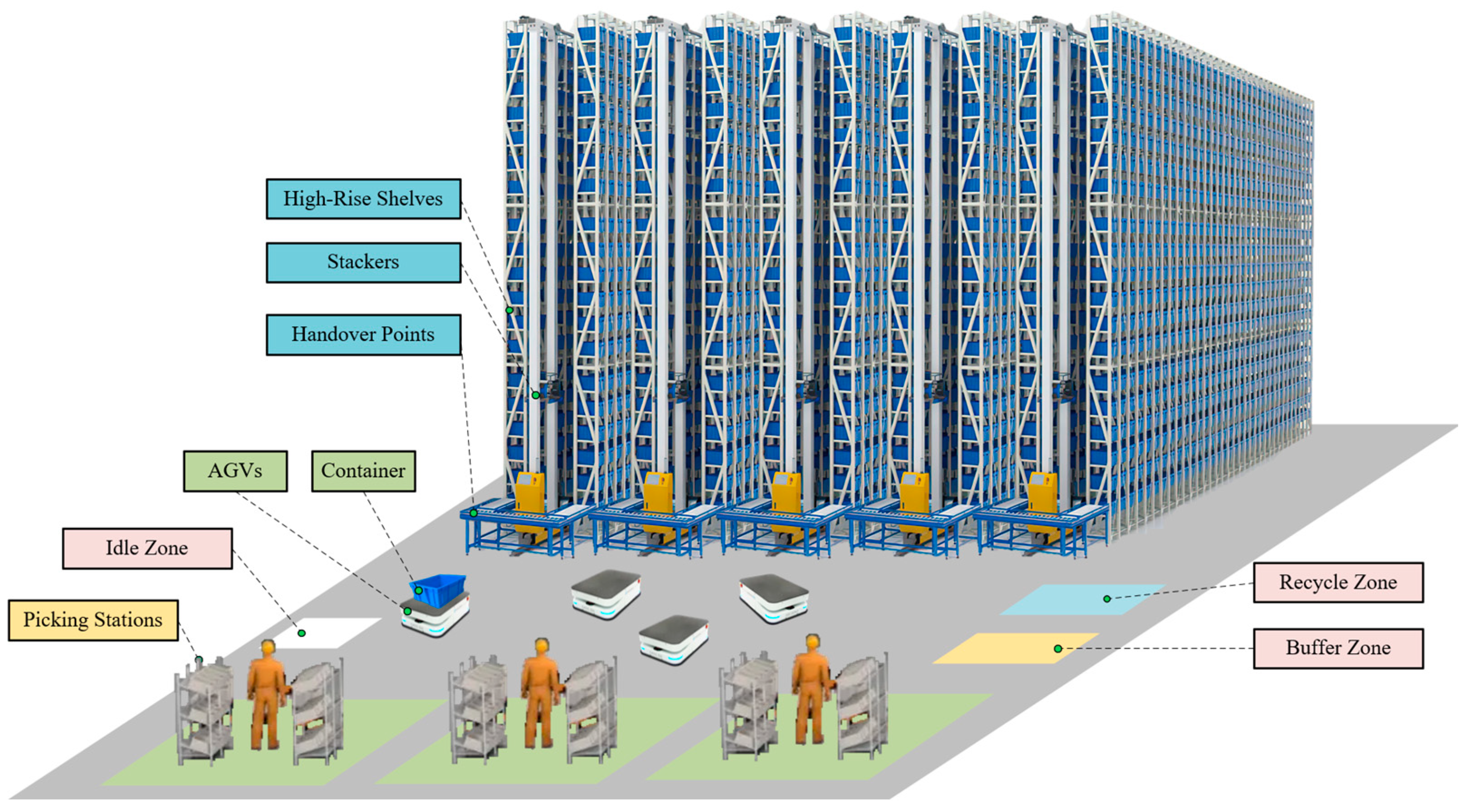
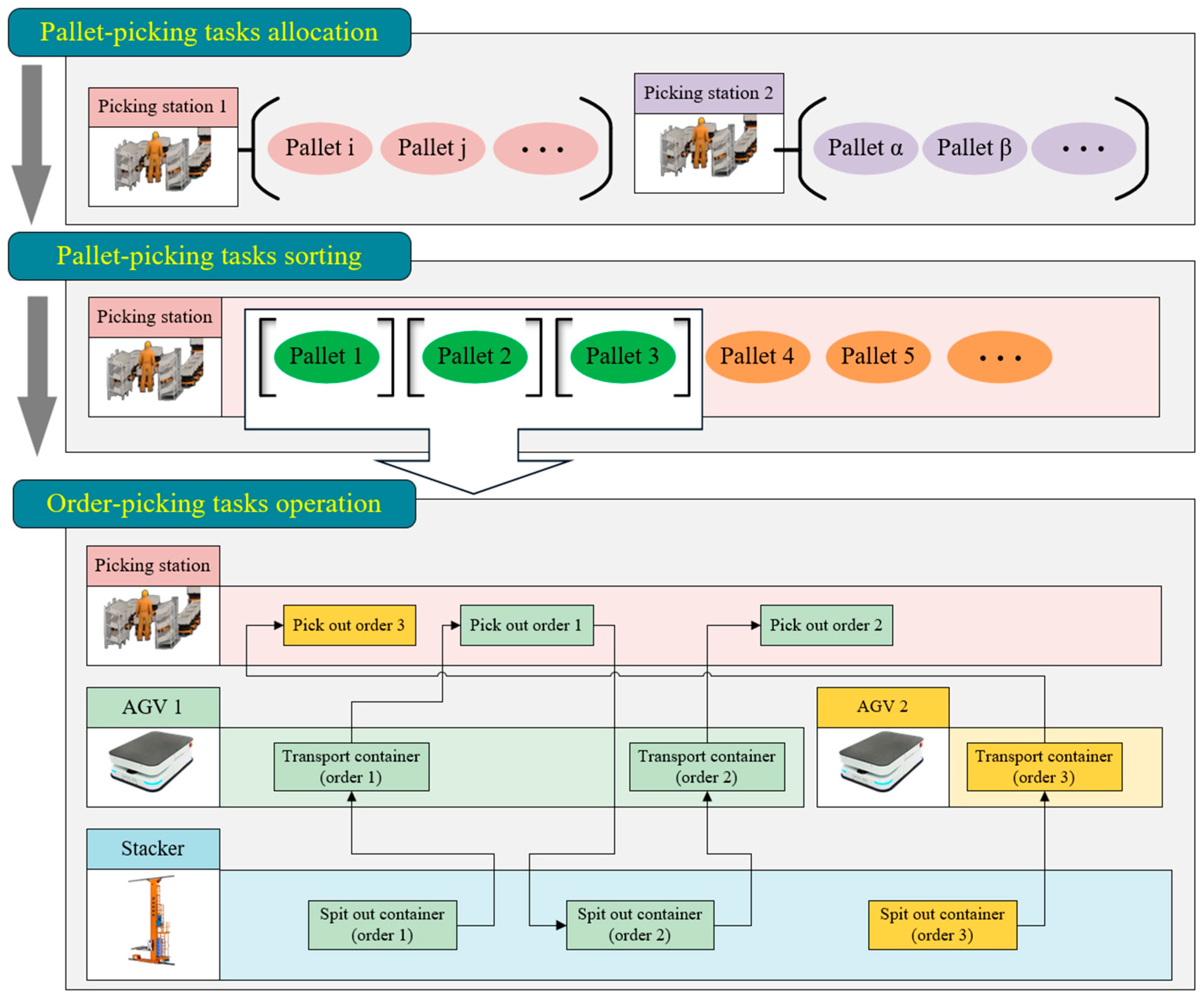
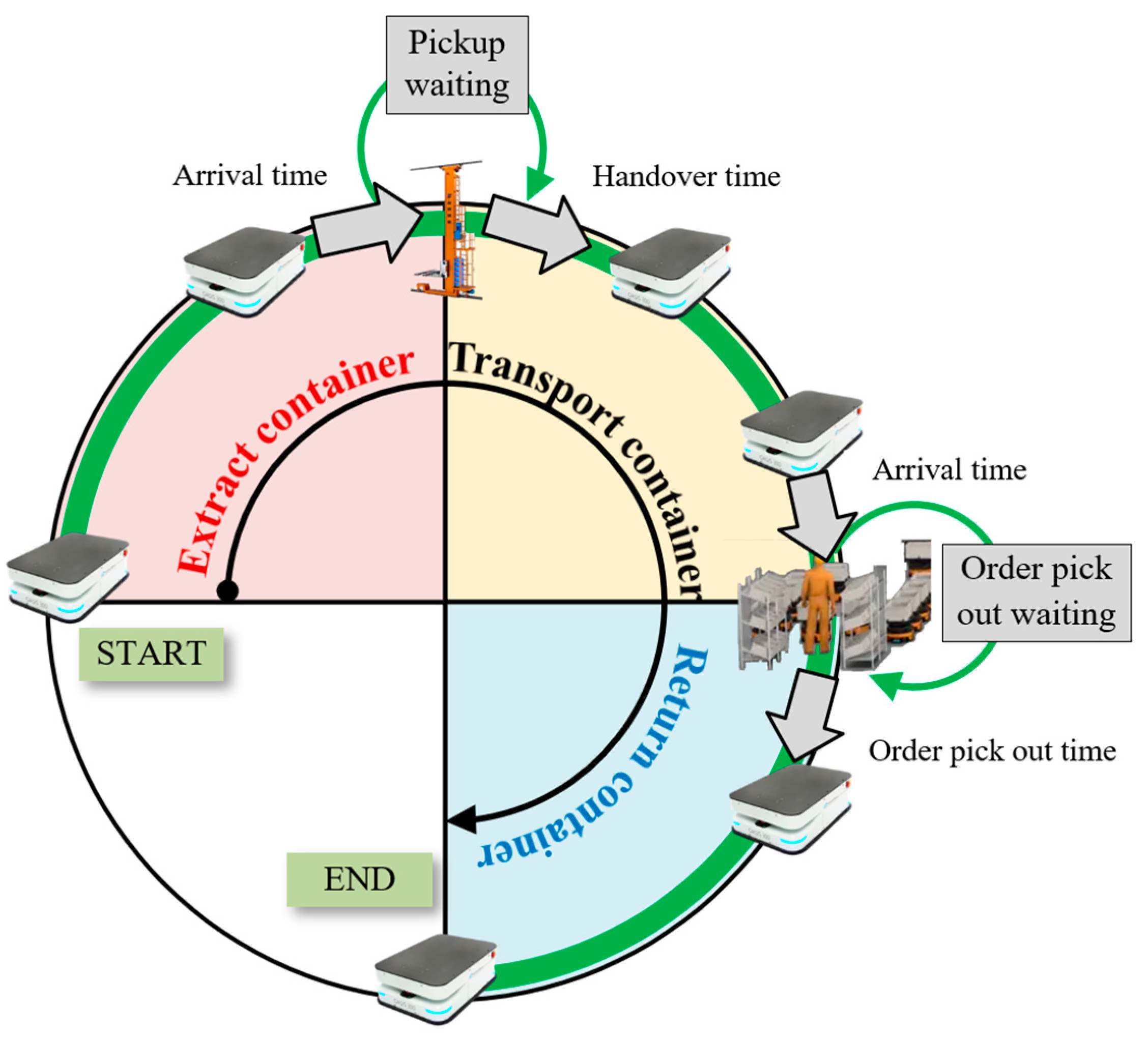
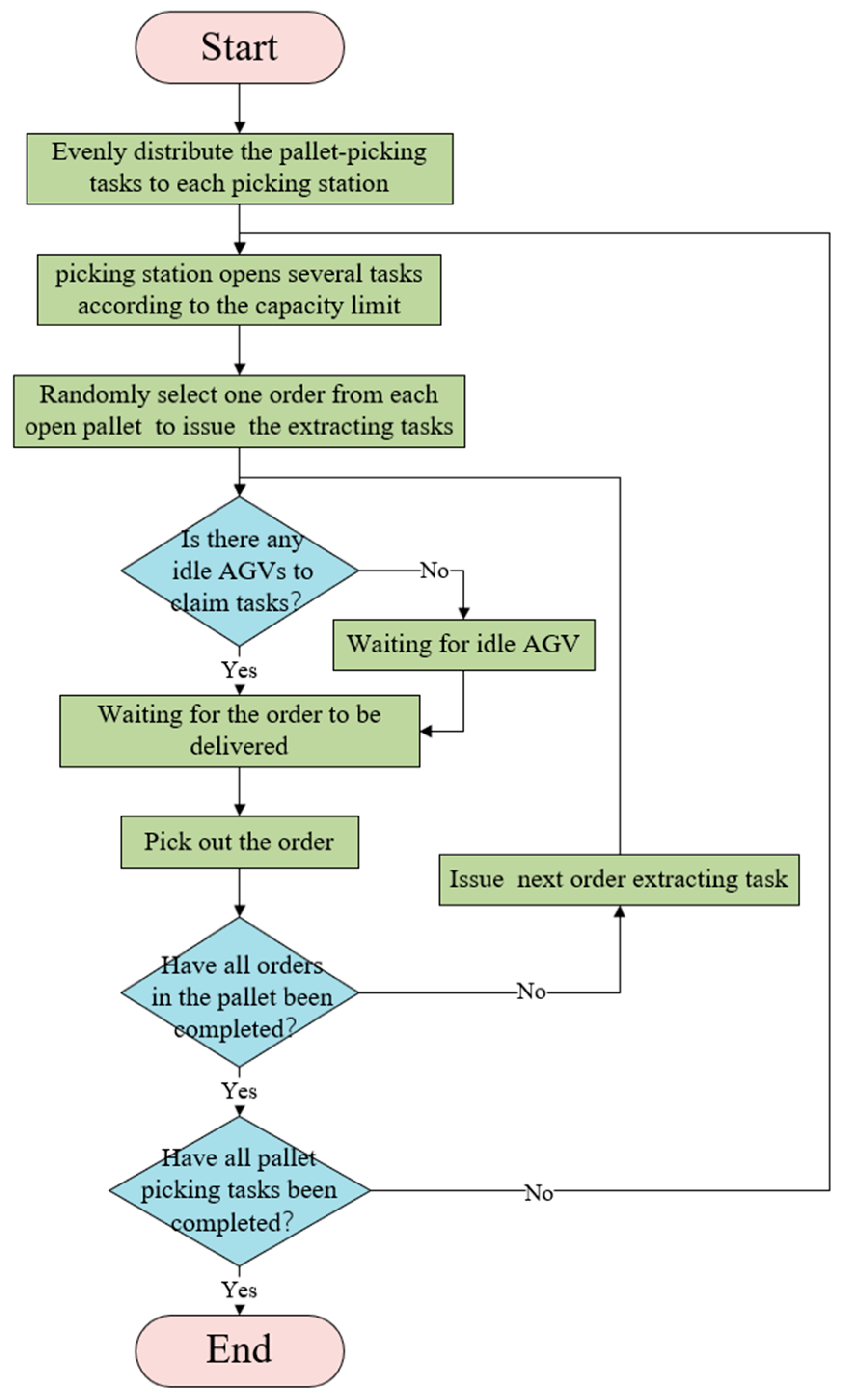


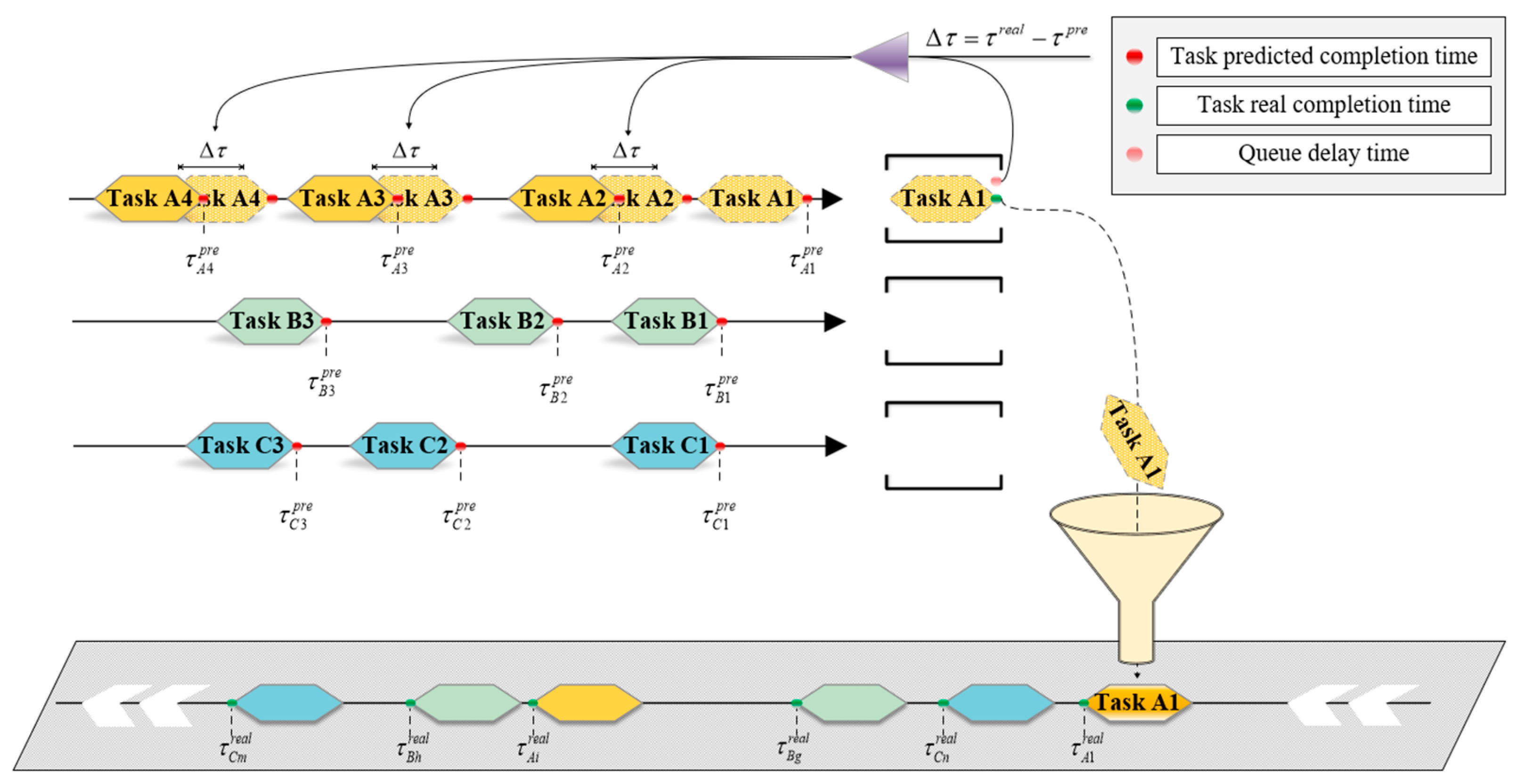
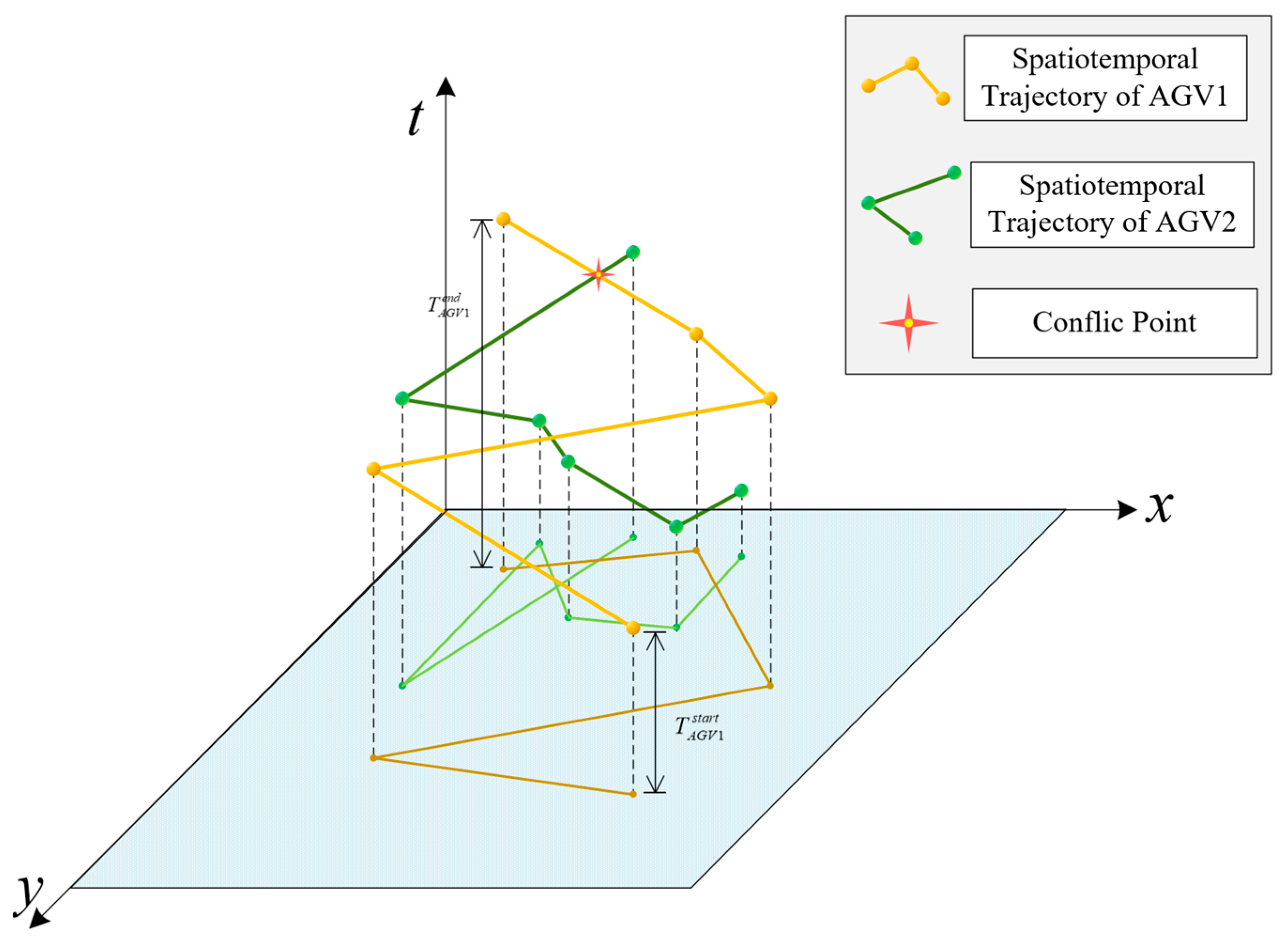
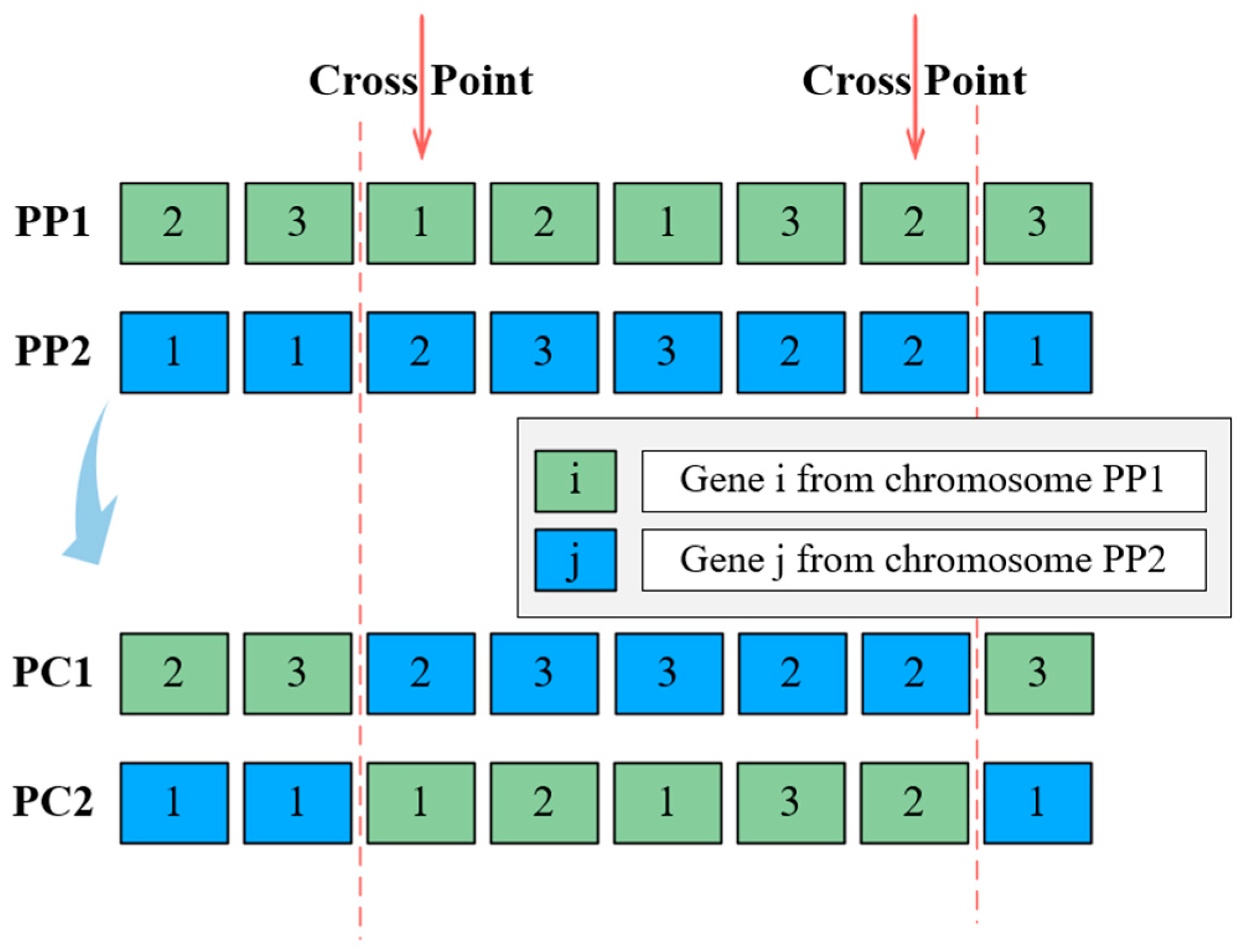

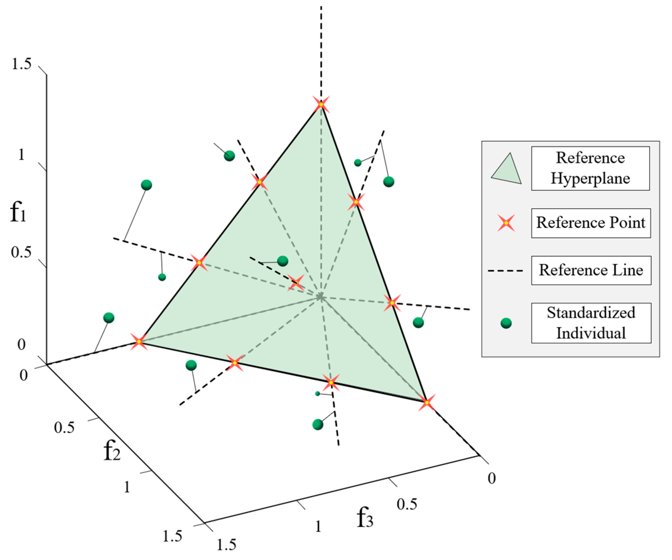
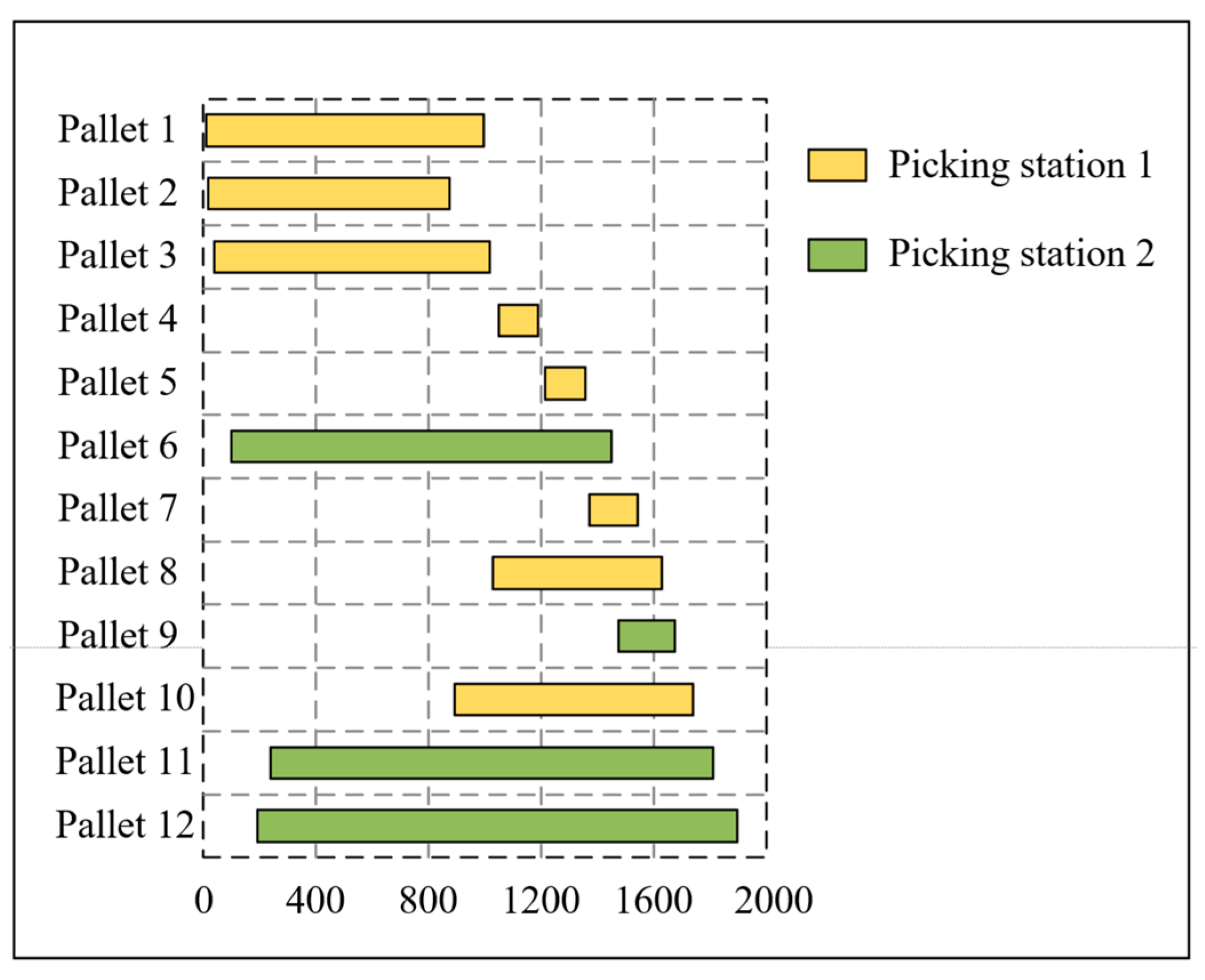
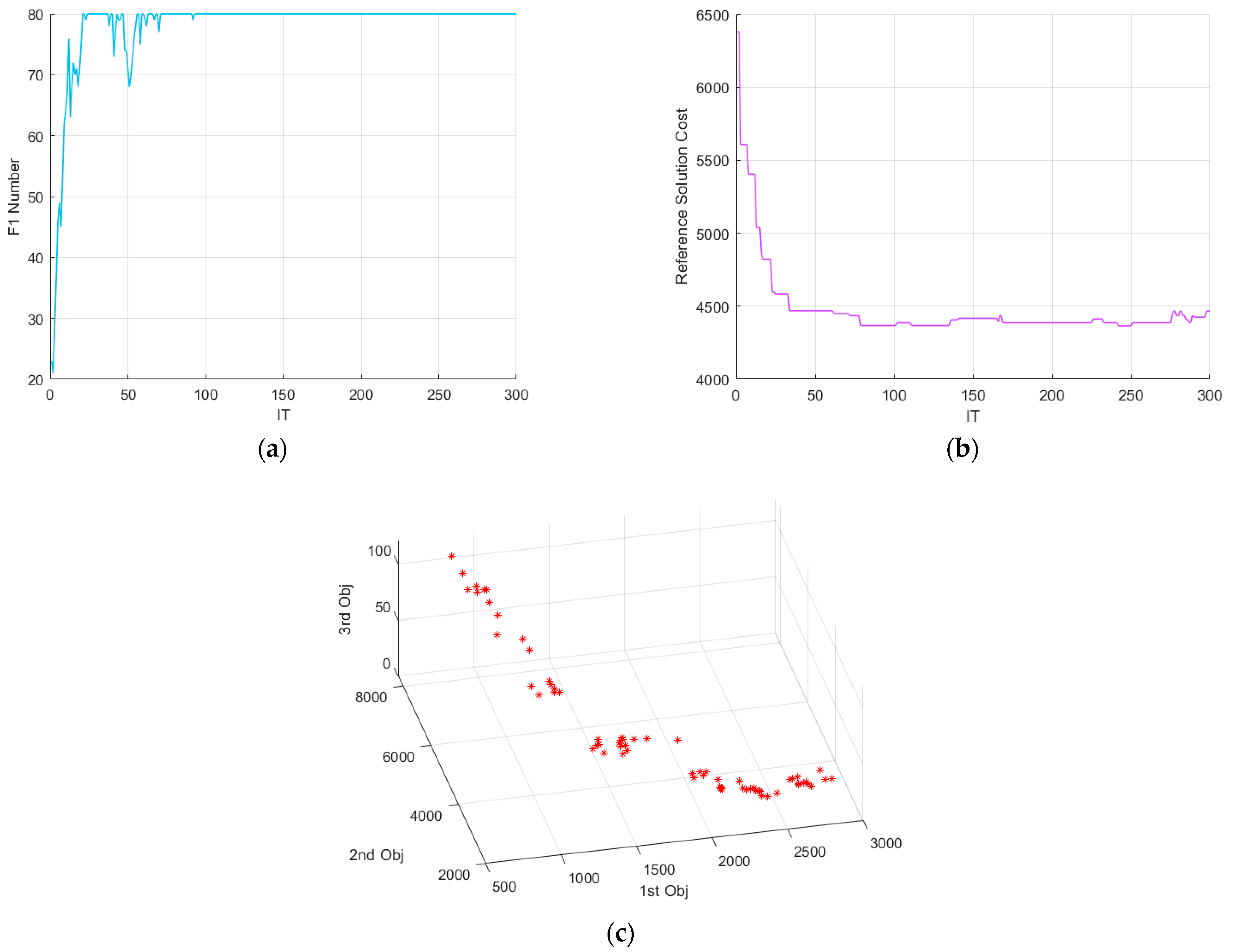
