Comparative Performance Analysis of Deep Learning, Classical, and Hybrid Time Series Models in Ecological Footprint Forecasting

Abstract

In a globalized world, factors such as increasing population, rising production rates, changing consumption habits, and continuous economic growth contribute significantly to climate change. Therefore, successfully forecasting the Ecological Footprint (EF) effectively indicates global sustainable development. Despite the significant role of the EF as one of the indicators of sustainable development, there is a gap in the literature regarding time series methods and forward-looking predictions. To address this gap, Ecological Footprint (EF) forecasting was performed using deep learning methods such as LSTMs, classical time series methods like ARIMA and Holt–Winters, and the developed hybrid ARIMA-SVR model. In the scope of the study, first, a spreadsheet was created using the total Ecological Footprint (EF) worldwide between 1961 and 2022, obtained from the Global Footprint Network database. Second, the forecasting performances of the ARIMA, Holt–Winters, LSTM, and the hybrid ARIMA-SVR models were compared using MAPE and RMSE metrics. Finally, the forecasting performances of the time series models were statistically validated through Wilcoxon Signed-Rank and Friedman tests. The study findings indicate that the proposed ARIMA (1,1,0) model demonstrated better performance with an average MAPE of 2.12%, compared to Holt–Winters (MAPE of 2.27%), LSTM (MAPE of 3.19%), and ARIMA-SVR (MAPE of 2.68%) methods in the test dataset. Additionally, it was observed that the ARIMA model forecasted the EF, which experienced a sudden decrease due to the COVID-19 lockdown, with a lower error compared to other models. These findings highlight the adaptability of the ARIMA model to variable and uncertain conditions.

1. Introduction

Worldwide rapid population growth, industrialization, and urbanization, along with increases in production and consumption, are exacerbating environmental issues. These problems have particularly impacted environmental and natural resource economists, especially in the areas of climate change and global warming. Complex relationships among economic growth, energy consumption, urbanization, natural resources, economic freedom, and Ecological Footprint create an interconnected and dynamic context. The Ecological Footprint assesses various human-induced activities such as agricultural land, seas and fishing areas, grazing lands, developed land, forest products, and carbon footprint [1]. This measurement, a quantitative indicator of sustainable development, particularly includes the consumption footprint (gha), which encompasses the area required to produce consumed materials and the area needed to absorb carbon dioxide emissions [2].

Ecological footprint and biocapacity are crucial concepts used to assess a region’s natural resource utilization and the services provided by ecosystems. While the Ecological Footprint measures how individuals, societies, or countries use natural resources, biocapacity determines how sustainably ecosystems can provide services [3]. In this context, biocapacity represents the capacity of nature to withstand human consumption. Countries that exceed their biocapacity, indicating a rapid depletion of natural resources and a significant increase in greenhouse gas emissions, are considered incapable of managing their resources sustainably [4]. This situation poses a serious threat to environmental sustainability.

Table 1. World total Ecological Footprint and biocapacity 2022 in gha/cap.

	Carbon	Crop Land	Grazing Land	Forest Products	Fishing Grounds	Built-Up Land	Total
Ecological Footprint	1.562	0.485	0.125	0.264	0.083	0.063	2.582
Biocapacity		0.485	0.184	0.643	0.136	0.063	1.510
Ecological Deficit							−1.072

includes the global Ecological Footprint and biocapacity data for the year 2022 [5]. These data are presented on a per capita basis in global hectares (gha/cap) and encompass components of carbon, crop land, grazing land, forest products, fishing grounds, and built-up land.

When Table 1 is examined, the average Ecological Footprint per capita was measured as 2.582 gha/cap in the year 2022. This value indicates that the per capita consumption globally surpasses the capacity allocated for the sustainability of ecosystems, exceeding ecological balance. This situation poses a significant concern for the long-term health of ecosystems and conservation efforts to maintain the balance of nature, as evidenced by instances such as the rapid decline of the Amazon rainforest and the excessive use of water resources.

Biocapacity was recorded as 1.510 gha/cap in the year 2022, representing the capacity of nature to withstand human consumption. Ecological Overshoot, on the other hand, indicates the situation where total consumption exceeds biocapacity, and was measured as −1.072 gha/cap in 2022, meaning that global consumption is below biocapacity. This negative value signifies that the sustainability of the utilized resources falls short, indicating that ecosystems cannot meet the demands of consumption.

According to the presented data in Table 1, a balance is observed in crop land and built-up areas, while it is observed that the biocapacity is exceeded in forest grounds and grazing lands. This situation indicates a tendency in sectors such as forestry and livestock to exceed natural resources, often driven by the need to meet increasing demands. The data in Table 1 emphasizes the importance of sustainability efforts and the effective management of natural resources. Increasing measures for ecosystem conservation and considering these data in policy development processes are crucial for a sustainable future.

Time-dependent predictions are widely utilized across various fields, serving as a critical tool for comprehending, assessing, and forecasting future events and trends. Especially through time series models, these predictions provide an effective method for forecasting future values based on past datasets. By thoroughly analyzing patterns and changes in previous periods, these models offer valuable insights into future trends. Despite the widespread use of time-dependent predictions in various fields, there is a literature gap concerning a standardized or comprehensive assessment that measures the applicability of time series models in predicting Ecological Footprint.

In this study, the forecasting of Ecological Footprint (EF) was performed using various time series models, and the performances of these models were compared. In this context, the deep learning model of Long Short-Term Memory (LSTM), classical time series methods such as Auto-Regressive Integrated Moving Average (ARIMA), and Holt–Winters, and a developed hybrid model combining ARIMA with Support Vector Regression (ARIMA-SVR) were used. The study findings demonstrated that the ARIMA model, known as a popular and successful method in the literature, outperformed other methods in EF forecasting.

The contributions of this paper can be summarized as follows:

• Evaluating the forecasting capabilities of LSTMs, ARIMAs, Holt–Winters, and hybrid ARIMA-SVR models for the worldwide Ecological Footprint (gha).
• The ARIMA (1,1,0) model is recommended for Ecological Footprint forecasting.
• Comparing the forecasting performances of models under unforeseen decrease conditions due to COVID-19 lockdowns.
• Statistically validating the performance of the proposed ARIMA (1,1,0) model.

2. Literature Review

In recent years, studies have been conducted using artificial intelligence to make predictions based on Ecological Footprint data.

Liu et al. [6] performed EF prediction for Beijing by utilizing a dataset comprising 10 different input variables from 1996 to 2015, including population, total foreign trade, and total energy consumption, with EF as the output variable. Tested the prediction performances of the BPNN and SVM models for 2014 and 2015. According to the results of the relative error rates, it has been reported that the SVM model made more successful predictions compared to the BPNN model. Consequently, the SVM model was employed for EF prediction for the years 2016–2020.

Yao et al. [7] calculated the EF value for the years 1999–2018 and simulated the EF value with ARIMA and Grey Model (GM). The models were evaluated according to the fitting performance criterion. Since the p value of the GM (1,1) model is lower in the fitting performance evaluation, the EF values for 2019 and 2024 are estimated with the GM (1,1) model.

Wang et al. [8] used ARIMA and the hybrid ARIMA-ANN models for estimating Ecological Footprint and ecological capacity in China. The Root Mean Square Error (RMSE) and the Mean Absolute Percentage Error (MAPE) metrics were used in comparing the model performances. The forecasting results of the study demonstrated that the hybrid ARIMA-ANN performed better than other models.

Xu [9] predicted the per capita ecological carrying capacity of Shenzhen, China using the ARIMA-LSTM hybrid method. Data from the years 2013 to 2018 were utilized in the study. Different learning rate values for the model were experimented with, and the optimal parameter (Learning rate 0.0005) was chosen for the best MAE and RMSE.

Jia et al. [10] utilized the ARIMA model for the estimation of the Ecological Footprint (EF) in Henan Province, China. In the study, EF and Ecological Carrying Capacity (EC) were initially calculated for the years 1949–2006. The calculated values were then used to evaluate the forecasting performance of the ARIMA model. The success of the ARIMA model was assessed based on fitting performance and was not compared with the success of a different method.

Roumiani et al. [11] calculated the Ecological Footprint of the top 10 countries with the best tourism destinations. Multiple regression and artificial neural network models were employed for this purpose. The study utilized information on natural resources, international tourists, economic growth, human capital, and Ecological Footprint between 1995 and 2019. Findings from the study indicated a significant positive correlation between economic growth and Ecological Footprint, with the ANN model demonstrating greater success. Therefore, the ANN model was reported to be more suitable for Ecological Footprint estimation in these countries.

Janković et al. [12] aimed to predict total EF consumption using information on population, oil, gas, coal, solar, other renewables, wind, nuclear, and hydro. For this purpose, K-Nearest Neighbors Regression (KNNReg), Random Forest Regression (RFR), Artificial Neural Network (ANN) with Rectified Linear Unit (ReLU), and ANN with Scaled Parametric Orthogonal Code Update (SPOCU) methods were employed. The performance of these methods was measured using MASE, NRMSE, MAPE, and SMAPE. The results indicated that the KNNReg model outperformed the others. Additionally, in the study, EF predictions are made using a GUI developed with the model that exhibited the best performance.

Moros-Ochoa et al. [13] conducted the prediction of Biocapacity and Ecological Footprint using a deep neural network. Different parameters of the DNN model were tested, and the performance of the models was measured using MAE and MSE metrics. With the DNN model exhibiting the lowest error, the footprint estimates for fishing grounds, grazing lands, forest lands, cropland, and built-up land worldwide for the years 2018–2030 were made.

When examining EF forecasting studies in the literature, it is observed that most research focuses on artificial intelligence prediction models to validate EF calculations. Only Moros-Ochoa et al. [13] have conducted forward-looking EF predictions using time series data and prediction models. However, in this study, EF predictions were made using only the NN model. Surprisingly, popular and successful models in the literature, such as ARIMA, Holt–Winters, and LSTM, were not utilized in EF prediction. This study aims to fill this gap in the literature and analyze the prediction capabilities of LSTM, ARIMA, Holt–Winters, and the hybrid ARIMA-SVR model to measure their EF forecasting abilities using different time series models

3. Materials and Methods

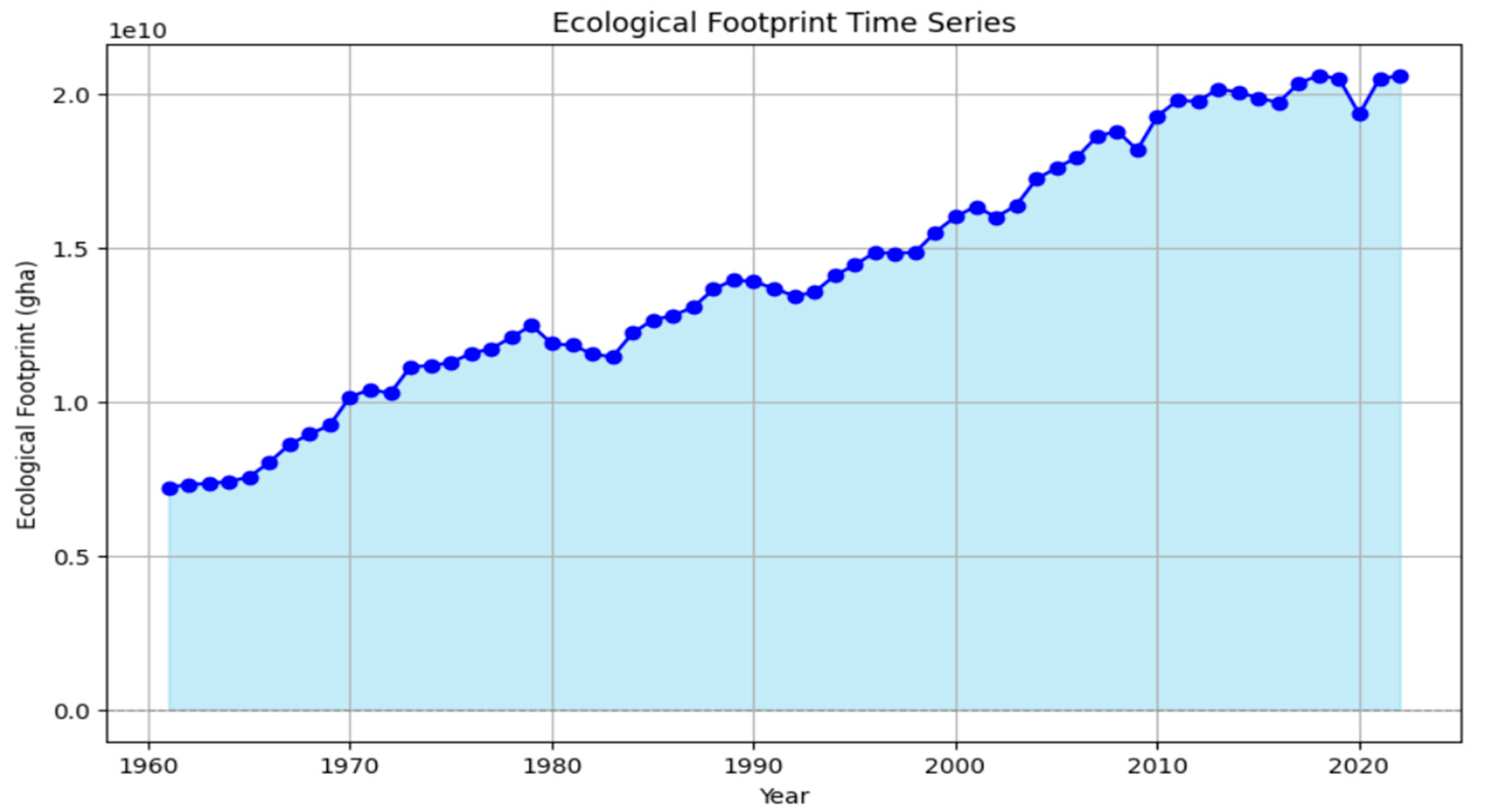
The dataset used in the study has been obtained from the Global Footprint Network database [14], encompassing the annual total Ecological Footprint amounts worldwide from 1961 to 2022. This time series is presented in Figure 1.

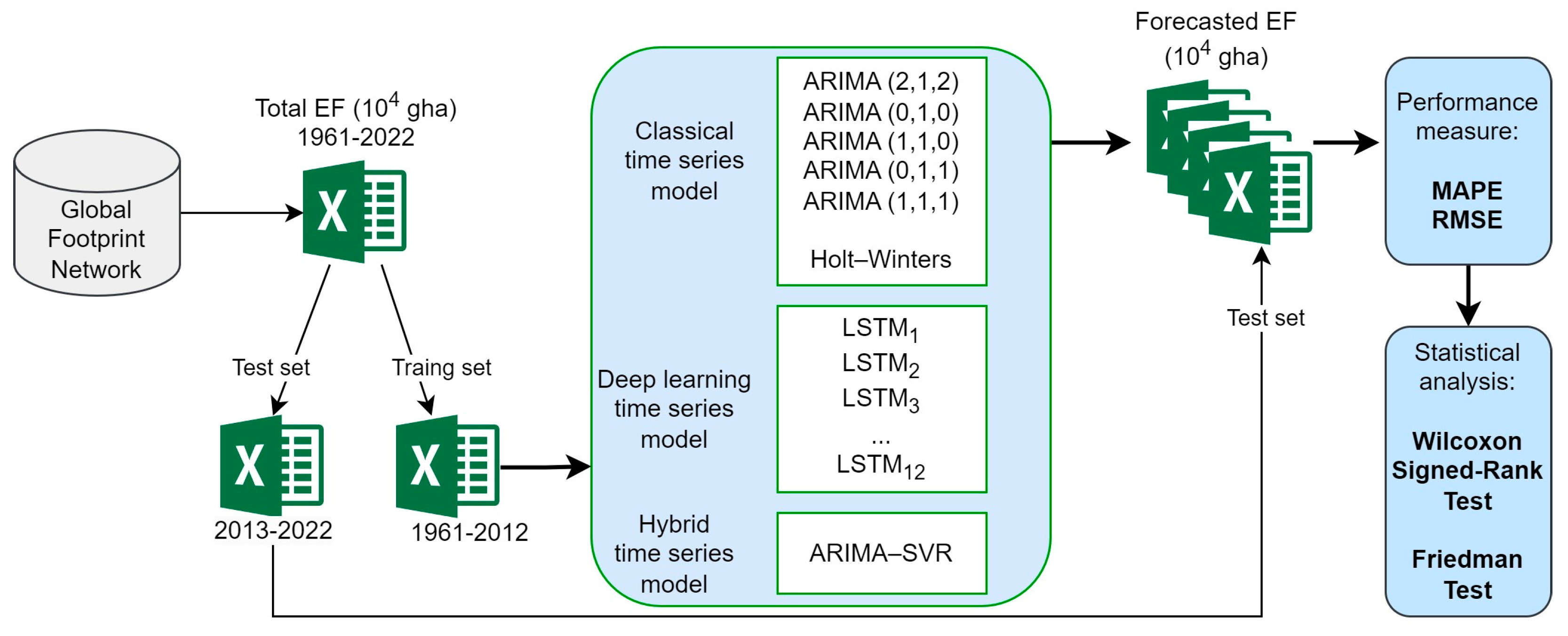
The framework of the study for EF forecasting is illustrated in Figure 2. Firstly, total EF (10⁴ gha) data by year were collected into an Excel file for worldwide Ecological Footprint forecasting. The dataset was divided, allocating 85% for training (1961–2012) and using the remaining 15% to evaluate the model performances. Subsequently, we trained five ARIMA models, Holt–Winters, twelve LSTM models, and the developed hybrid ARIMA-SVR model using the dataset from 1961–2012. EF forecasts were generated for each year until 2022, covering a span of 10 years. The forecasted values of the models were then compared with the test set, and MAPE and RMSE values were measured. In the final stage, we validated the predictive abilities of the models using the Wilcoxon Signed-Rank and Friedman Tests.

In this study, various time series models with different structures, including classical, deep learning, and hybrid models, were chosen to identify the model that best suits the data and exhibits effective predictive performance in forecasting the Ecological Footprint. The ARIMA model is an effective tool for addressing trend and seasonal components in time series, and it also fits well with linear data [9]. LSTM, an effective deep learning algorithm designed to capture long-term dependencies in time series, also demonstrates a robust predictive effect on nonlinear data [9]. The Holt–Winters model includes a triple exponential smoothing method that can handle irregular changes in time series [14]. In the hybrid ARIMA-SVR model, a more flexible model is developed by combining the predictive capabilities of ARIMA with the SVR’s ability to model nonlinear relationships.

The statistical analyses of this study and the developed LSTM, ARIMA, Holt–Winters, and hybrid ARIMA-SVR models were executed using the Python programming language. Python is a user-friendly programming language with a wide range of applications. The unique design of this high-level programming language allows for easy code reuse.

3.1. Ecological Footprint Dataset

The Ecological Footprint data used in this study was obtained from the Global Footprint Network website [15]. From this database, the global hectares (gha) amount of total Ecological Footprint (EF) from 1961 to 2022 was acquired. The database provides distinct quantities for 184 countries regarding crop land, forest land, grazing land, fishing grounds, built-up land, and carbon components, presented in global hectares (gha). 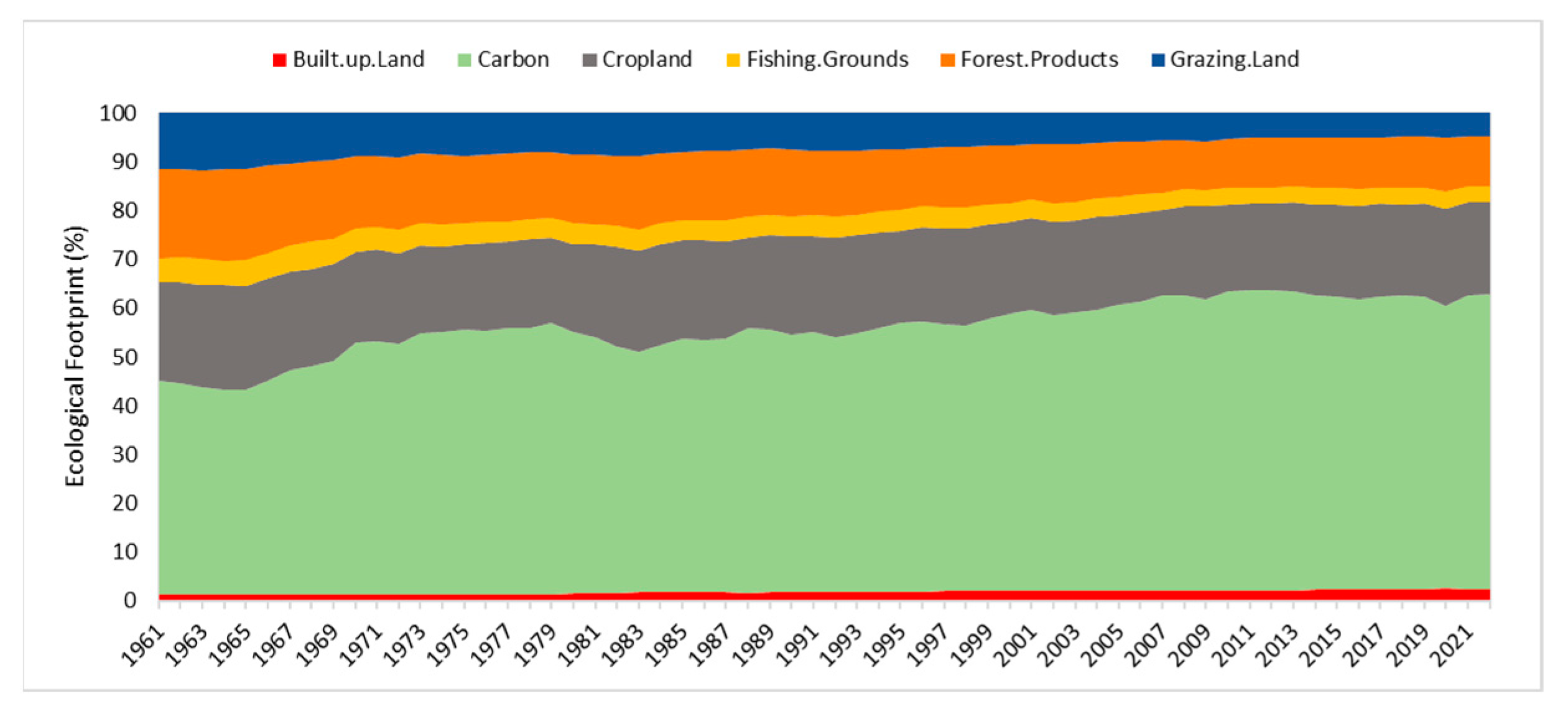Figure 3 illustrates the worldwide Ecological Footprint amount formed by the proportions of these components.

Figure 3 highlights significant results by illustrating the overall proportion of EF components worldwide. Between 1961 and 2022, the carbon footprint constitutes more than 50% of the total EF, emerging as a significant component of the Ecological Footprint. Cropland, the second-largest contributor, follows the carbon footprint, and these components together shape a substantial portion of the overall EF, defining the general outlook of the Ecological Footprint.

Additionally, it is observed that the built-up land component has a lower impact level compared to other components. This indicates that the contribution of construction and urban areas to the Ecological Footprint is lower than other components. Figure 3 improves the comprehension of environmental impacts by illustrating the relationships among the components of the Ecological Footprint from 1961 to 2022 and showcasing the sustainability performance of these components.

The general information regarding the features that constitute the EF components in the dataset is provided below [16]:

Carbon is one of the six footprint components present in the dataset used in the study. Constituting approximately 55.7% of the total Ecological Footprint, it measures CO₂ emissions resulting from fossil fuel usage. The carbon footprint reached its highest value in the year 2022 (12.456 billion gha), and upon examining 62 years of data (1961–2022), the average carbon footprint is observed to be 7.957 billion gha (global hectares). The continual increase in carbon footprint each year, reaching 12.456 billion gha in 2022, signals a concerning development in terms of environmental sustainability. Currently, the carbon footprint constitutes the most significant portion of humanity’s overall Ecological Footprint. These elevated values reflect the rising use of fossil fuels and associated CO₂ emissions [17]. The intensive use of fossil fuels can worsen problems like global warming, climate change, and environmental imbalance [18].

Crop Land comprises approximately 19% of the total worldwide EF between 1961 and 2022. The average cropland footprint over 62 years is approximately 2.72 billion gha. Crop Land, representing agricultural land, significantly influences the determination of the carbon footprint and contributes to carbon emissions. This agricultural land supports food production for human consumption, animal feed, oilseeds, and other agricultural products [19]. Soil cultivation, alteration of vegetation cover, and agricultural practices result in the release of carbon into the atmosphere [20]. Therefore, cropland is a component considered in carbon footprint calculations and emphasizes the importance of sustainable agricultural practices. The management of this area focuses on reducing carbon emissions and enhancing soil carbon, contributing to environmental sustainability.

Grazing Land is an area used for raising animals for meat, milk, leather, and wool products. The Ecological Footprint of this category is calculated by comparing the amount of animal feed in a country to the total feed required for all animals in that year. It is assumed that the remaining demand for animal feed comes from grazing land [21,22]. When examining the grazing land component in the dataset used in the study, it is observed that it experienced a decline after 1995, reaching approximately 998 million gha in 2022, with a 62-year average of 991 million gha. Additionally, as depicted in Table 1, the biocapacity in grazing lands has been exceeded. Therefore, it is crucial to implement strategies that prevent the excessive use of biocapacity in grazing lands and promote sustainable usage practices.

The Forest Product footprint is calculated based on a country’s annual consumption of timber, pulp, timber products, and fuelwood [23]. It also includes carbon dioxide emissions resulting from the burning of fossil fuels. In this context, it accounts for the embedded carbon in imported products. The Forest Product Footprint represents the forest area required to absorb these carbon emissions. As a component within the Ecological Footprint, the Forest Product Footprint is crucial for assessing the sustainable management of forest resources and understanding the carbon balance. This metric measures the net impact of human interactions on forest ecosystems and is a significant component of the contemporary Human Footprint [16].

Built-up Land is a metric calculated based on the total land area covered by human infrastructure, including elements such as transportation, housing, industrial structures, and reservoirs used for hydroelectric power [16]. It may also encompass areas previously used for agriculture, making this metric important for assessing how human interactions have altered natural ecosystems and transformed the prior functions of the utilized land. The Built-up Land Footprint is employed to understand the environmental impacts of urban development and infrastructure projects, providing guidance for sustainable planning efforts [24].

3.2. Autoregressive Integrated Moving Average (ARIMA) Model

ARIMA is a popular and successful classical statistical time series forecasting method based on past data [14,25,26]. This model is designed to capture trends, cycles, and fluctuations based on observations over time [27]. It is typically expressed as ARIMA(p, d, q), where p, d, and q denote the orders of autoregressive (AR), difference (I), and moving average (MA) components, respectively. The time series in the ARIMA model should be stationary. If the time series is not stationary, a differencing operation is applied, and d indicates the number of times this differencing operation is performed. The Augmented Dickey–Fuller (ADF) test is used to assess the stationarity of the time series. The ADF test determines the presence of a unit root in a time series, checking whether the series is stationary. If a time series is not stationary, the differencing operation is continued to make the series stationary, allowing the ARIMA model to be applied more effectively.

In the Box–Jenkins approach, four steps are followed to model the ARIMA process. In the first step, the model is identified; in the second step, parameter estimation and selection are performed; in the third step, model verification is conducted; and finally, in the fourth step, predictions are made.

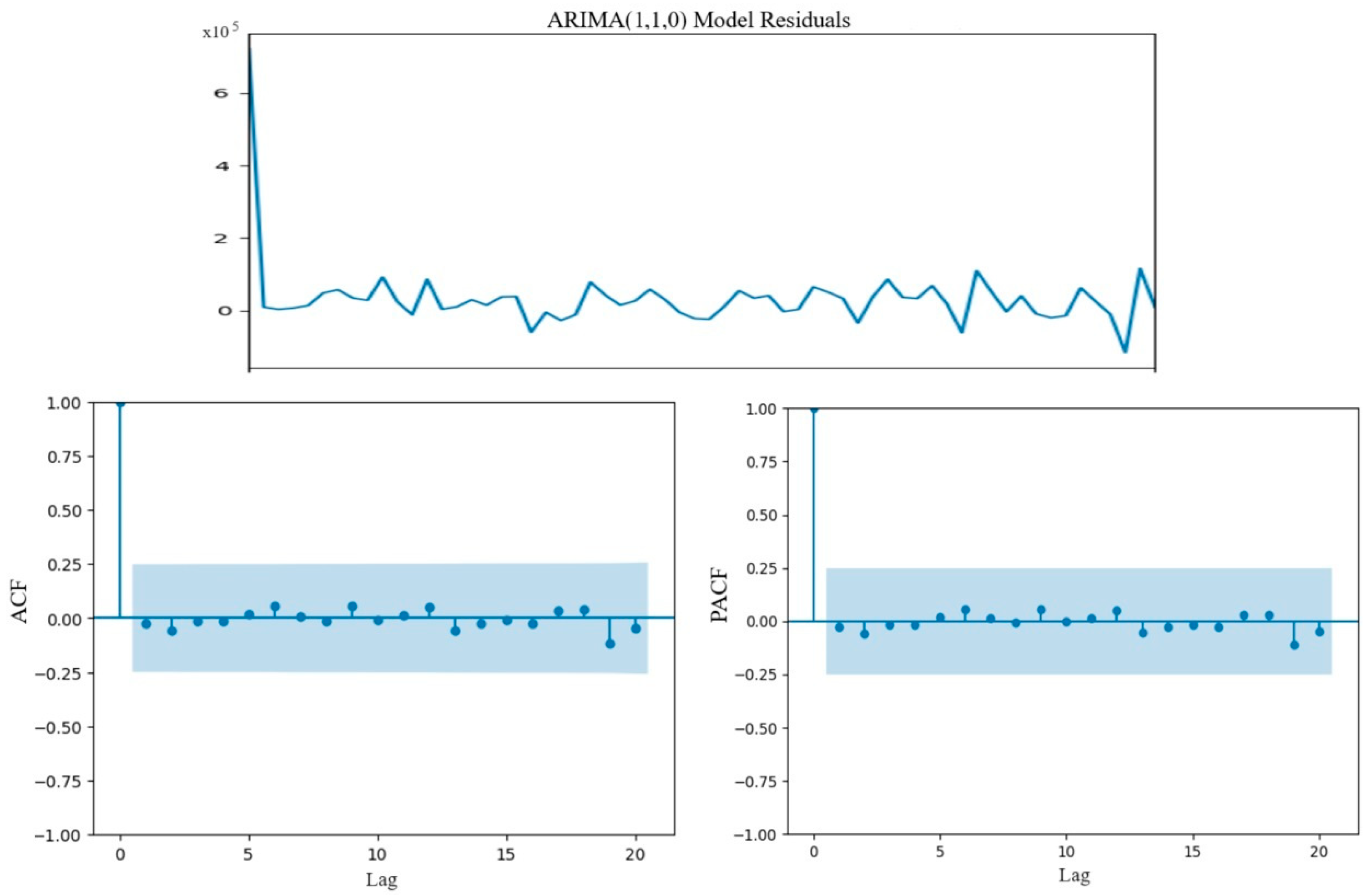
The autocorrelation function (ACF) and partial autocorrelation function (PACF) plots are used to determine the q and p values of the ARIMA model. However, it may not always be possible to make accurate observations on the graph. Therefore, the most suitable ARIMA model can also be determined using Akaike Information Criterion (AIC), Bayesian Information Criterion (BIC), and Corrected Akaike Information Criterion (AICc) values. Additionally, strictly adhering to AIC, BIC, and AICc criteria may not always yield accurate results. Therefore, to determine the most suitable model for the dataset, it is recommended to assess ARIMA models on the test set.

The formulas for AIC, BIC, and AICs statistical metrics are given in Equations (1)–(3), respectively.

$$AIC=-2\log \left(ML\right)+2k$$

(1)

$$BIC=-2\log \left(ML\right)+klog\left(n\right)$$

(2)

$$AICc=-2\log \left(ML\right)+2k+\frac{2k(k+1)}{n-k-1}$$

(3)

Here, k represents the count of estimated parameters within a specific model, n denotes the size of the sample, and log(ML) stands for the maximized log-likelihood function tailored for the suggested model.

3.3. Long Short-Term Memory (LSTM) Model

Long Short-Term Memory (LSTM) is a recurrent neural network architecture designed specifically for working with time series and sequential data [28]. The fundamental feature of LSTM is its ability to learn long-term dependencies, allowing it to understand and utilize long-term dependencies without losing short-term memory capabilities. The basic structure of the LSTM architecture is provided in Figure 4.

The Hidden State (H_t) and Cell State Update (C_t) indicate how the LSTM model progresses from one-time step to the next and updates the information it contains. These two components enhance the model’s learning and information retention capabilities by updating the hidden state, representing the network’s previous state, and the memory cell. While H_t typically represents the outputs presented by the model to the external world, C_t signifies the internal memory state of the model. These two states empower the LSTM to learn long-term dependencies.

The hidden state update involves the following steps:

Output Gate (O_t): This utilizes a sigmoid activation function to determine the amount of information to extract from the cell state. This controls if more or less information is extracted from the cell state. The O_t value is a number between 0 and 1.

Cell State (C_t): This represents the updated cell state from the LSTM’s memory unit.

Hidden State Update (H_t): This is updated using the formula in Equation (4).

$${\mathrm{H}}_{\mathrm{t}}={\mathrm{O}}_{\mathrm{t}}\tanh \left({\mathrm{C}}_{\mathrm{t}}\right)$$

(4)

In this formula, the hyperbolic tangent (tanh) activation function compresses the cell state value into the range [−1, 1]. Afterward, the result is multiplied by the ratio determined by the output gate. This process determines how the information learned by the LSTM will be reflected in the vector representing the hidden state.

The Cell State Update (C_t) involves the following steps:

Forget Gate (f_t): A sigmoid activation function is used to determine which information from the previous cell state will be forgotten. Values approaching 0 imply complete forgetting, while values approaching 1 indicate complete remembrance.

Input Gate (I_t): A sigmoid activation function is used to determine how much of the new information will be added to the cell state. Values approaching 0 imply ignoring the new information, while values approaching 1 indicate fully incorporating the new information.

Candidate Memory ($\widetilde{{\mathrm{C}}_{\mathrm{t}}}$): This represents the candidate cell state, which represents the new information. It is processed using the tanh activation function and compressed into values between -1 and 1.

Cell State Update (C_t): It represents the result obtained by subtracting the forgotten part from the previous cell state using the forget gate and adding the new information using the input gate. Mathematically, it is expressed as in Equation (5).

$${\mathrm{C}}_{\mathrm{t}}={\mathrm{f}}_{\mathrm{t}}{\mathrm{C}}_{\mathrm{t}-1}+{\mathrm{I}}_{\mathrm{t}}{\tilde{\mathrm{C}}}_{\mathrm{t}}$$

(5)

3.4. Hybrid ARIMA-SVR Model

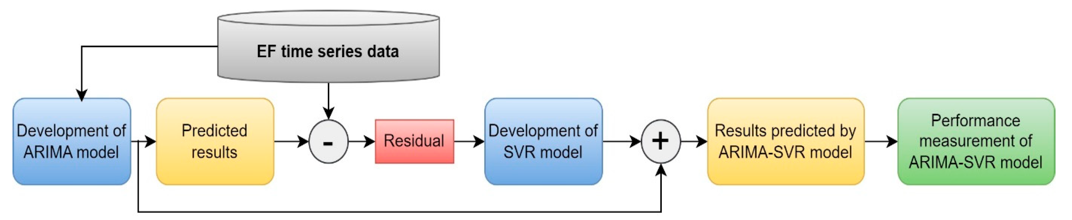
In this study, a hybrid ARIMA-SVR model was developed by combining the traditional Autoregressive Integrated Moving Average (ARIMA) and Support Vector Regression (SVR) methods. ARIMA is utilized to model the intrinsic dynamics of time series data and conduct regression analysis on corrected data, while SVR is integrated to address the model’s complexity and nonlinear features. This hybrid model aims to enhance the performance of time series forecasting by amalgamating the regulatory capabilities of ARIMA with the flexible learning capabilities of SVR. The flowchart of the ARIMA-SVR model is presented in Figure 5.

To determine the hyperparameters of the developed hybrid ARIMA-SVR model, a tuning process for support vector regression (SVR) was conducted using the Grid Search method. A dictionary named ‘param_grid’ was created to define the parameter range, encompassing options for determining the kernel type of the SVR model (‘linear’, ‘poly’, ‘rbf’, and ‘sigmoid’), values for the cost parameter (‘C’) (0.1, 1, 10, 100, 1000), and values for the epsilon parameter (‘epsilon’) (0.1, 0.2, 0.5, 0.3) to establish various parameter combinations. The Grid Search method was employed to execute trial and evaluation processes among these parameter combinations, identifying the ones with the best performance to obtain the optimal configuration for the model. Subsequently, the best parameters determined by the Grid Search method were utilized in creating the ARIMA-SVR model. The optimized parameters for the SVR model are as follows: ‘kernel’ is ‘linear’, ‘C’ is 1000, and ‘epsilon’ is 0.5. These parameters were selected to enhance the predictive ability of the ARIMA-SVR model for Ecological Footprint time series data.

3.5. Holt–Winters Model

Holt–Winters is a classic time series method commonly used for short-term forecasting [14]. Developed to predict future values of variables in time series that include both trend and seasonal effects, this method has a structure designed for such predictions. The approach employs three smoothing parameters to forecast the average level (L_t), slope (T_t), and seasonal component (S_t) of the time series [29]. These components are calculated as shown in Equations (6)–(8), and forecasting is performed using them, as indicated in Equation (9).

$$L_t=\propto \left(y_t-S_{t-s}\right)+\left(1-\propto \right)\left(L_{t-1}-T_{t-1}\right)$$

(6)

$$T_t=\beta \left(L_t-L_{t-1}\right)+(1-\beta ){ T}_{t-1}$$

(7)

$$S_t=\mathsf{\gamma }\left(y_t-L_t\right)+(1-\mathsf{\gamma })S_{t-s}$$

(8)

$$F_{t+k}=L_t+{kT}_t+S_{t+k-s}$$

(9)

Here, α, β, and γ are the smoothing parameters for the level, trend, and seasonal components, respectively.

3.6. Performance Evaluation Metrics and Statistical Tests

In this study, we assessed the performance of the models using the RMSE and MAPE metrics. RMSE represents the standard deviation of prediction errors, measuring the magnitude of differences between predicted and actual values. MAPE provides the average magnitude of prediction errors in percentage terms. Low RMSE and MAPE values indicate better model performance. The formulas for these metrics are given in Equations (10) and (11).

$$RMSE=\sqrt{\frac{1}{n}{\sum }_{i=1}^n{\left(x_i-y_i\right)}^2}$$

(10)

$$MAPE=\frac{1}{n}{\sum }_{i=1}^n\left|\frac{x_i-y_i}{x_i}\right|\times 100$$

(11)

Here, n represents the total number of observations, x_i denotes the actual value, and y_i represents the predicted value of the model.

In addition to these measures, the study employed the Wilcoxon Signed-Rank Test [30] and the Friedman Hypothesis Test [22] to compare the performance of prediction models. The Friedman Test was used to identify significant differences among multiple models, and the Wilcoxon Signed-Rank Test was employed to evaluate accuracy differences through pairwise comparisons of prediction models.

4. Results

The dataset used in this study has been divided into two parts: training and testing. Data from the years 1961 to 2012 (85% of the dataset) were used for training, while data from the years 2013 to 2022 (the remaining 15% of the dataset) were utilized to test the forecast performance of the models. During these forecasts, RMSE and MAPE values were employed to assess the accuracy of each model’s forecasts.

Comparison of Time Series Forecasting Models

Classical time series-based ARIMA and Holt–Winters models, the deep learning-based LSTM model, and our developed hybrid ARIMA-SVR time series prediction models were used to assess the predictability of the Ecological Footprint worldwide. The ADF test was performed to assess the stationarity of the time series, and the results are presented in

Table 2. ADF unit root test and difference results.

Data	ADF Test	Critical Value			p-Value	Stationarity
		1%	5%	10%
Original	−0.787	−3.542	−2.910	−2.593	0.823	Non-Stationary
First differenced	−6.703	−3.546	−2.912	−2.594	0.000	Stationary

. The ADF test statistic for the original series was calculated as −0.787, and the critical values for the significance levels of 1%, 5%, and 10% were −3.542, −2.910, and −2.593, respectively. Additionally, the calculated p-value (0.823), being higher than the significance alpha level (α = 0.05), indicates that the series is non-stationary. Therefore, to make the time series stationary, the first difference was taken (d = 1), and the ADF test was performed again. The calculated p-value for the first-differenced series is 0.000, indicating that it is stationary since this value is less than the 0.05 significance level, implying the absence of a unit root. With the series made stationary, the parameters of the ARIMA model can be determined.

To determine ARIMA model parameters, two approaches can be employed. Parameters are determined by examining Autoregressive Function (ACF) and Partial Autoregressive Function (PACF) plots [31]. Nevertheless, it may not always be feasible to observe the model’s structure through these plots. Therefore, model parameters can also be determined using automatic model selection. In Python programming, the ‘auto_arima’ function can be used to identify the most successful model. This function defaults to the AIC metric, but model selection can also be carries out based on BIC or AICc metrics. However, criteria like AIC, while generally helpful in model selection, may not always yield accurate results when strictly adhered to. Therefore, different ARIMA models were tested on the test set for Ecological Footprint predictions, and their performances were compared (

Table 3. Comparison of different ARIMA models on the test set.

Model	AIC	BIC	AICc	RMSE (104 gha)	MAPE (%)
ARIMA(2,1,2)	1336	1347	1337	59,696	2.27
ARIMA(0,1,0)	1345	1346	1345	59,696	2.27
ARIMA (1,1,0)	1349	1350	1346	59,536	2.12
ARIMA(0,1,1)	1345	1350	1346	59,609	2.16
ARIMA(1,1,1)	1347	1350	1345	60,398	2.27

). Using the same method, the 10-year data of the test set was predicted individually, and the metrics in the table were calculated. Subsequently, the averages of AIC, BIC, AICc, RMSE, and MAPE values for this 10-year test set were calculated and compared in Table 3.

The auto_arima function determines the best model based on AIC, BIC, and AICc metrics. The model selected by auto_arima, which has the lowest values for these metrics highlighted in bold in Table 3, is ARIMA(0,1,0). However, when different ARIMA models are tested on the EF dataset, it is revealed that the ARIMA (1,1,0) model has lower RMSE and MAPE values (Table 3, underlined bold). Therefore, the parameters p, d, q for the ARIMA model have been chosen as 1, 1, 0, respectively.

The suitability of the ARIMA (1,1,0) model was assessed utilizing the Ljung–Box test and ACF with PACF graphs. The Ljung–Box test, which relies on the sum of the squares of autocorrelation coefficients, is a statistical test that examines the significance of autocorrelation in the residuals of a time series. This test attempts to determine whether autocorrelation at a specific lag level exceeds a level of randomness. The ACF and PACF residual graphs shown in Figure 6 indicate the absence of significant autocorrelation, as the error correlations fall within the estimated threshold boundaries at various lags.

The results of the Ljung–Box test for the ARIMA (1,1,0) model are provided in

Table 4. Results of the Ljung–Box test for the ARIMA (1,1,0) model.

Model	Q	p-Value
ARIMA (1,1,0)	0.25	0.62

. If the p-value is greater than 0.05, the hypothesis is not rejected, indicating that autocorrelations are not statistically significant in this case. Since the p-value in the test result is greater than 0.05, it has been demonstrated that the ARIMA (1,1,0) model is suitable for Ecological Footprint time series data.

After identifying the ARIMA (1,1,0) model that best fits the dataset, the objective is to determine the LSTM model that is most suitable for the dataset. LSTM models possess the capability to capture more complex patterns and nonlinear relationships in time series data [32]. However, due to their numerous parameters, LSTM models can exhibit variable performance. Therefore, a series of trial and validation processes are necessary to identify an appropriate LSTM model. This process involves evaluating different configurations of LSTM models and selecting the one that achieves the best performance.

Different combinations of parameters were used to create a series of LSTM models, and these models were then trained with the dataset from 1961 to 2012, predicting values for the years 2013−2022. During the training of the LSTM model, the Mean Squared Error (MSE) performance metric was utilized for loss evaluation. The Rectified Linear Unit (ReLU), the most widely utilized activation function in deep neural networks, was utilized [33]. The Adam optimizer with a learning rate of 0.001 was chosen LSTM models were trained with randomly selected batch sizes, epochs, neurons, and dropout rate values. The trained models were used to forecast the Ecological Footprint for the last 10 years, and their performance was evaluated. The parameters and test set results of the LSTM models, including RMSE and MAPE, are presented in

Table 5. The RMSE and MAPE results of LSTM models with different hyperparameters.

Model	Batch Size	Epoch	Neuron	Dropout Rate	RMSE (104 gha)	MAPE (%)
LSTM1	1	100	50	0.4	503,752	24.95
LSTM2	4	50	50	0.2	322,527	15.96
LSTM3	4	150	150	0.4	518,833	25.70
LSTM4	8	50	128	0.0	118,784	5.85
LSTM5	8	250	128	0.2	236,088	11.67
LSTM6	16	200	128	0.0	97,094	4.85
LSTM7	16	150	100	0.2	322,728	15.97
LSTM8	16	200	100	0.4	484,008	23.97
LSTM9	32	100	100	0.2	373,708	18.50
LSTM10	32	150	150	0.4	495,785	24.55
LSTM11	32	150	150	0.0	139,483	6.88
LSTM12	32	250	128	0.0	64,030	3.19

. According to the test results, the LSTM₁₂ model, with parameters batch size = 32, epoch = 250, neuron = 128, dropout rate = 0.0, demonstrated the most successful outcome, yielding a 3.19% error and 64,030 × 10⁴ gha.

Finally, the hybrid ARIMA-SVR model was developed to forecast the Ecological Footprint. In developing the ARIMA-SVR model, the Grid Search method was employed to determine hyperparameters for support vector regression (SVR). Through various trials with Grid Search, the values C = 1000, epsilon = 0.5, and the ‘linear’ kernel function were determined for SVR.

The performances of the four different time series prediction models used in the study were compared based on the RMSE and MAPE metrics. In

Table 6. Comparison of EF forecasting performance of ARIMA, Holt–Winters, LSTM, and ARIMA-SVR models.

Year	ARIMA (1,1,0)		Holt–Winters		LSTM		ARIMA-SVR
	RMSE (104 gha)	MAPE (%)	RMSE (104 gha)	MAPE (%)	RMSE (104 gha)	MAPE (%)	RMSE (104 gha)	MAPE (%)
2013	40,469	2.01	5543	0.28	62,957	3.12	5914	0.29
2014	12,101	0.60	14,471	0.72	59,126	2.95	50,301	2.51
2015	19,299	0.97	51,732	2.61	52,831	2.66	54,677	2.75
2016	12,967	0.66	11,266	0.57	49,434	2.51	48,088	2.44
2017	63,556	3.12	54,274	2.67	54,053	2.66	29,533	1.45
2018	21,322	1.04	12,722	0.62	85,013	4.13	14,648	0.71
2019	12,415	0.61	29,715	1.45	11,492	0.56	46,972	2.29
2020	114,700	5.93	149,673	7.74	124,604	6.44	149,565	7.73
2021	123,699	6.04	105,545	5.15	121,573	5.93	102,904	5.02
2022	3987	0.19	18,305	0.89	19,219	0.93	32,563	1.58
AVG	42,452	2.12	45,325	2.27	64,030	3.19	53,517	2.68

, annual MAPE and RMSE values calculated for the predicted values by the models for the test set (2013−2022 EF values) are presented. Additionally, the average MAPE and RMSE results for the test set are provided below the table.

According to the results in

Table 7. Wilcoxon Signed-Rank and Friedman Test results.

Compared Model	Wilcoxon Signed-Rank Test		Friedman Test
	Statistics	p-Value	Statistic	p-Value
ARIMA (1,1,0) vs. ARIMA-SVR	0.0	0.00195	14.879	0.0019
ARIMA (1,1,0) vs. Holt–Winters	1.0	0.00390
ARIMA (1,1,0) vs. LSTM	10.0	0.08398
ARIMA-SVR vs. Holt–Winters	3.0	0.00976
ARIMA-SVR vs. LSTM	13.0	0.16015
LSTM vs. Holt–Winters	25.0	0.84570

, the ARIMA model generally has lower RMSE and MAPE values compared to other models. The average RMSE value is 42,452 × 10⁴ gha, and the average MAPE value is 2.12% for the test set. These results indicate that the ARIMA (1,1,0) model performs better on the test set compared to other models.

However, a significant decrease in the performance of all models is observed in the year 2020. The reason for this is the difficulty in predicting the sudden decrease in EF due to lockdowns caused by the COVID-19 pandemic. In response to this unexpected drop, the ARIMA model has shown better adaptation with a 5.93% MAPE compared to other models.

There are several reasons why the ARIMA model outperforms other models. Firstly, the ARIMA model effectively captures significant trends and seasonal patterns in time series data, enabling accurate forecasts. Its simplicity and limited number of parameters reduce the risk of overfitting, contributing to overall model performance. The fewer parameters compared to complex models further minimize the risk of overfitting, positively impacting the model’s effectiveness. Additionally, the differencing process of ARIMA applied to the data over a specific time period, helps stabilize non-stationary series, enhancing the model’s ability to capture abrupt changes.

5. Discussion

In the literature, various time series forecasting models with different capabilities exist. The forecasting performance of these methods, similar to other artificial intelligence techniques, is contingent upon the dataset. Testing various methods is crucial to identify the model that best suits the dataset. This study comparatively analyzes the Ecological Footprint (EF) forecasting capabilities of time series models, including LSTM from deep learning methods, ARIMA (1,1,0) and Holt–Winters from classical methods, and the ARIMA-SVR from hybrid methods. 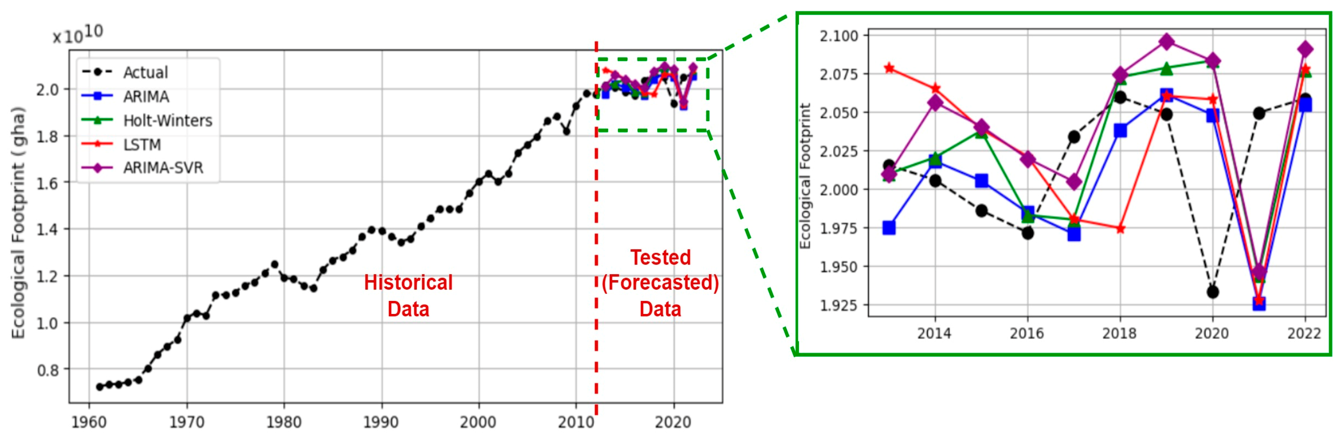Figure 7 illustrates forecasted EF values (10¹⁰ gha) by different time series models and actual EF values (10¹⁰ gha).

The zoomed-in section in Figure 7 displays the actual EF values (test set) for 2013–2022, along with the forecasted EF values by LSTM, ARIMA (1,1,0), Holt–Winters, and ARIMA-SVR for these years. Despite the growing inclination towards employing deep learning and hybrid methods for achieving more accurate forecasts, our findings demonstrate that the classical time series method ARIMA, known for its simplicity in implementation, yields more accurate EF forecasts compared to other methods.

The forecasting performances of the models were statistically tested using the Wilcoxon Signed-Rank and Friedman Tests. The significance level for both tests was set at 0.05. Thus, a robust statistical analysis of the models’ forecasting capabilities based on mean MAPE values was ensured. The results obtained from these tests are given in Table 7.

The Friedman test was employed to determine if there was a statistically significant difference among four different time series models. On the other hand, the Wilcoxon Signed-Rank Test was used to identify differences between pairs of models.

The Friedman test statistic yielded a statistic of 14.879, with a corresponding p-value of 0.0019. Since the p-value is <0.05, it is concluded that there is a statistically significant difference in the overall performance of the models. In the pairwise comparative analysis of forecasting models, according to the results of the Wilcoxon Signed-Rank Test, statistical differences emerged between several model pairs. Specifically, the ARIMA model exhibited statistically significant differences when compared to the ARIMA-SVR model (p = 0.00195), the Holt–Winters model (p = 0.00390), and between the ARIMA-SVR model and the Holt–Winters model (p = 0.00976).

These significant findings emphasize not only the overall importance of model performance but also highlight specific cases where one model performs better than another. The remarkable statistical discrepancy between the ARIMA model and both the ARIMA-SVR and Holt–Winters models (p = 0.00195 and p = 0.00390, respectively) signifies the ARIMA model’s superior predictive capabilities in comparison. Moreover, the notable difference observed between the ARIMA-SVR model and the Holt–Winters model (p = 0.00976) reveals specific aspects of performance, offering valuable insights into the strengths and weaknesses of each model. These results indicate that the ARIMA model stands out, demonstrating higher forecast accuracy and reliability compared to other models.

Advances in time series forecasting are characterized by innovative approaches, including the adoption of deep learning techniques, the use of big data, the widespread use of ensemble methods, and the integration of hybrid models in addition to classical time series methods. Moreover, increasing automation (especially automated software) has simplified model selection and parameter tuning, making them accessible to a wider range of users. These advancements have contributed to enhancing the precision, adaptability, and intelligibility of forecasting models [34,35].

Despite these advances, there are still fundamental challenges in forecasting time series. First, unexpected events and unusual circumstances can significantly affect forecasting models. For example, natural disasters, pandemics, or economic turmoil can make it difficult for models to understand past behavior and predict future trends. Second, accurately modeling nonlinear dynamics such as trends and seasonality in time series data is a challenge that is difficult to overcome using conventional methods [36]. Third, missing values can prevent the model from producing reliable forecasts, and data quality can significantly affect forecast accuracy [37]. Additionally, effective modeling of nonlinear relationships poses another major challenge in time series forecasting, along with technical challenges such as model selection and parameter tuning. Identifying the appropriate model and selecting suitable parameters requires a complex process.

The EF dataset used in this study presents two significant challenges. First, the analyzed data are highly non-stationary, making it difficult for time series models to effectively adapt to the non-stationary structures in the dataset. Second, the strict lockdowns imposed in 2020 due to the COVID-19 pandemic caused an unpredictable sudden drop in EF values. Anomalies (sudden decreases or increases) in datasets contradict previous data trends and patterns, making it difficult for models to make accurate predictions. Therefore, these sudden variations have a negative impact on the predictive performance of the models.

Forecasting sudden drops in real-world data is a challenging task for models. The substantial decrease in EF levels due to the closures caused by the COVID-19 pandemic in 2020 adversely affects the forecasting capabilities of the models. When assessing the model’s performance, it is essential to consider unforeseen circumstances of this nature. In this context, the EF forecasting errors of the time series models used in this study for the year 2020 were examined. Figure 8 illustrates the box-plot graph of the Mean Absolute Percentage Error (MAPE) results for the test set (2013−2022) for ARIMA (1,1,0), LSTM, ARIMA-SVR, and Holt–Winters models. All models forecast the EF amount in the year 2020 with higher errors compared to other years. However, the ARIMA (1,1,0) model achieved a more successful forecasting with a MAPE of 5.93%. Following that, the LSTM model had a MAPE of 6.44%, the ARIMA-SVR model had a MAPE of 7.73%, and the Holt–Winters model had a MAPE of 7.74%. These results indicate that the ARIMA model adapts better to unexpected situations. The lower forecasting errors demonstrate that the ARIMA model exhibits a more robust and reliable performance in Ecological Footprint (EF) forecasting, especially during extraordinary situations like COVID-19.

As a result, this study represents a significant step in evaluating the performance of time series models used in Ecological Footprint forecasting and understanding how they respond, particularly to unexpected events. The obtained results provide valuable insights for researchers in model selection and development.

When examining studies that forecast EF in the literature, it is observed that both a limited number of models are used, and the evaluation of model performances is based on the training set. Yao et al. [7] evaluated the dataset for the years 1999−2018 for training and assessed only ARIMA and GM based on the fitting performance criterion. Xu [9] only used the ARIMA-LSTM model. The model’s performance was tested on the training set, and MAE and RMSE values were displayed on the graph. Thus, the model’s performance was not tested on the test set, and no specific error value or rate was reported. Similarly, Jia et al. [10] only used the ARIMA model, and the model’s performance was presented graphically as actual, fitted, and residual values. No statistical metrics were provided for the performance of the ARIMA model on the test set. Wang et al. calculated MAPE and RMSE for the training dataset using ARIMA and ARIMA-ANN models. Liu et al. [6] performed EF predictions using different parameters as inputs. In this approach, using input parameters alongside time series improved the models’ prediction success. However, the study only tested 2 years (2014−2015). The most successful model, SVM, had an error rate of 1% for 2014 and 0.50% for 2015. However, the small size of the test set limits the models’ generalization ability. This situation makes it challenging for the results to gain overall validity and highlights a limitation that should be considered. Moros-Ochoa et al. [13] used Neural Network methods for EF and BC forecasting. The study reported the use of 11 NN methods for different parameters. MSE and MAE values for training and validation sets were graphically presented. Later, fishing grounds, grazing lands, forests, crops, built-up land, and carbon footprint values were forecasted for African, Asian, Central American, European, North American, Oceanian, and South American countries for the year 2030.

As a result, upon examining EF forecasting studies in the literature, it becomes apparent that a limited number of models were used, and the prediction performances of models with different structures have not been compared. In numerous studies, model performances were not assessed on the test or validation set. Focusing exclusively on training performance may prove inadequate for accurately evaluating a model’s real-world data performance. The evaluation of model performances through statistical analyses in studies is another noteworthy aspect. Additionally, the studies lack data containing anomalies such as COVID-19, and these anomalous situations remain unaddressed.

The distinctions of this study from others in the literature are outlined below:

• This study provides a comprehensive global ecological sustainability analysis using the worldwide total Ecological Footprint instead of specific geographical regions.
• It compares the forecasting performance of classical, deep learning, and hybrid time series models for the Ecological Footprint.
• The last 10 years, representing 15% of the time series dataset, have been used to evaluate the forecasting performance of the models. This approach allows for a more reliable assessment of how well the models perform under real-world conditions.
• The forecasting performances of the models have been assessed regarding the sudden decrease in Ecological Footprint due to COVID-19 lockdowns. Consequently, the capability of the forecasting models to handle anomalies in the datasets has been evaluated.

6. Conclusions

Forecasts of Ecological Footprint (EF) made with time series models enable the effective management of environmental impacts, the more efficient development of sustainability strategies, and the conscious utilization of existing resources. These forecasts contribute to a better understanding of environmental variability and aid in predicting future ecological impacts. As a result, sustainability efforts can be planned and implemented more effectively. Nevertheless, it is observed that there is a limited number of studies on EF forecasting using time series models in the literature. In this context, further comprehensive research is needed to identify models that will yield more successful results in this field.

This study compared deep learning, classical, and hybrid time series models to improve the accuracy of EF forecasting systems. As a result, based on the RMSE (42,452 × 10⁴ gha) and MAPE (2.12%) values for the test set, the ARIMA (1,1,0) model outperforms the LSTM, Holt–Winters, and hybrid ARIMA-SVR models. The superiority of the ARIMA (1,1,0) model has also been confirmed by the Wilcoxon Signed-Rank statistical test. However, owing to the effects of COVID-19 lockdowns, the global EF levels have deviated from their regular pattern. In this unexpected scenario of EF decrease, the forecasting errors of time series models have increased. Indeed, when EF forecasts for 2020 and 2021 are omitted, the MAPE value of the ARIMA model is 1.15%. This result indicates that anomalies in the dataset have a significant impact on the forecasting performance of the models. The findings suggest that the ARIMA model not only produces successful EF forecasts but also adapts better to unexpected situations.