
Characterization of a Transmon Qubit in a 3D Cavity for Quantum Machine Learning and Photon Counting

 , , , , , ,
  , , , , , , , , , , and
  add
Show full author list
add
Show full author list
Abstract
1. Introduction
2. Materials and Methods
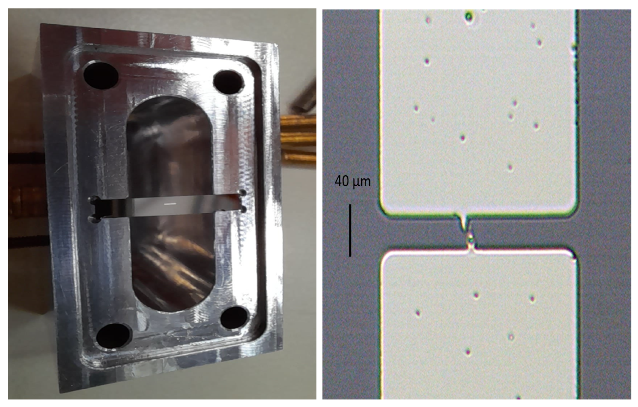
2.1. Transmon Fabrication
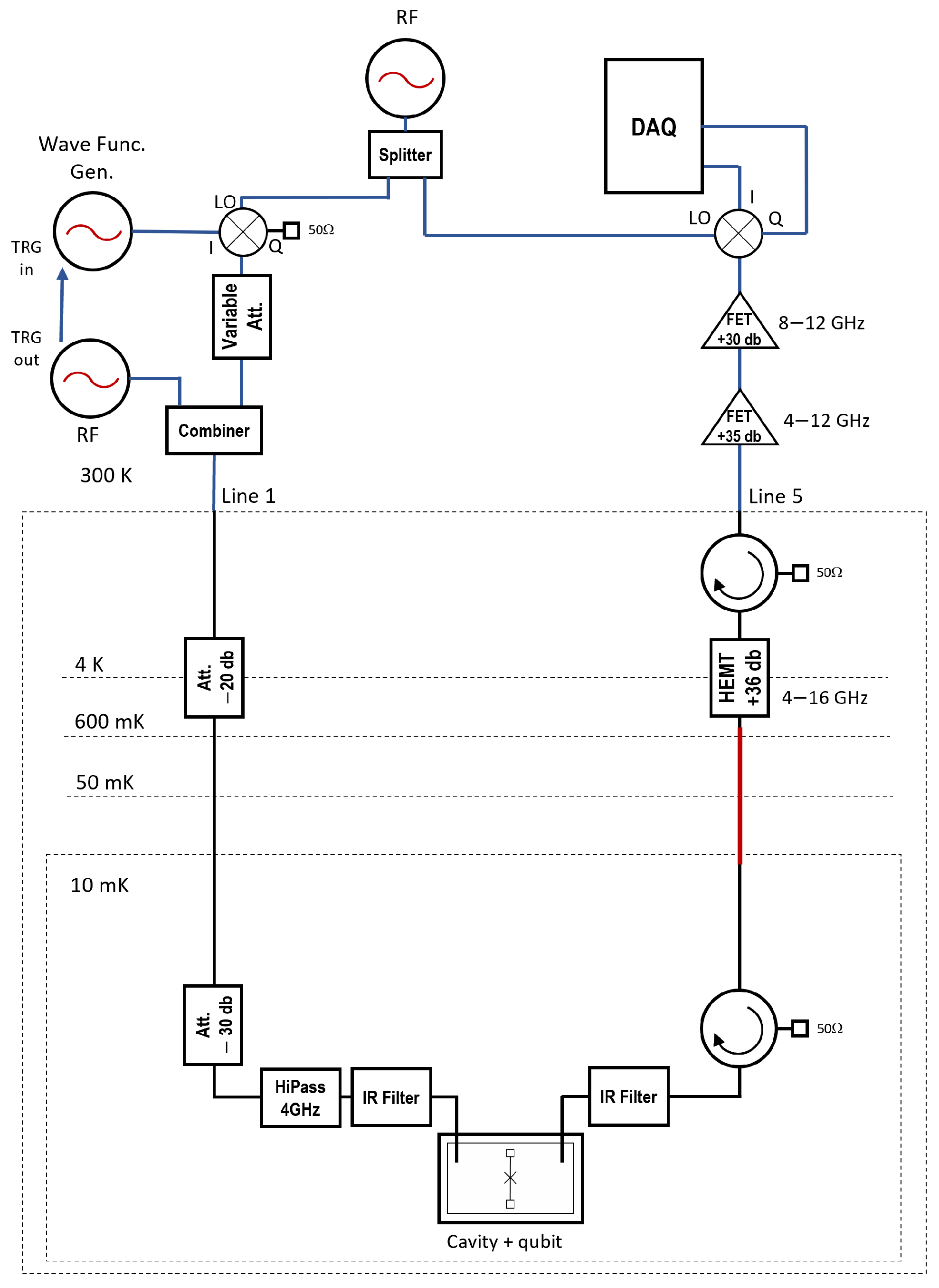
2.2. Experimental Setup for Transmon Characterization
3. Results
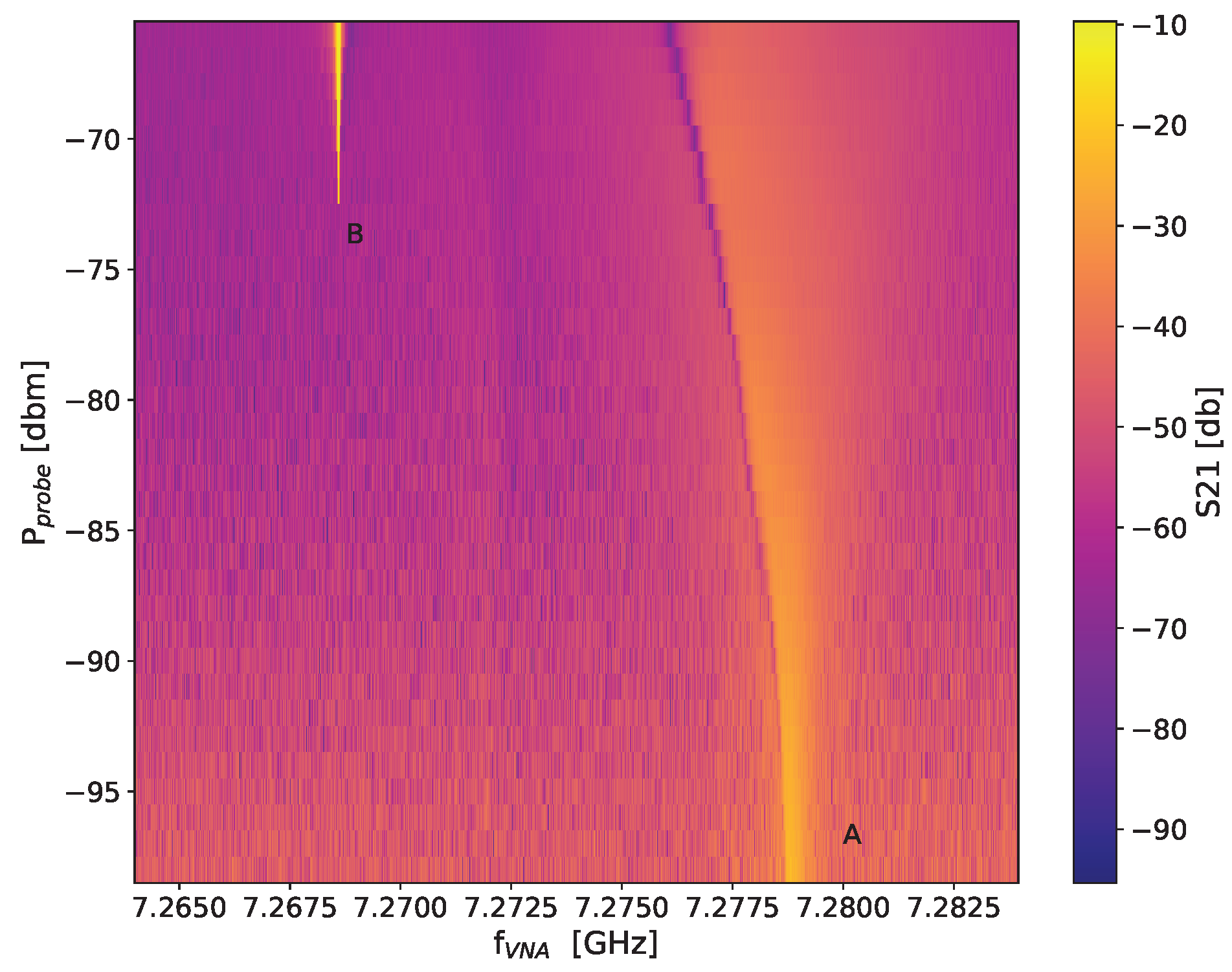
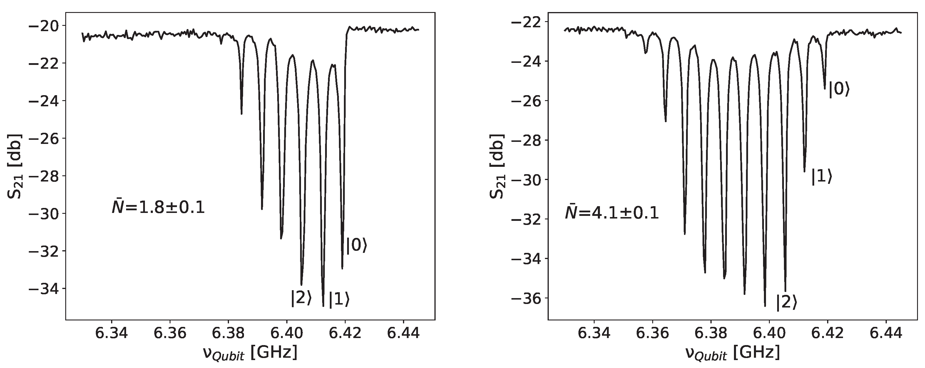
3.1. Transmon Spectroscopic Characterization
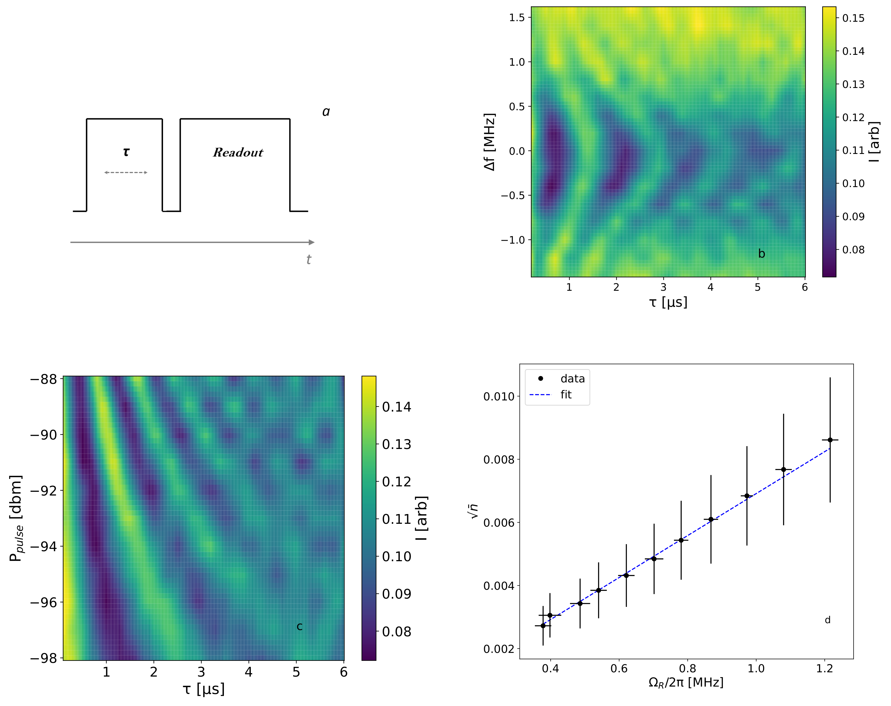
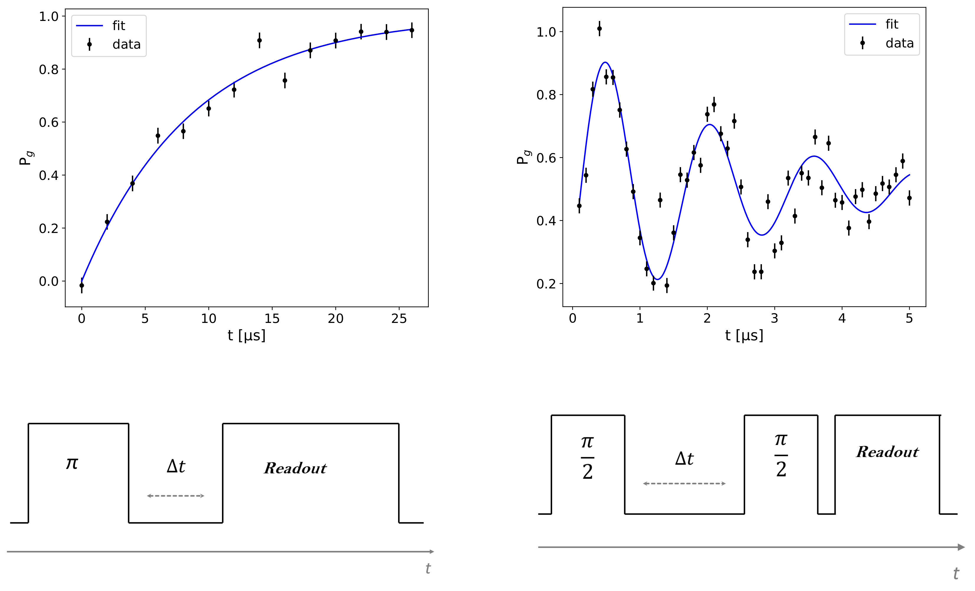
3.2. Time Domain Transmon Characterization
4. Simulation
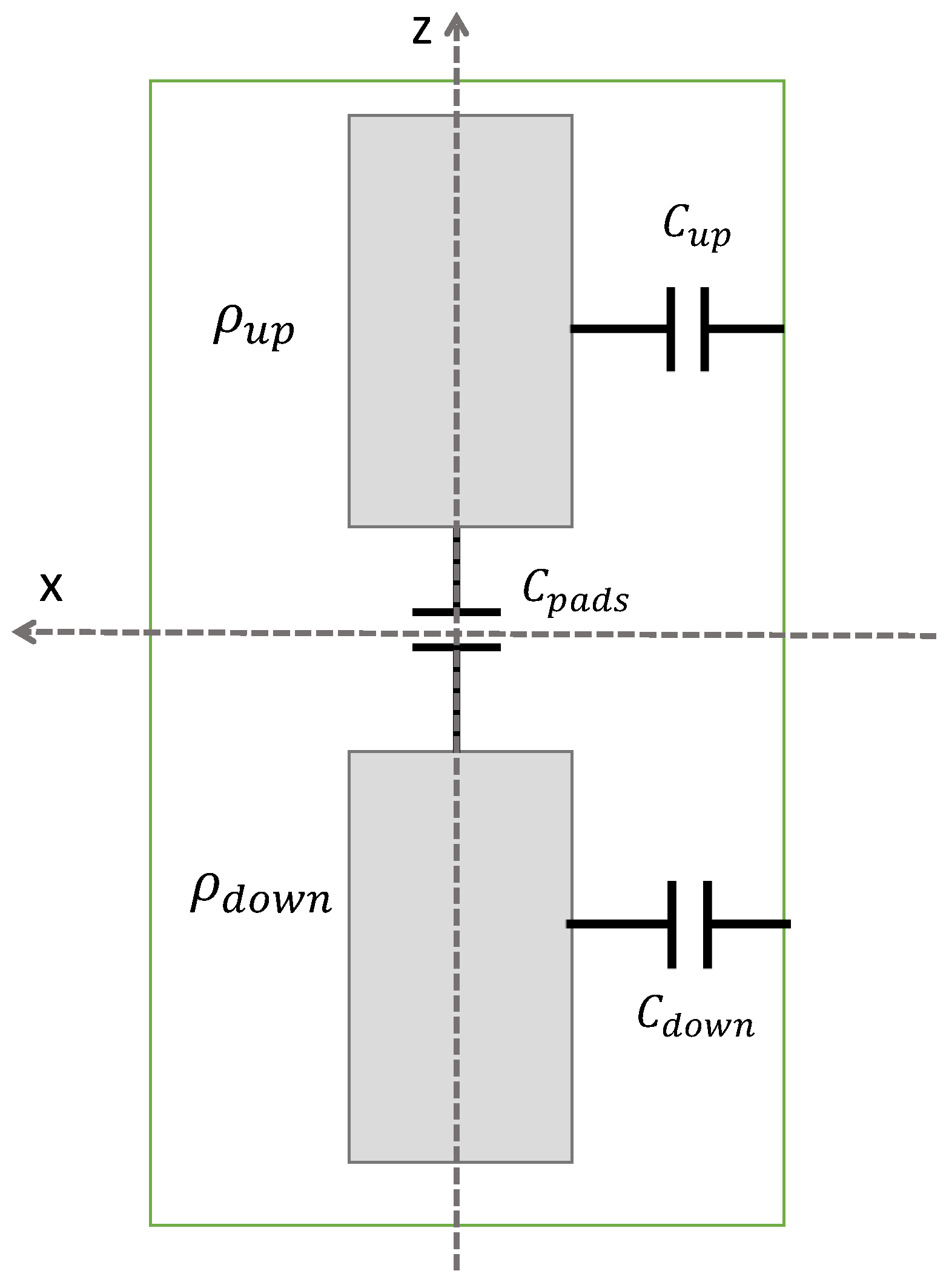
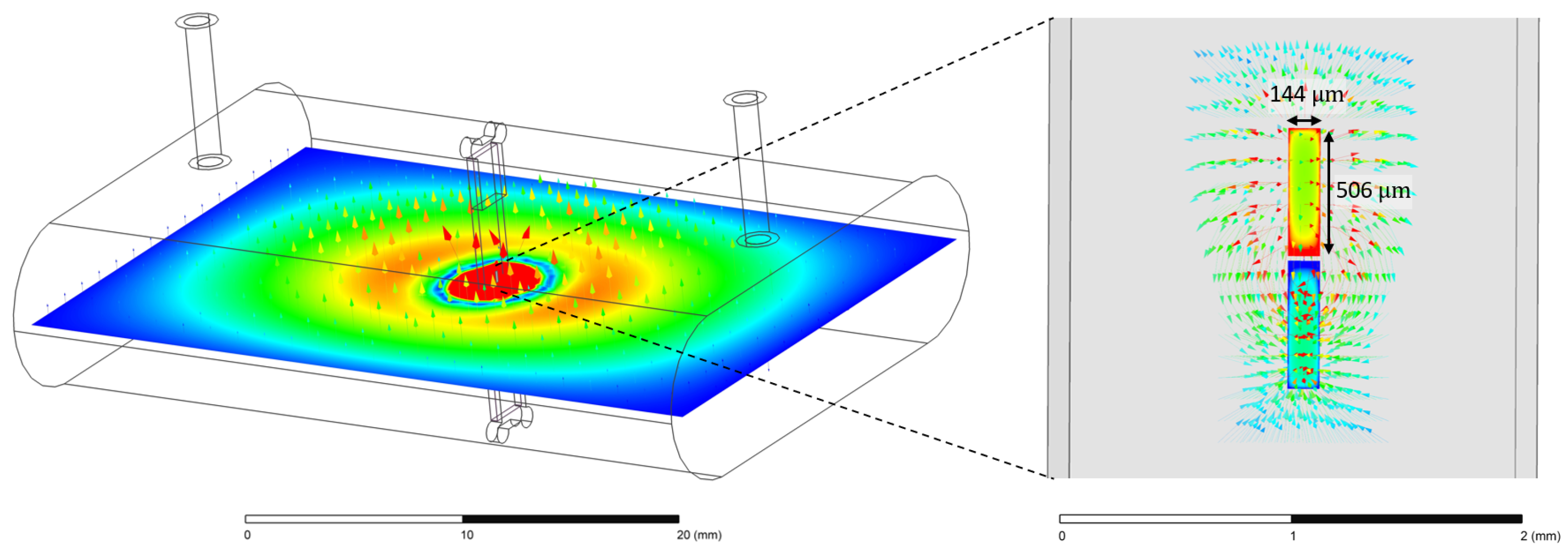
4.1. Capacitance
4.2. Dipole Coupling
4.3. Relaxation Time
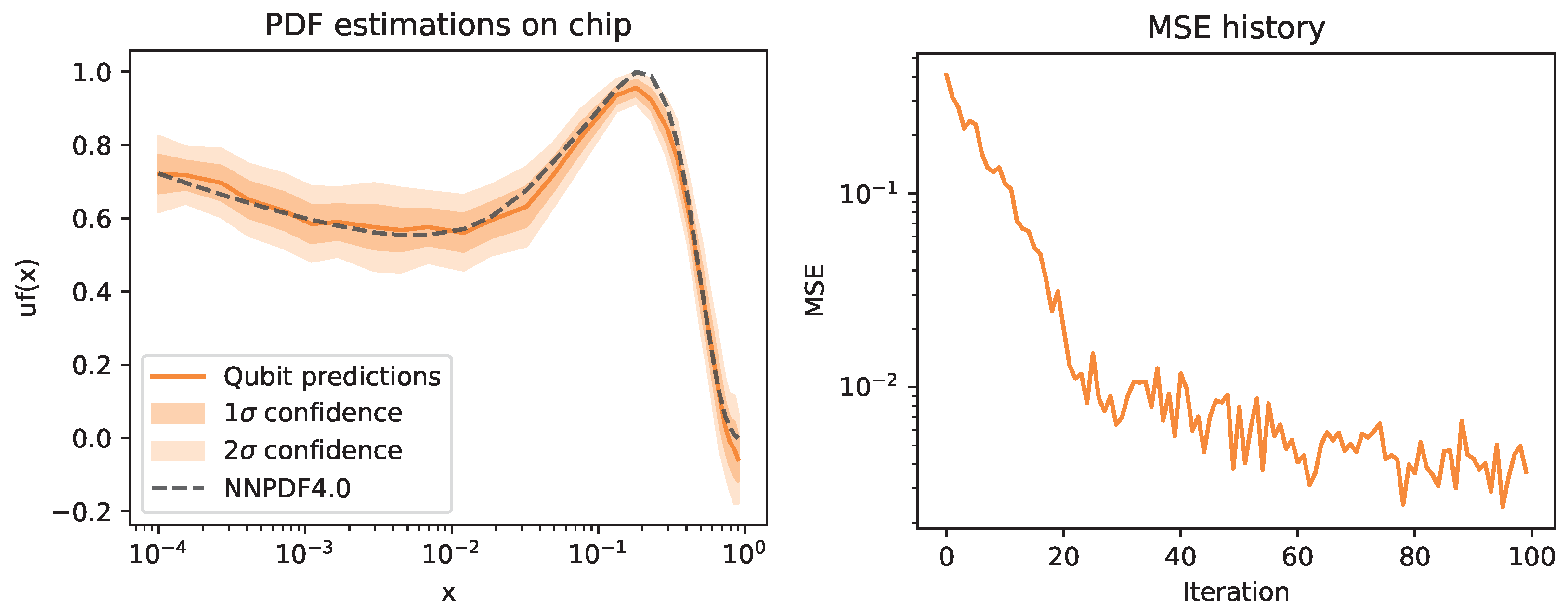
5. Fit to the -Quark Parton Distribution Function of the Proton with a Superconducting Transmon Qubit in a 3D Cavity
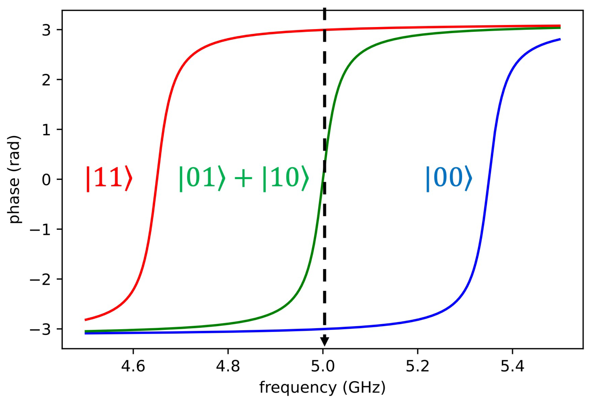
6. Measurement Protocol for a Low Dark-Count Photon Detector with Two Qubits
7. Conclusions
Author Contributions
Funding
Institutional Review Board Statement
Informed Consent Statement
Data Availability Statement
Acknowledgments
Conflicts of Interest
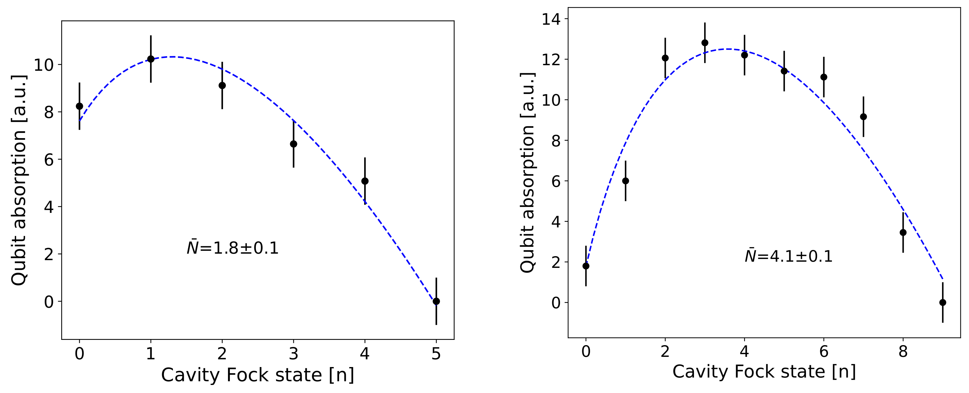
Appendix A. Average Photon Number inside the Cavity

Appendix B. Quantum Treatment of LC+Transmission Line

Appendix C. Capacitance Matrix and Total Capacitance
References
- Preskill, J. Quantum computing and the entanglement frontier. arXiv 2012, arXiv:1203.5813. [Google Scholar]
- Kjaergaard, M.; Schwartz, M.E.; Braumüller, J.; Krantz, P.; Wang, J.I.J.; Gustavsson, S.; Oliver, W.D. Superconducting qubits: Current state of play. Annu. Rev. Condens. Matter Phys. 2020, 11, 369–395. [Google Scholar] [CrossRef]
- D’Elia, A.; Rettaroli, A.; Tocci, S.; Babusci, D.; Barone, C.; Beretta, M.; Buonomo, B.; Chiarello, F.; Chikhi, N.; Di Gioacchino, D.; et al. Stepping closer to pulsed single microwave photon detectors for axions search. IEEE Trans. Appl. Supercond. 2022, 33, 1–9. [Google Scholar] [CrossRef]
- Rettaroli, A.; Alesini, D.; Babusci, D.; Barone, C.; Buonomo, B.; Beretta, M.M.; Castellano, G.; Chiarello, F.; Di Gioacchino, D.; Felici, G.; et al. Josephson junctions as single microwave photon counters: Simulation and characterization. Instruments 2021, 5, 25. [Google Scholar] [CrossRef]
- Golubev, D.S.; Il’ichev, E.V.; Kuzmin, L.S. Single-photon detection with a Josephson junction coupled to a resonator. Phys. Rev. Appl. 2021, 16, 014025. [Google Scholar] [CrossRef]
- Kono, S.; Koshino, K.; Tabuchi, Y.; Noguchi, A.; Nakamura, Y. Quantum non-demolition detection of an itinerant microwave photon. Nat. Phys. 2018, 14, 546–549. [Google Scholar] [CrossRef]
- Besse, J.C.; Gasparinetti, S.; Collodo, M.C.; Walter, T.; Kurpiers, P.; Pechal, M.; Eichler, C.; Wallraff, A. Single-Shot Quantum Nondemolition Detection of Individual Itinerant Microwave Photons. Phys. Rev. X 2018, 8, 021003. [Google Scholar] [CrossRef]
- Inomata, K.; Lin, Z.; Koshino, K.; Oliver, W.D.; Tsai, J.S.; Yamamoto, T.; Nakamura, Y. Single microwave-photon detector using an artificial Λ-type three-level system. Nat. Commun. 2016, 7, 12303. [Google Scholar] [CrossRef]
- Dixit, A.V.; Chakram, S.; He, K.; Agrawal, A.; Naik, R.K.; Schuster, D.I.; Chou, A. Searching for Dark Matter with a Superconducting Qubit. Phys. Rev. Lett. 2021, 126, 141302. [Google Scholar] [CrossRef]
- Lescanne, R.; Deléglise, S.; Albertinale, E.; Réglade, U.; Capelle, T.; Ivanov, E.; Jacqmin, T.; Leghtas, Z.; Flurin, E. Irreversible Qubit-Photon Coupling for the Detection of Itinerant Microwave Photons. Phys. Rev. X 2020, 10, 021038. [Google Scholar] [CrossRef]
- Butseraen, G.; Ranadive, A.; Aparicio, N.; Rafsanjani Amin, K.; Juyal, A.; Esposito, M.; Watanabe, K.; Taniguchi, T.; Roch, N.; Lefloch, F.; et al. A gate-tunable graphene Josephson parametric amplifier. Nat. Nanotechnol. 2022, 17, 1153–1158. [Google Scholar] [CrossRef] [PubMed]
- Aumentado, J. Superconducting parametric amplifiers: The state of the art in Josephson parametric amplifiers. IEEE Microw. Mag. 2020, 21, 45–59. [Google Scholar] [CrossRef]
- Macklin, C.; O’brien, K.; Hover, D.; Schwartz, M.; Bolkhovsky, V.; Zhang, X.; Oliver, W.; Siddiqi, I. A near–quantum-limited Josephson traveling-wave parametric amplifier. Science 2015, 350, 307–310. [Google Scholar] [CrossRef] [PubMed]
- D’ Elia, A.; Rettaroli, A.; Chiarello, F.; Di Gioacchino, D.; Enrico, E.; Fasolo, L.; Ligi, C.; Maccarrone, G.; Mantegazzini, F.; Margesin, B.; et al. Microwave Photon Emission in Superconducting Circuits. Instruments 2023, 7, 36. [Google Scholar] [CrossRef]
- Peugeot, A.; Ménard, G.; Dambach, S.; Westig, M.; Kubala, B.; Mukharsky, Y.; Altimiras, C.; Joyez, P.; Vion, D.; Roche, P.; et al. Generating two continuous entangled microwave beams using a dc-biased Josephson junction. Phys. Rev. X 2021, 11, 031008. [Google Scholar] [CrossRef]
- Esposito, M.; Ranadive, A.; Planat, L.; Leger, S.; Fraudet, D.; Jouanny, V.; Buisson, O.; Guichard, W.; Naud, C.; Aumentado, J.; et al. Observation of two-mode squeezing in a traveling wave parametric amplifier. Phys. Rev. Lett. 2022, 128, 153603. [Google Scholar] [CrossRef] [PubMed]
- Martinis, J.M. Superconducting phase qubits. Quantum Inf. Process. 2009, 8, 81–103. [Google Scholar] [CrossRef]
- Koch, J.; Terri, M.Y.; Gambetta, J.; Houck, A.A.; Schuster, D.I.; Majer, J.; Blais, A.; Devoret, M.H.; Girvin, S.M.; Schoelkopf, R.J. Charge-insensitive qubit design derived from the Cooper pair box. Phys. Rev. A 2007, 76, 042319. [Google Scholar] [CrossRef]
- Wang, C.; Li, X.; Xu, H.; Li, Z.; Wang, J.; Yang, Z.; Mi, Z.; Liang, X.; Su, T.; Yang, C.; et al. Towards practical quantum computers: Transmon qubit with a lifetime approaching 0.5 milliseconds. npj Quantum Inf. 2022, 8, 3. [Google Scholar] [CrossRef]
- Hyyppä, E.; Kundu, S.; Chan, C.F.; Gunyhó, A.; Hotari, J.; Janzso, D.; Juliusson, K.; Kiuru, O.; Kotilahti, J.; Landra, A.; et al. Unimon qubit. Nat. Commun. 2022, 13, 6895. [Google Scholar] [CrossRef]
- Gyenis, A.; Mundada, P.S.; Di Paolo, A.; Hazard, T.M.; You, X.; Schuster, D.I.; Koch, J.; Blais, A.; Houck, A.A. Experimental realization of a protected superconducting circuit derived from the 0–π qubit. PRX Quantum 2021, 2, 010339. [Google Scholar] [CrossRef]
- Bao, F.; Deng, H.; Ding, D.; Gao, R.; Gao, X.; Huang, C.; Jiang, X.; Ku, H.S.; Li, Z.; Ma, X.; et al. Fluxonium: An alternative qubit platform for high-fidelity operations. Phys. Rev. Lett. 2022, 129, 010502. [Google Scholar] [CrossRef] [PubMed]
- Reagor, M.; Paik, H.; Catelani, G.; Sun, L.; Axline, C.; Holland, E.; Pop, I.M.; Masluk, N.A.; Brecht, T.; Frunzio, L.; et al. Reaching 10 ms single photon lifetimes for superconducting aluminum cavities. App. Phys. Lett. 2013, 102, 192604. [Google Scholar] [CrossRef]
- Somoroff, A.; Ficheux, Q.; Mencia, R.A.; Xiong, H.; Kuzmin, R.; Manucharyan, V.E. Millisecond Coherence in a Superconducting Qubit. Phys. Rev. Lett. 2023, 130, 267001. [Google Scholar] [CrossRef] [PubMed]
- Joshi, A.; Noh, K.; Gao, Y.Y. Quantum information processing with bosonic qubits in circuit QED. Quantum Sci. Technol. 2021, 6, 033001. [Google Scholar] [CrossRef]
- Gao, Y.Y.; Rol, M.A.; Touzard, S.; Wang, C. Practical guide for building superconducting quantum devices. PRX Quantum 2021, 2, 040202. [Google Scholar] [CrossRef]
- Schuster, D.; Houck, A.A.; Schreier, J.; Wallraff, A.; Gambetta, J.; Blais, A.; Frunzio, L.; Majer, J.; Johnson, B.; Devoret, M.; et al. Resolving photon number states in a superconducting circuit. Nature 2007, 445, 515–518. [Google Scholar] [CrossRef] [PubMed]
- Blais, A.; Gambetta, J.; Wallraff, A.; Schuster, D.I.; Girvin, S.M.; Devoret, M.H.; Schoelkopf, R.J. Quantum-information processing with circuit quantum electrodynamics. Phys. Rev. A 2007, 75, 032329. [Google Scholar] [CrossRef]
- ANSYS, Inc. HFSS Fields Calculator Cookbook; Release 17.0; ANSYS, Inc.: Canonsburg, PA, USA, 2015. [Google Scholar]
- Miller, S. A Tunable 20 GHz Transmon Qubit in a 3D Cavity; Swiss Federal Institute of Technology Zurich: Zurich, Switzerland, 2018. [Google Scholar]
- Martinis, J.M. Surface loss calculations and design of a superconducting transmon qubit with tapered wiring. npj Quantum Inf. 2022, 8, 26. [Google Scholar] [CrossRef]
- Wenner, J.; Barends, R.; Bialczak, R.C.; Chen, Y.; Kelly, J.; Lucero, E.; Mariantoni, M.; Megrant, A.; O’Malley, P.J.J.; Sank, D.; et al. Surface loss simulations of superconducting coplanar waveguide resonators. Appl. Phys. Lett. 2011, 99, 113507. [Google Scholar] [CrossRef]
- Wang, C.; Axline, C.; Gao, Y.Y.; Brecht, T.; Chu, Y.; Frunzio, L.; Devoret, M.H.; Schoelkopf, R.J. Surface participation and dielectric loss in superconducting qubits. Appl. Phys. Lett. 2015, 107, 162601. [Google Scholar] [CrossRef]
- Cerezo, M.; Arrasmith, A.; Babbush, R.; Benjamin, S.C.; Endo, S.; Fujii, K.; McClean, J.R.; Mitarai, K.; Yuan, X.; Cincio, L.; et al. Variational quantum algorithms. Nat. Rev. Phys. 2021, 3, 625–644. [Google Scholar] [CrossRef]
- Pérez-Salinas, A.; Cruz-Martinez, J.; Alhajri, A.A.; Carrazza, S. Determining the proton content with a quantum computer. Phys. Rev. D 2021, 103, 034027. [Google Scholar] [CrossRef]
- Kingma, D.P.; Ba, J. Adam: A Method for Stochastic Optimization. arXiv 2017, arXiv:1412.6980. [Google Scholar]
- Mitarai, K.; Negoro, M.; Kitagawa, M.; Fujii, K. Quantum circuit learning. Phys. Rev. A 2018, 98, 032309. [Google Scholar] [CrossRef]
- Schuld, M.; Bergholm, V.; Gogolin, C.; Izaac, J.; Killoran, N. Evaluating analytic gradients on quantum hardware. Phys. Rev. A 2019, 99, 032331. [Google Scholar] [CrossRef]
- Mari, A.; Bromley, T.R.; Killoran, N. Estimating the gradient and higher-order derivatives on quantum hardware. Phys. Rev. A 2021, 103, 012405. [Google Scholar] [CrossRef]
- Schuld, M.; Sinayskiy, I.; Petruccione, F. An introduction to quantum machine learning. Contemp. Phys. 2014, 56, 172–185. [Google Scholar] [CrossRef]
- Biamonte, J.; Wittek, P.; Pancotti, N.; Rebentrost, P.; Wiebe, N.; Lloyd, S. Quantum machine learning. Nature 2017, 549, 195–202. [Google Scholar] [CrossRef]
- Robbiati, M.; Efthymiou, S.; Pasquale, A.; Carrazza, S. A quantum analytical Adam descent through parameter shift rule using Qibo. arXiv 2022, arXiv:2210.10787. [Google Scholar]
- Robbiati, M.; Cruz-Martinez, J.M.; Carrazza, S. Determining probability density functions with adiabatic quantum computing. arXiv 2023, arXiv:2303.11346. [Google Scholar]
- Cruz-Martinez, J.M.; Robbiati, M.; Carrazza, S. Multi-variable integration with a variational quantum circuit. arXiv 2023, arXiv:2308.05657. [Google Scholar]
- Robbiati, M.; Sopena, A.; Papaluca, A.; Carrazza, S. Real-time error mitigation for variational optimization on quantum hardware. arXiv 2023, arXiv:2311.05680. [Google Scholar]
- Efthymiou, S.; Ramos-Calderer, S.; Bravo-Prieto, C.; Pérez-Salinas, A.; García-Martín, D.; Garcia-Saez, A.; Latorre, J.I.; Carrazza, S. Qibo: A framework for quantum simulation with hardware acceleration. Quantum Sci. Technol. 2021, 7, 015018. [Google Scholar] [CrossRef]
- Efthymiou, S.; Ramos-Calderer, S.; Bravo-Prieto, C.; Pérez-Salinas, A.; García-Martín, D.; Garcia-Saez, A.; Latorre, J.I.; Carrazza, S. Quantum-TII/qibo: Qibo. Zenodo 2020. [Google Scholar] [CrossRef]
- Efthymiou, S.; Lazzarin, M.; Pasquale, A.; Carrazza, S. Quantum simulation with just-in-time compilation. Quantum 2022, 6, 814. [Google Scholar] [CrossRef]
- Efthymiou, S.; Carrazza, S.; Pasquale, A.; Mello, R.; Lazzarin, M.; Sopena, A.; Pedicillo, E.; vodovozovaliza. qiboteam/qibojit: qibojit 0.1.0. Zenodo 2023. [Google Scholar] [CrossRef]
- Efthymiou, S.; Orgaz-Fuertes, A.; Carobene, R.; Cereijo, J.; Pasquale, A.; Ramos-Calderer, S.; Bordoni, S.; Fuentes-Ruiz, D.; Candido, A.; Pedicillo, E.; et al. Qibolab: An open-source hybrid quantum operating system. arXiv 2023, arXiv:2308.06313. [Google Scholar]
- Pasquale, A.; Efthymiou, S.; Ramos-Calderer, S.; Wilkens, J.; Roth, I.; Carrazza, S. Towards an open-source framework to perform quantum calibration and characterization. arXiv 2023, arXiv:2303.10397. [Google Scholar]
- Carobene, R.; Candido, A.; Serrano, J.; Orgaz-Fuertes, A.; Giachero, A.; Carrazza, S. Qibosoq: An open-source framework for quantum circuit RFSoC programming. arXiv 2023, arXiv:2310.05851. [Google Scholar]
- Efthymiou, S.; Orgaz, Á.; Carobene, R.; Cereijo, J.; Carrazza, S.; Pasquale, A.; Simone-Bordoni; Sarlle, D.; Pedicillo, E.; maxhant; et al. qiboteam/qibolab: Qibolab 0.1.2. Zenodo 2023. [Google Scholar] [CrossRef]
- Pasquale, A.; Pedicillo, E.; Sarlle, D.; Efthymiou, S.; Cereijo, J.; Carrazza, S.; Vodovozovaliza; Orgaz, Á.; Sopena, A.; Candido, A.; et al. qiboteam/qibocal: Qibocal 0.0.4. Zenodo 2023. [Google Scholar] [CrossRef]
- Ball, R.D.; Carrazza, S.; Cruz-Martinez, J.; Debbio, L.D.; Forte, S.; Giani, T.; Iranipour, S.; Kassabov, Z.; Latorre, J.I.; Nocera, E.R.; et al. The path to proton structure at 1% accuracy. Eur. Phys. J. C 2022, 82, 428. [Google Scholar] [CrossRef]
- Majer, J.; Chow, J.; Gambetta, J.; Koch, J.; Johnson, B.; Schreier, J.; Frunzio, L.; Schuster, D.; Houck, A.A.; Wallraff, A.; et al. Coupling superconducting qubits via a cavity bus. Nature 2007, 449, 443–447. [Google Scholar] [CrossRef]
- Blais, A.; Huang, R.S.; Wallraff, A.; Girvin, S.M.; Schoelkopf, R.J. Cavity quantum electrodynamics for superconducting electrical circuits: An architecture for quantum computation. Phys. Rev. A 2004, 69, 062320. [Google Scholar] [CrossRef]
- Yurke, B.; Denker, J.S. Quantum network theory. Phys. Rev. A 1984, 29, 1419. [Google Scholar] [CrossRef]


| Variables | Values |
|---|---|
| [MHz] | −3.41± 0.08 |
| [MHz] | −10.2 ± 0.2 |
| [MHz] | −13.6 ± 0.3 |
| [MHz] | 421 ± 84 |
| [MHz] | 92.5 ± 1; 75 ± 12 |
| C [fF] | 46 ± 5 |
| [s] | 8.68 ± 0.72 |
| [s] | 2.30 ± 0.11 |
| [s] | 2.65 ± 0.15 |
| [nH] | 13 ± 2 |
| [nA] | 24.7 ± 1.3 |
| Variables | Values |
|---|---|
| 4.4 | |
| [s] | 156 |
| [s] | 57 |
| [s] | 42 |
| [fF] | 56 |
| [MHz] | 97 |
| Parameter | Optimizer | Inst. | |||||
| Value | 30 | 14 | Adam | 250 | ZCU111 |
Disclaimer/Publisher’s Note: The statements, opinions and data contained in all publications are solely those of the individual author(s) and contributor(s) and not of MDPI and/or the editor(s). MDPI and/or the editor(s) disclaim responsibility for any injury to people or property resulting from any ideas, methods, instructions or products referred to in the content. |
© 2024 by the authors. Licensee MDPI, Basel, Switzerland. This article is an open access article distributed under the terms and conditions of the Creative Commons Attribution (CC BY) license (https://creativecommons.org/licenses/by/4.0/).
Share and Cite
D’Elia, A.; Alfakes, B.; Alkhazaleh, A.; Banchi, L.; Beretta, M.; Carrazza, S.; Chiarello, F.; Di Gioacchino, D.; Giachero, A.; Henrich, F.; et al. Characterization of a Transmon Qubit in a 3D Cavity for Quantum Machine Learning and Photon Counting. Appl. Sci. 2024, 14, 1478. https://doi.org/10.3390/app14041478
D’Elia A, Alfakes B, Alkhazaleh A, Banchi L, Beretta M, Carrazza S, Chiarello F, Di Gioacchino D, Giachero A, Henrich F, et al. Characterization of a Transmon Qubit in a 3D Cavity for Quantum Machine Learning and Photon Counting. Applied Sciences. 2024; 14(4):1478. https://doi.org/10.3390/app14041478
Chicago/Turabian StyleD’Elia, Alessandro, Boulos Alfakes, Anas Alkhazaleh, Leonardo Banchi, Matteo Beretta, Stefano Carrazza, Fabio Chiarello, Daniele Di Gioacchino, Andrea Giachero, Felix Henrich, and et al. 2024. "Characterization of a Transmon Qubit in a 3D Cavity for Quantum Machine Learning and Photon Counting" Applied Sciences 14, no. 4: 1478. https://doi.org/10.3390/app14041478
APA StyleD’Elia, A., Alfakes, B., Alkhazaleh, A., Banchi, L., Beretta, M., Carrazza, S., Chiarello, F., Di Gioacchino, D., Giachero, A., Henrich, F., Piedjou Komnang, A. S., Ligi, C., Maccarrone, G., Macucci, M., Palumbo, E., Pasquale, A., Piersanti, L., Ravaux, F., Rettaroli, A., ... Gatti, C. (2024). Characterization of a Transmon Qubit in a 3D Cavity for Quantum Machine Learning and Photon Counting. Applied Sciences, 14(4), 1478. https://doi.org/10.3390/app14041478