A Remote Access Server with Chatbot User Interface for Coffee Grinder Burr Wear Level Assessment Based on Imaging Granule Analysis and Deep Learning Techniques

Featured Application

Remote coffee grinder burr wear level assessment system.

Abstract

Coffee chains are very popular around the world. Because overly worn coffee grinder burrs can downgrade the taste of coffee, coffee experts and professional cuppers in an anonymous coffee chain have developed a manual method to classify coffee grinder burr wear so that worn burrs can be replaced in time to maintain the good taste of coffee. In this paper, a remote access server system that can mimic the ability of those recognized coffee experts and professional cuppers to classify coffee grinder burr wear has been developed. Users only need to first upload a photo of coffee granules ground by a grinder to the system through a chatbot interface; then, they can receive the burr wear classification result from the remote server in a minute. The system first uses image processing to obtain the coffee granules’ size distribution. Based on the size distributions, unified length data inputs are then obtained to train and test the deep learning model so that it can classify the burr wear level into initial wear, normal wear, and severe wear with more than 96% accuracy. As only a mobile phone is needed to use this service, the proposed system is very suitable for both coffee chains and coffee lovers.

1. Introduction

Drinking coffee from chain coffee shops has become part of daily life for many people around the world. Therefore, chain coffee shops have great business opportunities and face great competition. The good quality control of coffee taste consistency is an important factor for chain coffee shops to win in the fierce competition present. The sharpness of the coffee grinder burr is recognized as an important factor affecting the flavor of coffee. Overly worn burrs can lead to under-extraction or over-extraction, resulting in sour or bitter flavors. Therefore, the grinding burr must be replaced in time to maintain the coffee flavor. However, the grinder burr should not be replaced too frequently or too early. Otherwise, it will increase the operating cost.

To precisely and directly measure the wear of coffee grinder burrs, professional engineers can examine their surface morphology using costly optical 3D profilometers and scanning electron microscopes. In industrial applications, noncontact detection or indirect measurement methods with acoustic emission sensing [1,2]; stray flux sensing [3]; and current, vibration, and force [4,5] are commonly used to measure cutting tool wear. A comprehensive survey of the sensor and signal processing systems in the machining process is available in [6]. Obviously, both the direct and indirect wear measurements for the cutting tools mentioned above are not only expensive but also difficult to carry out in coffee shops by employees who lack professional training. Therefore, those precision measurements can only be conducted in the laboratory by professionals. In this study, we worked with an anonymous but well-known coffee chain shop, which chose to remain anonymous due to commercial confidentiality considerations. Their experts and professional cuppers worked together to develop a manual method to categorize their grinder burr wear into initial wear, normal wear, and severe wear. The checking items include a quantitative analysis and qualitative analysis, such as visual inspection, texture of grounds, coffee granule size distribution [7], burr usage time, coffee extraction time, and taste. When a grinder burr is classified as severe wear, it needs to be replaced to maintain coffee taste. These checking items are actually related to each other, and checking them is very time-consuming. For example, workers have to use sieves or meshes to separate different coffee granule with different sizes to obtain the coffee granule size distribution. Measuring coffee granules is difficult because they are so small and numerous. For the coffee chains, the developed manual method to categorize their grinder burr wear is considered a commercial secret; therefore, they do not want to reveal it to the public, not even to the employees in their coffee chain shops. Because the methods include a qualitative analysis such as the taste of coffee based on years of professional experience, it is very difficult to educate their employees in chain shops to have a close ability, even if the coffee chains were willing to reveal the method. Therefore, the coffee chains came to us because they needed an automatic method to allow their employees to directly conduct the grinder burr wear checking in their coffee chain shops.

Because the cost of a target grinder burr is only about USD 150–200, and because the coffee chain has hundreds of stores, the coffee chains do not want to invest in in-store sensing or measurement equipment purchases and employee training because they do not want to solve a problem at the cost of invoking other potential problems of additional maintenance and training for new equipment. Therefore, the design challenge was to develop a system that automatically classifies coffee grinder burr wear with high accuracy within tight budget constraints. The brainstorming of building a workable system to meet the coffee chains requirements are as follows.

The checking items in the coffee chains’ manual method are actually correlated to each other. Among them, the coffee granule size distribution [7], obtained using sieves or meshes, is a quantitative analysis. Therefore, coffee granule size distribution is well suited as the input for the grinder burr wear prediction system because coffee granules are ground by the grinder burr with direct contact, consequently meaning that coffee granule sizes are directly affected by grinder burr wear. Image processing [8] that can separate the ground coffee granules and estimate their granule sizes is ideal for quickly obtaining coffee granule size distribution in coffee granule images.

The target coffee grinder of the cooperating coffee chain has five grinding settings. It was observed that the coffee granule size distributions of burrs with different wear levels and different grinding settings could be very similar to each other. Therefore, further intelligent processing of the coffee granule size distribution is needed so that the grinder burr wear level can be correctly assessed. A deep learning model [9,10] derived from neural networks is very suitable for handling this type of classification problem with ambiguity. If the input is the coffee granule size distribution while the output is the wear level of grinder burr, a deep learning model can be trained to classify the wear condition.

Because mobile phones and chatbots are now very popular, employees of coffee chain stores can use their mobile phones to take photos of grounded coffee granules and then submit the photos to a server computer for analysis through the chatbot messaging interface. After the analysis is complete, the wear prediction is sent back to employees through the same chatbot messaging interface. LINE [11] is a de facto messaging application in Taiwan and Asia. Therefore, a LINE bot was selected as the chatbot for this application.

In this paper, a system is developed using a chatbot messaging interface that allows users to interact with a server computer that is running an image processing and deep learning model, so that remote client users can first take photos of coffee granule and then submit images of coffee granules and text messages to the server computer to trigger burr wear classification programs and obtain analysis results.

With the above-proposed remote access server system, every coffee chain shop can replace the coffee grinder burr at the right time using the remote server that mimics the coffee experts’ abilities in classifying burr wear to maintain the good taste of coffee without extra implementation cost and training. Consequently, all of the design requirements from the coffee chains can be fulfilled.

To implement the proposed system, the following technical issues need to be addressed for a further detailed design.

The first technical issue is about a granule image acquisition device with a brightness control and scale calibration to establish a relationship between pixel sizes in the image and physical distances, as the coffee granule size distribution is the input to the deep learning model. Therefore, coffee granule sizes should be properly estimated. With the advancement in camera resolution, measuring the size of objects within images has become more precise and accessible. To accurately convert the sizes of objects in images to real dimensions, details about the camera parameters, as well as the angles and positions during capture, are essential [12]. To more effectively implement the proposed method, commonly encountered coins are applied as reference objects in images. In many applications, special image sampling devices are needed. The devices should be able to fix the shooting distance between the camera and the objects, control the ambient brightness during photography, and have a calibrate function to determine the scale of the image pixels to the actual length. For example, custom-built image-capturing platforms [13,14,15], microscopes with acquisition software [16,17,18,19], and high-resolution digital CCD industrial cameras with acquisition software [20] have brightness controls and known calibrated pixel to length ratios. In our case, for user convenience, by using a flash light, the coffee granule images are able to be taken by mobile phones at a distance roughly between 15 and 25 cm without precise pixel to length calibration. In our design, a simple and cost-free solution to overcome the scale calibration problem is to take photos of coffee granules and a reference coin with a known size [21] together under a flash light. Therefore, the coins and coffee granules in an image will be image processed together. At the end of the image processing, by measuring the coin of known size in the images, the real dimensions of other coffee granules can be calculated in the images because every coffee granule size can be estimated by multiplying the ratio of the pixel number of the coffee granule region to the pixel number of the reference coin by the actual size of the reference coin region.

The second technical issue is how to apply proper image processing techniques to separate the coffee granules from the background and estimate their sizes to obtain the coffee granule size distribution. In previous studies related to granule or particle segmentation, morphological watershed transform [8,22] processing has been successfully applied in the segmentation of solar photosphere particles [23,24], diagnostic systems to identify acute myeloid leukemia [16], granule segmentation in electron microscopy (EM) images [17], segmentation of biological membranes in electron tomography [25], fast imaging of yolk granules to quantify intraembryonic movement [18], evaluation of the particle size distributions of gravel [15] and on-site rockfill [26], DNA scalograms segmentation [27], and feature extraction of wear debris of planetary gearboxes [28]. Therefore, with so many successful results, the morphological watershed transform has also been selected for coffee granule segmentation in this paper. As a watershed transform is sensitive to noise, other case-dependent image processing operations should be properly performed to reduce noise before applying the watershed transform. The image pre-processing that needs to be performed before using a watershed transform generally includes image smoothing, background extraction [17], histogram equalization to enhance contrast [8], thresholding [16,17,23,24,29], and morphological operations [8,23,24,26,30], such as erosion, dilation, opening, closing to reduce noise, filling gaps, and enhancing or suppressing certain features based on their shape and size, making them useful for granule or particle segmentation. The distance transform is used to measure the distance of each pixel in an image to the nearest boundary. Using the distance image obtained from the distance transform [8,16,31] as an input for a watershed transform can improve the accuracy and control of the segmentation process. The image processing used in this paper will be explained in the details in the next section.

The third technical issue is how to build a deep learning model that can predict coffee grinder burr wear level with high accuracy. We should start with reviewing the recent progress of deep learning models. The paper in [32] provides a very comprehensive survey on image segmentation algorithms based on deep learning models.

The past decade was an era of technological leap forward in the development of artificial intelligence. A representative subject is AlexNet [33], proposed by Krizhevsky et al. They proposed convolutional neural network (CNN) architecture specifically designed for processing grid-like data, such as images and videos. CNNs consist of convolutional layers, pooling layers, fully connected layers, and an output layer. Among them, convolutional layers perform a dot product of the convolution kernel for obtaining feature maps; pooling layers to further downsample the feature maps, reduce its dimensionality, and retain the most important information; and fully connected layers for high-level reasoning and decision-making based on the extracted features. Since then, other improved and optimized methods inspired by AlexNet have been developed, such as VGG [34], ResNet [35], Inception [36], and so on. YOLO (You Only Look Once) [37] and the derived models are also CNN-based deep learning models designed for real-time object detection.

CNN and its derived methods can directly use images as inputs to train the deep learning model for classification applications, and it has become very popular in coffee-related applications. For example, the CNN-based or derived models have been successfully applied in coffee bean inspection machines [38], coffee bean quality screening [13], coffee bean defects [39,40], coffee leaf disease classification using ResNet50 [41] and MobileNetV3 [42], coffee maturity classification [43], and roasting coffee bean quality assessment using MobileNetV2 [44]. A good comparison of CNN-derived models is available in [44]. In addition, CNN-based methods have also worked well for particle size distributions (PSD)-related applications such as using YoLov5 to detect ore PSD [45] and using mask R-CNN (Regional CNN) to evaluate the PSD of on-site rockfill [26].

Although CNN-based methods using images as an input appear to be very effective and convenient to apply, annotations or labels are usually needed in the training and validation sets for object detection [26,45] and image classifications [13,39,40,41,42]. A comprehensive review on image segmentation algorithms based on deep learning models with annotated datasets is also available in [32].

However, in our case, across the hundreds of training and validation images, the coffee granules are much smaller and much more numerous than the ores of only 10–20 in training images in [45] using YoLov5; manual annotations are difficult and time-consuming. In addition, a convolutional neural network (CNN)-based method that downsamples images several times through convolution and pooling is not suitable for obtaining small coffee granule size information based on images from mobile phones. Furthermore, the size of flat images used as input vectors for deep learning models is quite large, which can result in very complex models that require better computers and more time for training. Therefore, we do not want to use CNN model and need to develop our image processing method and deep learning model.

On the other hand, another innovative technique proposed in AlexNet, such as the rectified linear unit (ReLU) activation function [46] and dropout [47], were adopted to build the deep learning model in this study, because the ReLU activation function alleviates the vanishing gradient problem, leading to faster convergence during training; a better learning of complex features and dropout involves randomly “dropping” (deactivating) a percentage of neurons during training, which encourages the network to learn more robust and general features.

The coffee experts provided us 600 coffee granule images taken by mobile phones upon our request. In the images, coffee granules were ground by all fifteen possible combinations of three different burr wear levels and five grinding settings. Each coffee granule image came with its label of the burr wear level. Therefore, we obtained a dataset of 600 images and partitioned it into training dataset of 480 images and validation dataset of 120 images. As every image is labeled, the deep learning model is trained in a supervised learning setting.

The deep learning model has also been applied on indirect tool wear prediction [29,48,49], not using images, but instead using physical signals such as force signals, vibration signals, acoustic emission signals, and current signals. In [48], a novel deep kernel autoencoder (DKAE) learning model used multichannel current signals fusion obtained from the current sensors of a three-axial computer numerical control (CNC) machine for tool wear recognition. The milling tool wear prediction method under variable working conditions based on the stacked autoencoder (SAE) network, which can adaptively extract tool wear features from the machining signal and a long short-term memory (LSTM) network of solving sequence problems and time correlation problems, is presented in [30]. Autoencoders [29,32,48] consist of an encoder and a decoder, and they aim to reconstruct the input data at the output layer. However, an autoencoder is a type of neural network architecture used in unsupervised learning. In [49], the study introduces a system-on-chip detection system using fusion signals from acoustic and vibrational sensors as inputs and a convolutional neural network (CNN) to predict the tool wear level of CNC machines. Those methods are not suitable in our case, because all of our training and validation images have been labeled. Therefore, we should still build a supervised deep learning model on our own.

Because we can decide how many size bins to use to divide the coffee granule size distribution, obtain granule counts for each size bin, and form the input vector for the deep learning model, we have additional design flexibility because the number of size bins is also the size of the input vector for the deep learning model. Using this method to obtain input vector provides some tolerance in the errors of granule size estimations. This is because the size errors mainly come from the noise reduction in image processing and should be small; even with size errors, most coffee granules still fall into the same size bins and may not affect the input vector of the deep learning model. In addition, as the deep learning model in this paper is for multi-class classification, its output are probability distributions rather than deterministic values. For a well-trained deep learning model, the predicted class is the one with the largest corresponding output probability, which is usually greater than the sum of the probabilities of the remaining classes. Therefore, the deep learning model allows for some input uncertainty due to coffee granule size errors without affecting the consistency of prediction.

In light of the above-mentioned literature review and evaluations for the detailed design, the combination of image processing, the deep learning model, and the LINE chatbot is the best integration for designing the proposed system, which meets the needs of coffee chains in terms of prediction accuracy, low cost, low system requirements, and user convenience.

2. Materials and Methods

In this paper, a deep learning model using unified granule size distribution obtained by proper image processing as an input is trained to mimic the ability of recognized coffee experts and professional cuppers to classify coffee grinder burr wear. Remote users only need to prepare one photo of coffee granules ground by their coffee grinder and upload the photo and send a text to the remote server computer through a chatbot messaging interface; the image process routine working using a deep learning model on the server computer can immediately classify the coffee grinder burr wear with high accuracy and can send the classification result back to the remote users. In this way, the coffee grinder burr wear identification capabilities of coffee experts can be extended to every coffee chain shop to maintain the same good taste of coffee. The complete design approach is explained in the following subsections.

2.1. Image Processing

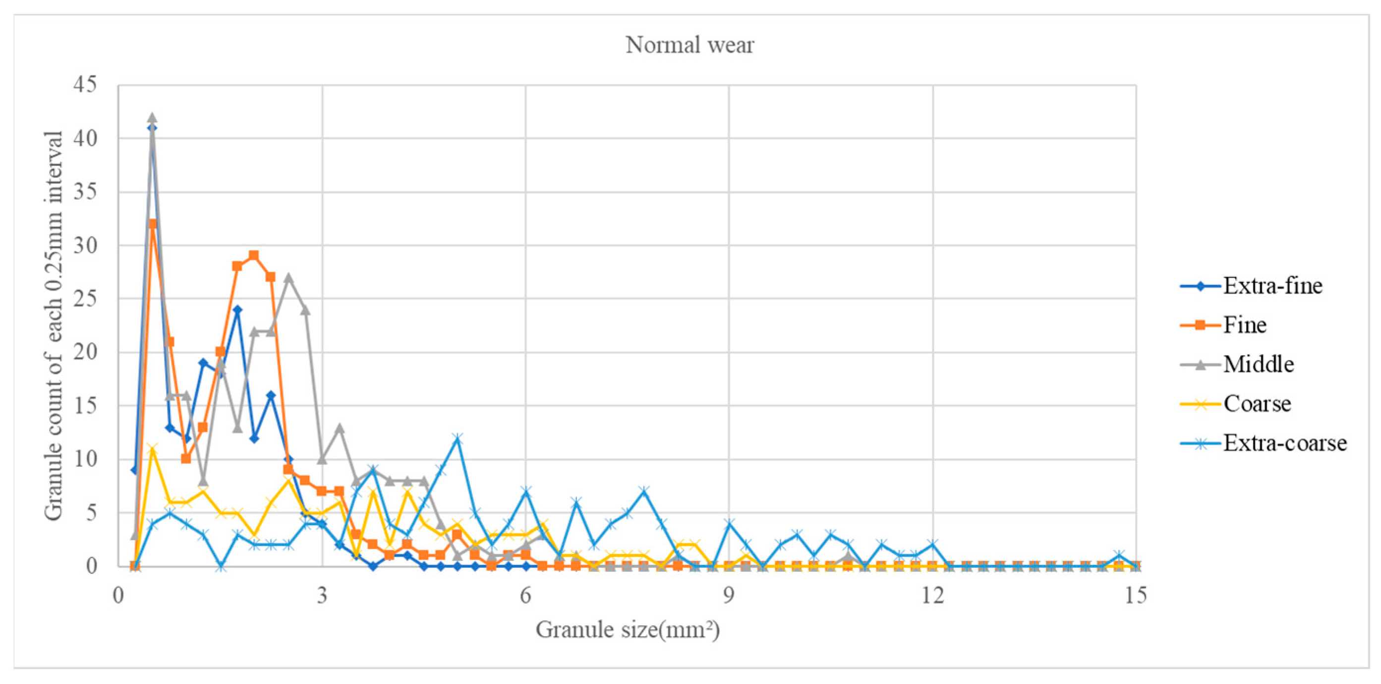
The chain stores’ coffee grinders have 5 grinding settings, such as extra-fine, fine, medium, coarse, and extra-coarse, which can grind a variety of different flavors of coffee. When a burr with a specific level of wear is installed, all 5 grinding settings on the coffee grinder are adjusted to collect the coffee granules produced at each setting. With 3 wear levels of grinder burr and 5 grinding settings, there are 15 grinding situations in total. By adjusting all 5 grind settings, several burrs with the same degree of wear were used to produce coffee granules. A total of 200 images of coffee granules with a size reference coin were collected for each burr wear level. Therefore, for 3 burr wear levels, 600 images in total were collected for image processing to extract unified granule size distributions for training and testing the deep learning model. To be able to operate conveniently inside the coffee shop, the following method, which does not require excessive accuracy, is used to prepare coffee granule images.

First, one grinds five coffee beans with the target coffee grinder and puts coffee granules on a white paper together with a size reference coin with a diameter of 20 mm. Then, one use the camera on a mobile phone with flash to take pictures of them at a distance of 20 cm plus or minus 5 cm to obtain the image. Using flash when taking photos at close range can make the ambient brightness more consistent. Therefore, a coffee shop clerk can easily prepare the image for the wear classification of grinder burrs.

In order to obtain the size distribution of coffee granules from the images, we need to perform a granule size distribution analysis in the image processing. As images of the coffee granules can be taken at different distances and angles, a coin with a known size is used as a reference to estimate every coffee granule size in all taken images and perform the image processing together.

When shooting, the coin is taken as a size reference in the image, so the actual area size of the coffee granules can be calculated from the proportional relationship between the actual area size of the coin and the number of pixels occupied by the coin in the image. For example, if a coin has an area of $100\pi {\mathrm{mm}}^2$ and occupies 100 pixels in the processed image, we know that the ratio of the number of pixels of the object in the processed image to the actual size of the object is $1:\pi$. Therefore, we can calculate each coffee granule area by multiplying the pixel number occupied by each coffee granule and $\pi$, as shown in Figure 1.

In practice, the coffee granules could overlap or touch each other or have tiny holes. To handle these mentioned problems, further noise reduction and morphological operations such as erosion, dilation, opening, and closing should be properly performed to process the images before they can be used to estimate coffee granule sizes.

The morphological operations [8] can be performed on both grayscale images and binary images. For grayscale images, the grayscale erosion [8] of an image involves assigning to each pixel the minimum value found over the neighborhood of the structuring element (kernel) to reduce the brightness. On the contrary, the grayscale dilation [8] of an image involves assigning to each pixel the maximum value found over the neighborhood of the structuring element; dilating bright regions also erodes dark regions. The grayscale opening [8] of an image involves performing a grayscale erosion followed by grayscale dilation to remove bright spots isolated in dark regions and to smooth boundaries; meanwhile, the grayscale closing [8] operation consists of a grayscale dilation followed by a grayscale erosion to remove dark spots isolated in bright regions and to smooth boundaries. For binary images, erosion [8] shrinking or thinning the white regions (foreground) while expanding the black regions (background) can be used to separate objects that are touching or overlapping; dilation [8] expanding or thickening the white regions (foreground) while shrinking or eroding the black regions (background) can be used to close gaps between objects or make them touch; opening [8] is a sequence of erosion followed by dilation to remove noise and small objects from binary images; and closing [8] is a sequence of dilation followed by erosion to close small gaps or holes in binary images. The mentioned morphological operations are applied interactively in further image processing. The first main step in image processing is to remove image background noise and create a mask that covers the regions of interest (ROIs) occupied by coffee granules and the reference coin in images. Then, we intersect the binary mask of ROIs, and the original image according to three color channels so that a color image will be obtained and both the coffee granules and the reference coin are extracted. The necessary steps are described in detail as follows.

First, we resize the original color image to a 3024 × 4032 resolution, converting it to an 8-bit grayscale image for further image processing. In a grayscale image, both the reference coin and the coffee granules are much darker than background. In other words, the pixel values of both the reference coin and coffee granules are much smaller than the pixel values of the background. The further image processing starts using a 500 × 500 round structuring element, which is larger than the scope of the reference coin and coffee granules, to perform grayscale dilation first followed by grayscale erosion so that both reference coin and coffee granules are eliminated and image background is extracted, as shown in Figure 2.

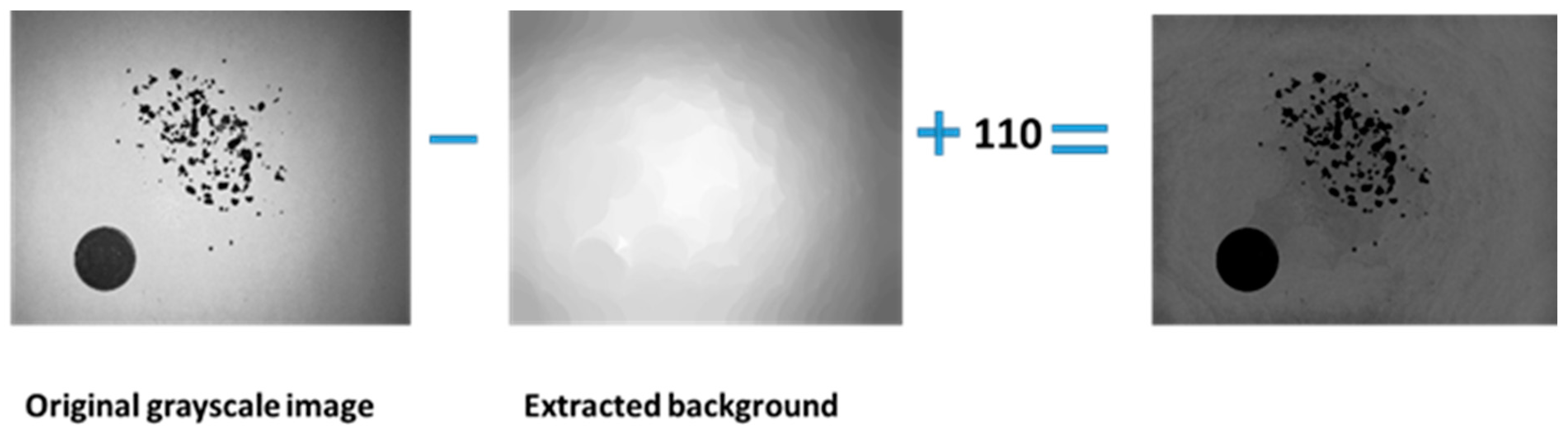
The main purpose of this operation is to average the background gray value of the original image so that the shadows are reduced, making it easier to extract the coffee granules and reference coin later. The original grayscale image is then subtracted from the extracted background grayscale image, and a grayscale bias is added. The bias is adjustable; in this case, the value is set to 110, aiming to isolate the regions occupied by the coffee granules and reference coin, as depicted in Figure 3. If an overflow or an underflow occurs, the pixel values are clipped.

Further processing includes performing a histogram equalization on the obtained image to increase the contrast between the coffee granules and the background, followed by reducing the noise using averaging filtering with a 5 × 5 mask on the image. Then, we use an 11 × 11 octagonal mask to successively perform grayscale closing to removes dark spots of tiny coffee powders isolated in the bright background and perform grayscale opening to fill bright spots of tiny holes isolated in dark coffee granules. In addition, coffee granule boundaries are smoothed. By conducting these tasks, more accurate shapes of coffee granules are obtained. To create the mask of the ROIs (the coffee granules and reference coin), the image is segmented using a global threshold with minimum value of 105 and a maximum value of 255. The process is illustrated in Figure 4.

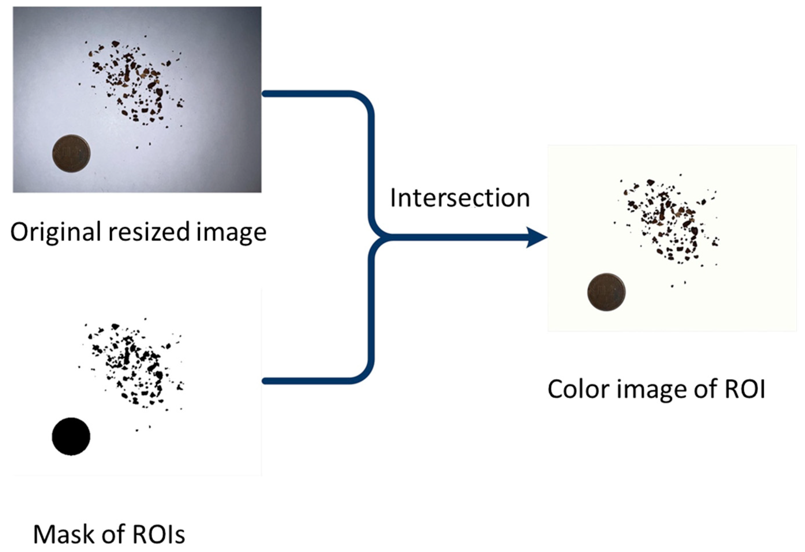
The obtained binary mask of the ROIs is then used to intersect with the original image according to three color channels so that a color image is obtained. Both the coffee granules and reference coin are extracted in black, and the bright background is now free of noise, as shown in Figure 5.

The second main step is to apply distance transformations [50] on coffee granule images to estimate coffee granule sizes. Distance images represent the distance of each pixel in the image to the nearest object boundary. These distance values are used to identify and segment coffee granule objects in the images. The steps to obtain the distance image include transforming the obtained color image of the ROIs in the previous step into a grayscale image, inverting the grayscale image, brightening the coffee grains and coin, and darkening the background, using an 11 × 11 octagonal mask to perform dilation to further close tiny gaps on the coffee granules, applying a global threshold with a minimum value of 100 and a maximum value of 255 to segment the image to obtain regions of interest (ROIs) for the coffee granules and reference coin, and performing distance transformations to change the pixel values inside the coffee granules or reference coin to their distances to the closest boundary. The complete processes for obtaining the distance image are illustrated in Figure 6.

The third main step is to apply a watershed transformation to the obtained distance images to further refine coffee granule boundaries for better segmentations. In the watershed transformation theory, an image is metaphorically treated as a topographic landscape, where the pixel intensities represent elevations. Low-intensity regions correspond to valleys, while high-intensity regions correspond to hills or peaks. The gradient of the distance image can help to identify the potential regions where watershed lines can be applied. Areas of large gradients with rapidly changing distance values usually correspond to object boundaries. The flooding typically starts from the local minima in the gradient image, corresponding to potential watershed lines. The threshold, which is the minimum height of the watersheds, should be set. Applying the watershed transform using the distance image and threshold as inputs can prevent over-segmentation, resulting in better segmentation results for images with complex structures and varied intensities. The algorithm simulates a flooding process, where it starts from the local minima and fills in regions based on the gradient information. Watershed lines separate different regions, and one can obtain segmented objects as distinct regions in the results. The detailed procedure of applying a watershed transform to segment coffee granules based on distance image is composed of performing a histogram equalization on the distance image to the full range of 0–255 to further enhance the size contrast of coffee granules, thereby obtaining a more accurate size distribution of coffee granules; inverting the distance image; performing a gray value closing with a small 3 × 3 rectangular mask on the inverted distance image to remove small holes so that the inverted distance image is clean, then performing a watershed transform to extract watershed basins from an image using a threshold of three for coffee granule segmentations; and finally calculating the intersection of the regions obtained in the watershed transform with the regions of interest (ROIs) in Figure 6 for the coffee granules and reference coin so that the coffee granules and reference coin are properly separated from the background. The above procedure is illustrated in Figure 7.

In the resulting image with the separated coffee granules and reference coin in Figure 7, calculating the pixel number within the scope of a coffee granule obtains the size of that coffee granule in the unit of pixels. The same method can also be used to obtain the size of the reference coin in the unit of pixels. As the sizes of those coffee granules are proportional to the size of the reference coin and the actual size of the reference coin is known, the size of every coffee granule is then calculated. Additionally, the total number of each coffee granule size is also calculated. Thus, a size distribution of coffee particles is obtained.

In the proposed image processing flow, morphological operations such as erosion, dilation, opening (erosion and dilation), and closing (dilation and erosion) can cause numerical propagation errors in the sizes of both the coffee granules and the reference coin in a preprocessed image and its processed image. The mean squared error (MSE) [8] and peak signal-to-noise ratio (PSNR) [8,28,51,52,53] can be used to calculate the errors between preprocessed images and processed images. The formula to calculate the MSE is as follows.

$$MSE(A,B)=\frac{1}{M\times N}{{\displaystyle \sum _{i=1}^M{\displaystyle \sum _{j=1}^N\left(A\left(i,j\right)-B(i,j)\right)}}}^2,$$

(1)

where:

• M is the number of rows in the images.
• N is the number of columns in the images.
• A(i,j) and B(i,j) are the pixel intensities at the corresponding locations in preprocessed images A and processed B.

A lower MSE indicates better similarity between the preprocessed image and processed image, as it implies that the pixel intensities are closer to each other. For an 8-bit grayscale image, its MSE ranges from 0 to ${255}^2\left(65025\right)$, where the lower, the better.

In addition to the MSE, the peak signal-to-noise ratio (PSNR) is another suitable metric for measuring the error between the preprocessed image and processed image. The PSNR is expressed in decibels (dB) and is calculated using the following formula:

$$PSNR=10\times {\log }_{10}\left(\frac{MAX}{MSE}\right),$$

(2)

where:

• MAX is the maximum possible pixel value of the image.
• MSE is the mean squared error, which is the average of the squared differences between the corresponding pixels of the original and processed images.

A PSNR value in the range of 20–30 dB usually indicates an acceptable level of distortion or noise in the processed image. PSNR values above 30 dB are often considered very good.

In the proposed image processing to obtain the size distribution of coffee granules, there are three main morphological operation steps that can cause errors for both the coffee granules and the reference coin in a preprocessed image and its processed image. A program was developed to calculate the MSE and PSNR for preliminary analysis.

The first step is the closing and opening operations with an 11 × 11 octagonal mask, performed on the averaging filtered image in the process to create the mask of ROIs, as shown in Figure 4. When test images were used, the obtained MSE and PSNR values were as follows.

MSE: 15.220496937200807

PSNR: 33.24 (dB) (very good)

The second step is the dilation operation with an 11 × 11 octagonal mask in the process to obtain the distance image as shown in Figure 6. When the same test images were used, the obtained MSE and PSNR values were as follows.

MSE: 9.238032495984505

PSNR: 20.31 (dB) (acceptable)

The third step is the closing operation with a 3 × 3 octagonal mask in the process of the watershed transform as shown in Figure 7. When the same test images were used, the obtained MSE and PSNR values were as follows.

MSE: 0.003990808321785505

PSNR: 72.12 (dB) (very good)

Those obtained MSE and PSNR values are either acceptable or very good at indicating that the errors caused by morphological operations are small. The reason is that when comparing with the 3024 × 4032 resolution of images, those 11 × 11 or 3 × 3 octagonal masks are very small. For the coffee granules that are relatively larger than the masks, when erosion and dilation occur in pairs and in succession, such as the operations of opening and closing, the net changes of pixels are small. The same goes for the reference coin. Therefore, those morphological operations mainly remove noise and fill small holes on coffee granules and do not cause obvious size errors in the preliminary analysis. Please keep in mind that the coffee granules and the reference coin underwent the proposed image processing together, so they both suffered from the same causes generating propagation errors. At the end of the image processing, every coffee granule size can be estimated by multiplying the ratio of the pixel number of the coffee granule region to the pixel number of the reference coin by the actual size of the reference coin region. The propagation errors of coffee granule sizes can be further reduced.

The effectiveness of the proposed image processing can be verified along with the deep learning model to see if their combination can successfully predict the grinder burr wear level, and this will be further discussed in next section.

2.2. Input Data Preprocessing for the Deep Learning Model Based on the Size Distribution of Coffee Granules

Because the coffee granule size distribution analysis is conducted to count the number of each granule size and the total number of different granule sizes, the input data vector of the deep learning model cannot be formed by simply using the numbers of each granule size as entries of the input data vector. Otherwise, the more different sizes of coffee granules that there are, the longer the input data vector length. Therefore, a reasonable data preprocessing is proposed to unify the number of inputs for the deep learning model. First, we divide the area sizes of all granules into N area size intervals from smallest to largest; then, we count the number of granules whose sizes fall into each area size interval so that the deep learning model has N inputs and each input is the total number of granules, whose area sizes fall into the corresponding area size interval. 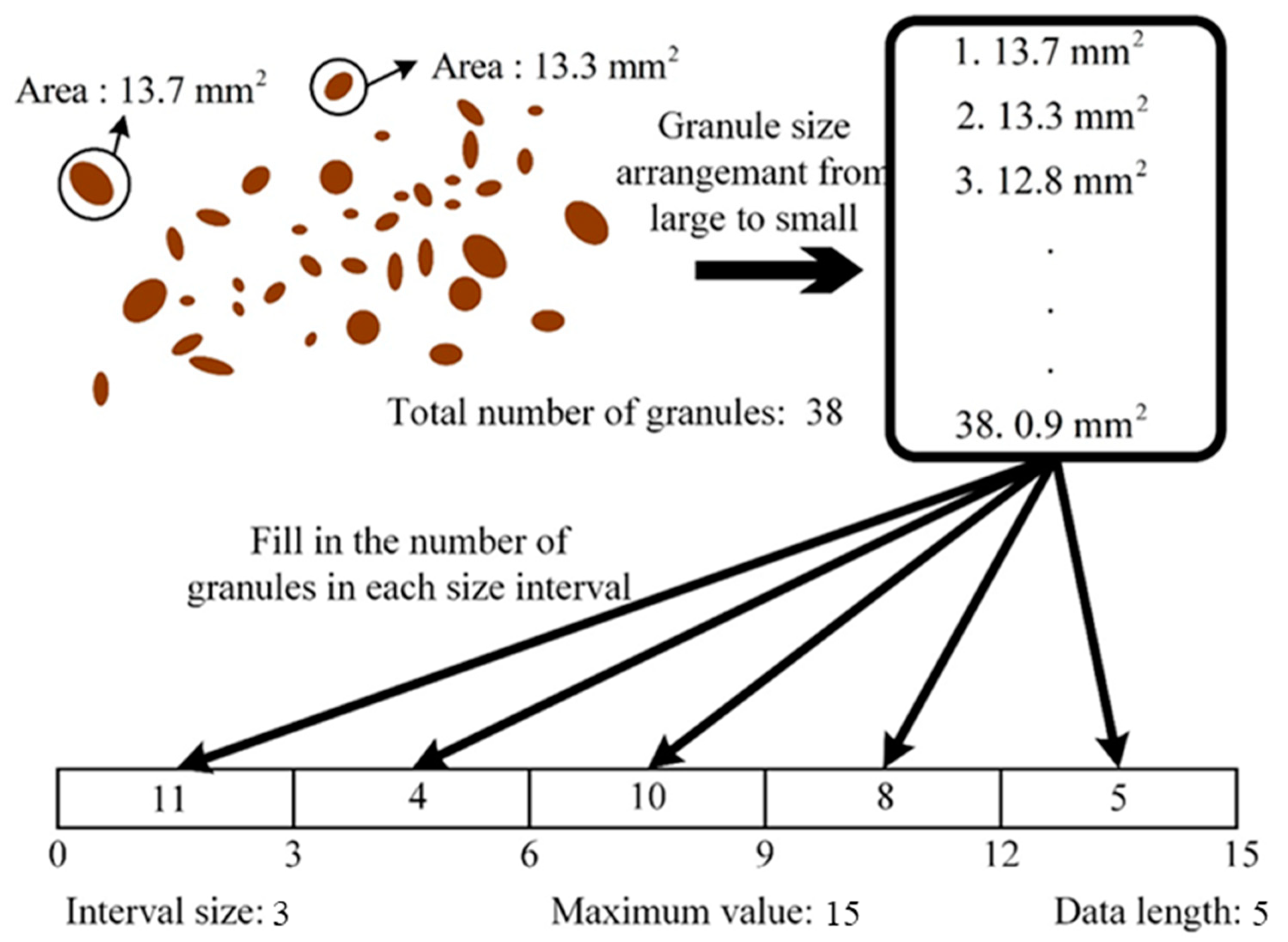Figure 8 illustrates the concept of unifying the number of inputs. There are 38 coffee granules in Figure 8, and the largest one is 13.7 mm². If the number of inputs is selected as N = 5, the interval size is $Roundup\left[\raisebox{1ex}{$13.7$}\!\left/ \!\raisebox{-1ex}{$5$}\right.\right]=3$. Then, the input vector is constructed using granule numbers in each size interval. In this case, the input vector x is as follows.

$$x={\left[\begin{array}{cccc}\begin{array}{cc}11& 4\end{array}& 10& 8& 5\end{array}\right]}^T$$

Therefore, the number of intervals chosen for the data segmentation of the coffee granule size distribution is the number of the input data for the deep learning model.

In addition, if the input data of the neural network for training are the quantities of granule sizes, it may not be able to converge or even diverge during training because some data may be too large. In order to prevent such problem, the input data are standardized with min-max normalization, as shown in (3).

$$x_{norm}=\frac{x-x_{\min }}{x_{\max }-x_{\min }}\in \left[0,1\right],$$

(3)

where $x_{norm}$ represents the normalized input value; $x_{\max }$ is the maximum value of all data; $x_{\min }$ is the minimum value of all data.

2.3. Introduction to Deep Learning Model

In this research, the coffee granule sizes and their distribution are the concerned features because the coffee chain regularly relies on using sieves or meshes to separate different coffee granule sizes and determine the relation between coffee taste and coffee granule size distribution. Other than burr wear classification, they also want to know if the image processing technique can obtain similar results of coffee granule size distribution. Therefore, a two-step approach is required, i.e., applying image processing to obtain the coffee granule size distribution and then using a deep learning model for burr wear classification.

The main purpose of training the deep learning model is to have high prediction accuracy. It is essential to strike a balance between model complexity and the available data, as overly complex models can lead to overfitting, while overly simple models may underfit the data. Multiple-layer deep learning models stem from neural networks. Neural networks consist of interconnected nodes called neurons, which are organized into input layers, hidden layers (zero or more), and output layers. The input layer receives the initial data, and the output layer produces the final result. Each connection between neurons has a weight associated with it. These weights determine the strength of the connection.

The activation function [46] is a nonlinear function that converts input signals into output signals in neural networks. The activation function introduces nonlinearity into the network, allowing it to learn complex patterns. Neurons in each layer receive inputs, apply the activation function to the weighted sum of those inputs, and pass the result to the next layer, as shown in Figure 9.

Neural networks learn by adjusting the weights of their connections to minimize the loss function during training iterations, allowing them to predict or classify a wide range of data.

Before training a deep learning model, one has to set up hyperparameters that are not learned from the training data but instead have to be predefined. In this research, Keras [54] in an open-source machine learning framework TensorFlow [55] are used to design, build, train, and deploy the deep learning model. A sequential deep learning model where one can stack layers one after the other to form a sequential flow of data is first created. The Adam (adaptive moment estimation) optimizer [56], which combines the advantages of both stochastic gradient descent (SGD) [56] and RMSprop (root mean square propagation) [57], is then used to compile the deep learning model. The Adam optimizer, which is often used as the default optimizer in many deep learning frameworks, including TensorFlow and Keras, has many advantages for training deep learning models such as effective default hyperparameters, adaptive learning rates, momentum-like updates, bias correction, and faster coverage speeds.

Finding the optimal deep learning architecture may require some trial and error in tuning the hyperparameters. The activation functions, number of inputs, number of neurons per layer, number of hidden layers, learning rates, and dropout rate [47] are the main hyperparameters for building the deep learning model.

As there are three burr wear level classifications, the problem handled in this paper is a multi-class classification problem. For a multi-class classification problem, the rectified linear unit (ReLU) in (4) and hyperbolic tangent function (tanh) in (5) are suitable candidates of activation functions of hidden layers to simulate nonlinear characteristics of this problem, while softmax in (6) is the choice for the activation functions of the output layer.

$$\mathrm{ReLu}\left(x\right)=\left\{\begin{array}{l}0 if x<0\\ x if x>0\end{array}\right., \mathrm{and} \mathrm{its} \mathrm{derivative} {\mathrm{ReLu}}^{\prime }\left(x\right)=\left\{\begin{array}{l}0 if x<0\\ 1 if x>0\end{array}\right.,$$

(4)

$$\tanh (x)=\frac{e^x-e^{-x}}{e^x+e^{-x}}, \mathrm{and} \mathrm{its} \mathrm{derivative} {\tanh }^{\prime }(x)=1-{\tanh }^2\left(x\right),$$

(5)

$$\sigma {\left(x\right)}_i=\frac{e^{x_i}}{{\displaystyle \sum _{j=1}^{j=3}{e}^{x_j}}} \mathrm{for} i=1,2,3 \mathrm{and} x={\left[\begin{array}{ccc}{x}_1& x_2& x_3\end{array}\right]}^T\in R^3,$$

(6)

The output layer of a neural network for three burr wear level classification with a softmax activation function will produce a probability distribution over the three classes. The softmax function takes a vector of arbitrary real-valued scores and converts them into probabilities. The output for each class is a value between 0 and 1, and the sum of the probabilities for all classes adds up to 1.

One-hot encoding is used in the neural network with three outputs to classify three different wear conditions of a grinder burr. When the burr is classified as severe wear, the encoding is 100; when the burr is classified as normal wear, the encoding is 010; and when the burr is classified as initial wear, the encoding is 001. The max probability in the output vector of the softmax function is the confidence score of the prediction.

In our multiple-class classification problem in deep learning, the model’s output is a probability distribution over the three classes. The most commonly used loss function for such problems is the categorical cross-entropy loss function (7), which quantifies the difference between the predicted probability distribution and the true distribution (one-hot encoded) of the classes.

$$L\left(y,p\right)=-{\displaystyle \sum _{i=1}^n{y}_i}\log \left(p_i\right),$$

(7)

where:

• y_i is the true probability distribution for the i-th sample (a one-hot encoded vector representing the true class).
• p_i is the predicted probability distribution for the i-th sample output by the model.

Dropout [47], which is to randomly “drop out” or ignore a proportion of neurons or units in a layer during each training iteration, is a regularization technique used in deep learning to prevent overfitting, which occurs when a model performs well on the training data but poorly on new, unseen data. Overfitting happens when a model becomes too complex and learns to memorize the noise in the training data rather than generalizing patterns that can apply to new data. Dropout is a simple yet effective way to address this issue.

Compared with directly using flattened images as the inputs for deep learning models in other applications, the inputs of the deep learning model in the proposed system are much smaller because the model uses a unified length vector based on the size distribution of coffee granules obtained from image processing. Therefore, we expect a deep learning model with a relatively simple architecture.

The proposed deep learning model design approach refers to the literature on the optimization of artificial neural network (ANN) parameters [58,59], and these methods are employed to set the number of hidden layers and neurons in the neural network for this study. The architecture of the neural network for this research is defined as follows:

$$\begin{array}{l}{z}_i^{\left(l+1\right)}=w_i^{\left(l+1\right)}{y}^l+b_i^{\left(l+1\right)},\\ y_i^{\left(l+1\right)}=f^l\left(z_i^{\left(l+1\right)}\right),\end{array}$$

(8)

where $l$ denotes the layer number,$y^{\left(l\right)}$ represents the output of layer $l$, $y^{\left(0\right)}$ is the input vector, $w$ and $b$ are the weight and bias values, $i$ is the neuron index within the hidden layer, and $f^l\left(\right)$ represents the activation function of layer $l$.

For simple deep learning models, a grid search [60,61] is a suitable method for finding the combination of hyperparameters.

The steps of the grid search are explained as follows.

First, we define a range of values or discrete options for each hyperparameter we want to tune. Second, we formulate all possible combinations of hyperparameter values to create a grid of configurations to be evaluated. Third, for each hyperparameter combination, we build and train a deep learning model using the training data. We evaluate the model’s performance according to the accuracy and speed of convergence to identify the best hyperparameter combination for the deep learning model. Fourth, we use a separate test dataset to ensure that the tuning process did not lead to overfitting to the validation data.

For the details of the deep learning models used in this study, please refer to “3.2 Building and Validating Deep Learning Model Architecture” to learn about its initial settings, hyperparameter tuning through grid search, comparison of different combinations of input sizes and activation functions, and assessment of the quality and accuracy.

2.4. Remote Access Server System with Chatbot User Interface for Classifying Grinder Burr Wear

To allow the remote client users to submit the coffee granule image and make an analysis request to the server computer to trigger image processing and deep learning model programs for burr wear classification and receive the analysis result in a convenient manner, a chatbot messaging interface that allows users to interact with the server computer has been developed. As LINE [11] is a de facto messaging application in Taiwan, LINE bot was selected as the chatbot for this application. LINE bots can respond to user messages and trigger actions on the application server according to user input.

The procedure of creating a LINE bot and connecting it to the application server is introduced as follows.

First, we browsed the LINE Developers website [62] to create a LINE Developer account.

Second, we created and configured a messaging API channel in LINE Developers. This channel will represent the LINE bot. In this step, a channel secret and channel access token are obtained and will be used to authenticate and authorize requests between the LINE bot and the application server.

Third, we downloaded and installed ngrok [63]. ngrok is a cross-platform, open-source software that provides a secure tunneling technology, allowing network traffic to be securely exposed to the public Internet. We ran ngrok to generate a public URL for the application server so that it became a public accessible web server to the LINE bot with the following command in the command window.

ngrok.exe http PORT_NUMBER

where PORT_NUMBER is the port number that the application server is listening in on.

Fourth, we used Node.js [64] and applied LINE API modules to create an execution environment that serves as a server so that users can send and receive text and image messages with the LINE bot and communicate with the messaging API.

Node.js, built on the V8 JavaScript engine developed by Google, is a JavaScript runtime that allows us to execute JavaScript code on the server side. It is known for its nonblocking, event-driven architecture, which makes it particularly well suited for building real-time applications of web servers. In the Node.js of this application server, the channel secret and channel access token of the LINE bot were specified, the server communication port number was set, and how the application server interactively handles and replies to the incoming users’ request messages was designed.

Fifth, we returned to the messaging API channel settings of LINE Developers to enter the generated application server URL using ngrok into the “Webhook URL” field to establish a secure tunnel between the LINE bot and the application server. To verify the webhook URL, LINE will send a GET request to the application server URL generated; the application server needs to handle this request to complete the verification. A webhook is a way for one system to provide real-time information to another system or application through HTTP POST requests.

Once the LINE bot and application server running image processing and deep learning model programs for burr wear classification are connected, the operational flow of how remote users can send coffee granule image and text message to application server and obtain the response of the grinder burr wear classification from the application server is given in Figure 10 below.

3. Experiment Results

3.1. Training and Test Data Preparation

For each burr wear level, the coffee experts use different burrs of the same wear level and adjust all five grind settings of the coffee grinder to produce coffee granules. For every burr level, 200 images were collected. Therefore, 600 images were collected for all three burr levels. Among them, 480 (80%) images were used for image processing to extract their granule size distribution. A total of 480 training data were then obtained by unifying the number of inputs and normalizing the range of the input data. Using the same processes, the remaining 120 images generated 120 test data. It was observed that when a grinding burr was using the extra-fine grind setting, the coffee granule size distribution was more concentrated than those using fine, medium, coarse, and extra-coarse grind settings. Basically, the coarser the grind setting, the less concentrated the coffee granule distribution and the lower the granule count in every interval, as shown in Figure 11, Figure 12 and Figure 13. This is because even if a coarse grind setting is used, some fine coffee granules are still inevitably produced to enlarge the scope of the coffee granule size distribution.

It was found in experiments that grinder burrs with different wear levels could produce similar coffee granule size distributions when using different grind settings. For example, the coffee granule size distribution of a severely worn burr with the extra-coarse grind setting are very similar to that of an initial wear burr with the extra-fine grinding setting, as shown in Figure 14. This phenomenon can easily lead to people misjudging the wear level of the burrs, and that is why the deep learning model is needed for more accurate burr wear level classifications.

3.2. Building and Verifying the Deep Learning Model Architecture

In the preliminary setup of the deep learning model of this research, the Adam in Keras [54] was selected as an optimizer for avoiding a potential local minimum because the learning rate is adjusted automatically during training. The ReLU in (4), which has no vanishing gradient problem, was used as the activation function of neurons in hidden layers, while softmax was used as the activation function of neurons in the output layer. Using images in training dataset, the granule size distributions obtained from the proposed image processing was divided into 16 intervals to form the inputs.

As the size of default input vectors is small, only 16 × 1, the expected deep learning model should be simple. A grid search [60,61] was conducted to select the rest of the hyperparameters in the deep learning model. A grid search exhaustively tries every possible combination to determine the best set of hyperparameters. We used the following hyperparameter grid in

Table 1. Hyperparameter grid.

No. of Neurons	No. of Hidden Layers	Batch Sizes	Epochs	Dropout Rates
16, 32, 64	2, 3	16, 32, 64	500, 1000	0.2, 0.3

and aimed to obtain a preliminary deep learning model with a prediction accuracy of over 80%.

An epoch refers to one complete pass through the entire training dataset. During each epoch, the model sees and learns from all training samples once. Batch size refers to the number of training examples utilized in one iteration. In other words, it defines the number of samples that will be propagated through the neural network before updating the model parameters (weights and biases). Smaller batch sizes can introduce some randomness into the training process and might help the model generalize better. Because we have 480 training datapoints, the three batch size options are well below 480. Large epochs might be helpful for obtaining high accuracy but might result in overfitting for the test data. Therefore, dropout that can prevent or reduce overfitting was also considered.

A simple grid search can be conducted manually. There is also software available for performing complex grid searches. For example, GridSearchCV [61] is a hyperparameter-tuning function provided by the Scikit-learn library [65] in Python, specifically within the model_selection module. It systematically searches for a predefined set of hyperparameters and evaluates the model performance for each combination. KerasClassifier [66] is a wrapper class in the Keras library that allows us to use Keras models with Scikit-learn’s GridSearchCV. By combining KerasClassifier with GridSearchCV, one can easily tune hyperparameters for deep learning models built using Keras.

After the grid search, a preliminary 5-layer deep learning model includes an input layer, an output layer using softmax as the activation function, and 3 hidden layers using the ReLu as the activation function, with 64 neurons, 32 neurons, and 16 neurons, respectively, being selected because it has acceptable accuracy and convergence speed. Its batch size is 32 and epoch number is 1000. In addition, the first two hidden layers had a 0.3 dropout rate to prevent overfitting on the test data. However, when running the preliminary deep learning model with validation data, the confidence scores were still lower than the confidence scores in training. This means that the model was overly trained and overfitting still occurred. After we manually increased the dropout to 0.5 (50%), the overfitting was reduced because the confidence scores for training and testing were very close to each other.

This study focuses on investigating the impact of interval separation for different input quantities on classification accuracy; a three-layer hidden layer is employed as the experimental framework. Through a grid search, the hidden layers $y^{\left(1\right)}$, $y^{\left(2\right)}$, and $y^{\left(3\right)}$ are set to possible maximum neuron quantities of 64, 32, and 16, respectively, ensuring that the neural network can accurately classify inputs. This setup facilitates the study in handling varying quantities of input vectors. Simultaneously, for a dropout rate vector denoted as $r$, for each neuron $j$ within each layer $l$, a probability $p$ is stochastically generated using a Bernoulli distribution, which is expressed as follows,

$$r_j^{\left(l\right)}\sim Bernoulli\left(p\right),$$

(9)

The Bernoulli distribution is a random process to create the dropout mask (the binary mask applied to the input units), where each unit has a certain probability p of being “dropped out” (set to zero).

The network with the dropout mechanism can be redefined as follows,

$$\begin{array}{l}{\tilde{y}}^{\left(l\right)}=r^{\left(l\right)}\ast y^{\left(l\right)},\\ z_i^{\left(l+1\right)}=w_i^{\left(l+1\right)}{\tilde{y}}^{\left(l\right)}+b_i^{\left(l+1\right)},\\ z_i^{\left(l+1\right)}=f^{\left(l\right)}\left(z_i^{\left(l+1\right)}\right),\end{array}$$

(10)

where $l$ denotes the layer number, $y^{\left(l\right)}$ represents the output of layer $l$, $y^{\left(0\right)}$ is the input vector, $w$ and $b$ are the weight and bias values, $i$ is the neuron index within the hidden layer, and $f^{\left(l\right)}\left(\right)$ represents the activation function of layer $l$.

As the dropout mechanism can selectively deactivate the activation function of neurons during the prediction process, it supports the network to prevent overfitting.

Further fine tuning was conducted to determine the number of intervals for data segmentation based on the coffee granule size distribution and the choice of activation function. The granule size distributions obtained from the same image, divided into four different intervals: 16, 21, 31, and 61, are given in Figure 15.

As shown in Figure 15, when the interval length is 61, the coverage range is denser, and its characteristics have obvious fluctuations; when the interval length is 16, the coverage range is wider, and the fluctuations of its characteristics are relatively gentle.

Therefore, the number of intervals affects the characteristics of the model input data. In order to find the appropriate number of intervals, we must conduct experimental comparisons of different numbers of intervals.

The initial activation function ReLU can be regarded as an equal function of positive input, and it always maintains a gradient of one, so it can improve the vanishing gradient problem of deep learning models. However, for negative input values, the output of ReLU and its gradient are always zero, which causes the weights to not be updated when the input value is negative. In order to know whether ReLU is still a good choice for the hidden layers of this deep learning model, the experiment also used tanh in (5) as another activation function to compare with ReLU in detail.

In order to improve the detectability of the training results, the training and test sets were redistributed five times, resulting in a total of five sets of training results for comparison. Such a method can reduce the impact of accidental factors on training results and increase the stability and reliability of the model.

When the trained deep learning model used ReLU as the activation function, the training results of four different intervals used as the input number are given in

Table 2. Training accuracies using ReLU and four different interval numbers.

Interval Numbers	Group 1	Group 2	Group 3	Group 4	Group 5	Average
16	94%	96%	93%	95%	98%	95.2%
21	96%	99%	97%	97%	99%	97.6%
31	100%	100%	98%	100%	100%	99.6%
61	100%	100%	100%	100%	100%	100%

, and the test results are given in

Table 3. Test accuracies using ReLU and four different interval numbers.

Interval Numbers	Group 1	Group 2	Group 3	Group 4	Group 5	Average
16	97%	98%	97%	98%	92%	96.4%
21	96%	98%	96%	99%	92%	96.2%
31	97%	98%	98%	98%	94%	97%
61	98%	96%	98%	95%	92%	95.8%

. It is observed from these results that no matter which interval is used, the accuracy of training as well as testing reached more than 95%.

From Table 1 and Table 2, it is observed that the training accuracy of 61 intervals is higher than that of 31 intervals, while the test accuracy of 61 intervals is lower than that of 31 intervals. Therefore, using 61 intervals could result in slight overfitting.

The convergence speeds of accuracies of using four different intervals can also be observed from Figure 16. The accuracy convergence of 31 intervals and 61 intervals are very fast and close to each other.

Table 4. Interval numbers vs. total parameters.

Interval numbers	16	21	31	61
Total Parameters	3747	4067	4707	6627

gives the numbers of parameters of models built using different intervals to process the granule size distribution as the input for the deep learning model. It is obvious that the larger the numbers of intervals, the larger the total parameters, and consequently the more complex the deep learning model.

When the trained deep learning model used tanh as the activation function, the training results of four different intervals used as the input are given in the

Table 5. Training accuracies using tanh and four different interval numbers.

Interval Numbers	Group 1	Group 2	Group 3	Group 4	Group 5	Average
16	92%	88%	91%	91%	92%	90.8%
21	90%	91%	88%	90%	94%	90.6%
31	94%	94%	94%	96%	96%	94.8%
61	98%	96%	98%	96%	97%	97%

, and the test results are given in

Table 6. Test accuracies using tanh and four different interval numbers.

Interval Numbers	Group 1	Group 2	Group 3	Group 4	Group 5	Average
16	92%	95%	92%	97%	88%	92.8%
21	91%	92%	89%	94%	86%	90.4%
31	92%	93%	92%	94%	88%	91.8%
61	87%	88%	91%	88%	83%	87.4%

.

These results show that the average test accuracy using tanh is only 92% at best. Compared with ReLU, the model training results using tanh are worse because the tanh activation function having a gradient between zero and one could have a gradient vanishing problem. When the gradient is passed to the weight close to the input layer, it is possible that the gradient cannot be updated effectively, resulting in only fair training results.

As shown in Figure 17, after comparing the accuracies with different interval numbers and activation functions, the ultimately selected deep learning model consists of 31 inputs, 3 hidden layers with 64 neurons, 32 neurons and 16 neurons, respectively, and an output layer. Like the initial selection of activation functions, ReLU is still used as the activation function of neurons in the hidden layers while softmax is used as the activation function of neurons in the output layer. The first two hidden layers are trained with a 0.5 (50%) dropout rate to prevent overfitting.

As the selected deep learning model has two layers with dropout, in which a proportion of neurons is dropped out during each iteration, there are uncertainties in the model. To assess the quality and accuracy of the image processing and the selected deep learning model, a Monte Carlo dropout [67] was performed in a further analysis. For each test data in the 120-point test dataset, 100 forward passes were performed with dropout enabled. We ran a Monte Carlo dropout analysis with TensorFlow to take the averages of the max prediction probability (confidence score) and calculate the standard deviation (11) for uncertainty estimates for every test data as plotted in Figure 18 and Figure 19.

$$\sigma =\sqrt{\frac{1}{100-1}}{{\displaystyle \sum _{i=1}^{100}\left(P_i-\overline{P}\right)}}^2,$$

(11)

where:

• $P_i$ is the prediction obtained in the i-th forward pass of a test datum.
• $\overline{P}$ is the mean prediction across all 100 forward passes of the same test data.

In Figure 18, it is observed that the averages of max prediction probabilities (confidence scores) are greater than 0.75 for all 120 test data, and most of them are well above 0.85. In addition, it is observed that all standard deviations (uncertainties) are below 0.2 in Figure 19. Therefore, even considering the worst case where the largest standard deviation is subtracted from the smallest of the averages of max prediction probabilities, the max prediction probability is still above 0.55, which is still greater than the sum of the remaining two probabilities of 0.45. Therefore, even if the selected deep learning model has uncertainties from dropout, it will not affect the consistency of prediction on the same test data in most cases. Consequently, the robustness of the selected deep learning model is assured.

Furthermore, the overall average of prediction accuracy of 12,000 tests performed to run the above Monte Carlo dropout analysis is 96.67%. The effectiveness of the proposed image processing along with the selected deep learning model are both successfully verified.

3.3. LINE Bot, the Chatbot for Accessing the Remote Server System

After the LINE bot and application server running the image processing and deep learning model programs for burr wear classification are connected, remote users can send coffee granule images and text messages to the application server for analysis and obtain the result of the grinder burr wear classification from the application server using the LINE bot (chatbot). The snapshot of user operational steps interacting with the LINE bot from start to finish are from left to right, as shown in Figure 20.

Please note that there is an overlap between the middle picture and the right picture in Figure 20. Actually, the remote user only needs to enter S, B, G, and W in sequence according to the LINE bot instructions to obtain the classification results of the burr wear level. The film of how a user can operate the system to get the prediction of the coffee grinder burr wear level is available at https://www.youtube.com/shorts/MBmSiMc7MkA (accessed on 3 February 2024) [68]. It takes less than a minute for users to upload an image of coffee grains and a reference coin together, enter the command letters, and obtain the results.

4. Discussion

This research is inspired by the method developed by coffee experts and professional cuppers to classify the coffee grinder burr wear level. Their checking items are coffee granule size distribution, visual inspection, texture of grounds, burr usage time, coffee extraction time, and taste. Those checking items are actually correlated to each other. Among them, the coffee granule size distribution is the most suitable to be the input of the deep learning model because coffee granules are ground by the grinder burr through direct contact and size distribution can form a numerical input vector with a great flexibility of using different size intervals to train a deep learning model to classify grinder burr wear level with high accuracy. The experiment verified the effectiveness of the proposed method.

In this paper, we designed a server system based on image processing and a deep learning model that can remotely imitate the ability of recognized experts and professional cuppers to classify coffee grinder burr wear level. Remote users can use a LINE bot to chat with the server system in a conversational manner, and by uploading an image of coffee granules with their mobile phone, they can quickly obtain an accurate classification of the coffee grinder burr’s wear level.

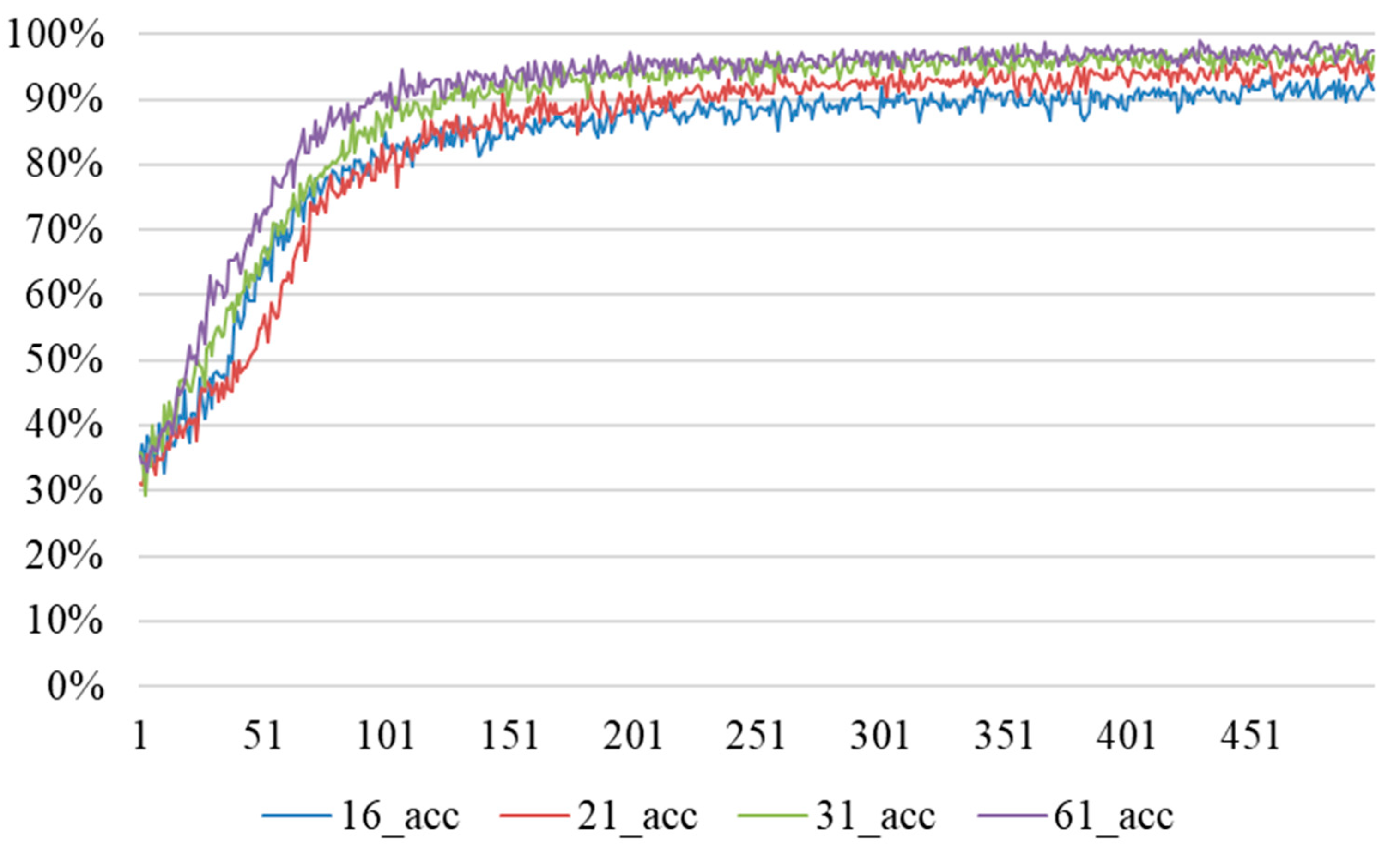
The resolution of the coffee granule image is adjusted to 3024 × 4032 so that tiny coffee granules can still be initially located. However, if the granules’ sizes are too small, they will be considered as small powders or noises and will be eliminated in the following morphological operations of the image processing. The coffee granule size distribution was first obtained through image processing, and then the size range was divided into 31 intervals. The granule counts of each size interval formed input vectors with only 31 elements to train the deep learning model. Therefore, the architecture of the workable deep learning model is not that complex. On the other hand, if coffee granule images are directly used as an input, the size of the input vector will be greatly increased; it will be very time-consuming to train a deep learning model with such a large input vector, and the resulting model will be considerably larger and much more complex than the proposed deep learning model in this paper.

Although morphological operations (erosion, dilation, opening, closing) caused propagation errors in coffee granule sizes, those propagation errors of coffee granule sizes can be reduced at the end of the image processing because the coffee granules are proportional to a reference coin with a known size and they were image processed together, suffering from the same causes of generating propagation errors. After computational analysis, the obtained low MSE (0.00399–15.22) and high PSNR (20.31–72.12 dB) values indicate the errors that are caused by morphological operations are small or acceptable. Therefore, those morphological operations mainly remove noise and fill small holes on coffee granules and do not cause obvious size errors. Furthermore, as the input vector to the deep learning model is formed using the number of granules in each size interval, even if there are some small coffee granule size errors, those coffee granules may still fall into the correct size interval and may not change the number of granules in that size interval. In addition, the output of the deep learning model in this paper are probability distributions rather than deterministic values. For a well-trained deep learning model for classification, the predicted class has the largest corresponding output probability, which is usually greater than the sum of the probabilities of the remaining classes. Therefore, the deep learning model allows for a little input uncertainty caused by coffee granule size errors without affecting the prediction consistency. That is why the input vector may not be susceptible to small size errors in coffee granules in our application. However, if the applications need to obtain deterministic size values, such as the applications in [13,14,15,16,17,18,19,20], the simple scale calibration using a reference object of known size could not be accurate enough. One should use image acquisition systems with pixel to length scale calibration, ambient brightness control, and a fixed shooting distance.

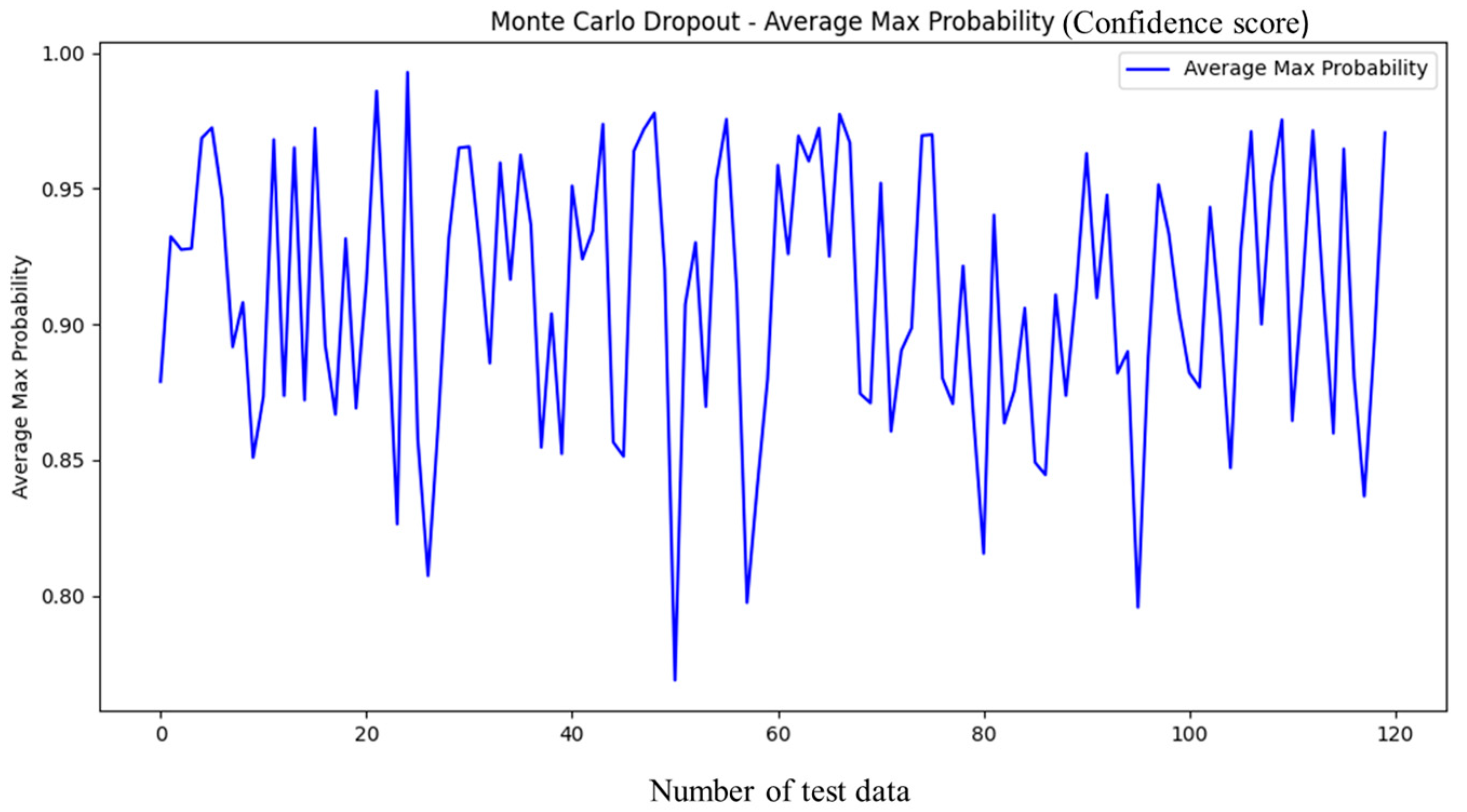
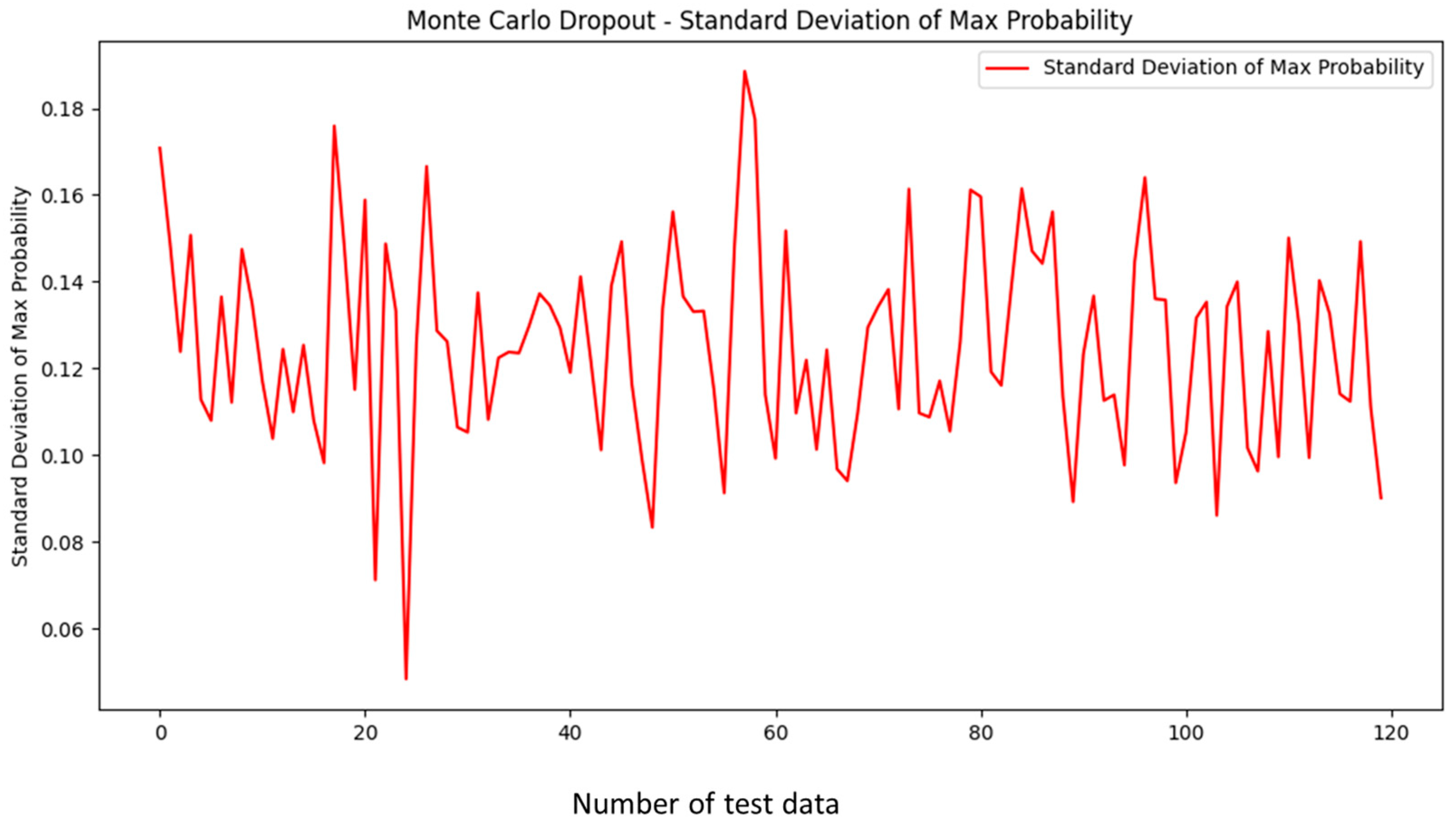
From the Monte Carlo dropout analysis for all 120 test data, the averages of max prediction probabilities (confidence scores, 0.75–0.99) are greater than 0.75, and all the standard deviations (uncertainties, 0.05–0.18) are below 0.2. Even considering the worst case, the max prediction probability is still above 0.55. Therefore, even if the selected deep learning model has uncertainties from dropout, it will not affect the consistency of prediction on the same test data in most cases. Consequently, the robustness of the selected deep learning model is assured.

Furthermore, the overall average of the prediction accuracy of 12,000 tests performed while running the above Monte Carlo dropout analysis is 96.67%. The effectiveness of the proposed method using a reference coin as a scale calibration, image processing, and the deep learning model are all successfully verified.

In experiments, the runtime for image processing is around 1 s while the runtime for burr wear level classification using the deep learning model is less than 0.5 s on a server computer. It only takes less than a minute for users to complete the LINE bot operation and receive the prediction with a long-term average accuracy of 96.67%. This accuracy is high enough for our application because coffee experts told us that when they performed their method twice using the same coffee granules, they had about a 2–3% chance of having inconsistent burr wear predictions.

To the best of the authors’ knowledge, we have not found another system with a similar concept and function for tool wear classification using the integration of a deep learning model and image processing on the granules produced by tools.

Compared with the prediction accuracies of indirect tool wear prediction applications using force signals, vibration signals, acoustic emission signals, current signals, and deep learning related models such as 94.2–99.8% in [29], 98.77–100% in [48], and 87.75% in [49], the accuracy of 96.67% for the method proposed in this paper is not inferior.

From the concepts of image acquisition and image data transfer and remote servers, an application to precisely measure particle size and shape in the Baijiu (Chinese liquor) brewing process using a smartphone-based imaging system [14] is similar to our system, but they need a specially built image acquisition platform with an accurate scale calibration of pixel to length. In that paper, without applying artificial intelligence, smartphones on a custom image acquisition platform can take photographs at a fixed distance using a custom designed APP to transfer the photos and communicate with the server and display the results. However, no design or operation details of that APP were provided. As the APP is custom designed, there is design overhead, and users need to use extra memory to install this APP on their smartphones and learn how to use it. In our system, we use the LINE bot to perform the same job, and no extra memory or user training are needed because LINE is already the dominant messaging APP on smartphones and almost everyone uses it daily in Taiwan. The morphological image processing for background extraction and noise removals in this paper is similar to ours. After that, their image processing departs from ours. They separate particles using a flood fill algorithm to label all pixels in the same connected components and then split the image into different connected areas and manually set upper and lower thresholds to only display the particles in the desired size range. Both the sizes and shapes of particles are obtained after further specialized calculations to obtain precise values.

5. Conclusions

To classify the coffee grinder burr wear level, instead of burr surface images obtained from costly scanning electron microscopes, coffee granule images taken by mobile phones are used for analysis. The analysis process running on a server computer is divided into two main steps. First, it applies image processing to obtain the coffee granule size distribution. Second, the input data with a unified length based on the coffee granule size distributions are used to train deep learning model with a compact structure and high accuracy. A chatbot interface using a LINE bot was built for remote users to conveniently send the coffee granule image, make requests to the server computer for analysis, and receive the burr wear level classification result.

In the performance-related analysis, low mean squared error (MSE, 0.00399–15.22) and high peak signal-to-noise ratio (PSNR, 20.31–72.12 dB) values indicate that the errors caused by morphological operations in image processing are small or acceptable. High confidence scores (0.75–0.99) and low standard deviations (0.05–0.18) from the Monte Carlo dropout analysis ensure the robustness of the prediction consistency of the deep learning model. With a prediction accuracy that is higher than 96%, the proposed design approach in both the image processing and deep learning model have been proven to be very effective.

The system has the advantages of low implementation cost, low operating cost, fast response speed, high accuracy, a user-friendly interface, and ease of use. Therefore, it is very suitable for both coffee chains and coffee lovers.

The proposed method of combining image processing, a deep learning model, and chatbot has potential to be further modified and applied to predict tool wear for machines that generate particles or debris and has wider applications in the future.

6. Patents

The authors plan to apply for patents in the near future.