Two-Step Relaxation of Non-Equilibrium Electrons in Graphene: The Key to Understanding Pump–Probe Experiments

Abstract

In the majority of experiments targeting nonlinear optical phenomena, the application of high-intensity pulses drives electrons in graphene into a strongly non-equilibrium state. Under these conditions, conventional perturbation theory falls short in explaining graphene’s intricate optical response because of significant deviations in electron distribution over energy states from the equilibrium Fermi-Dirac one. In this work, we present a two-step relaxation model capable of predicting the transient dynamics of graphene’s carriers out of equilibrium, from the generation of spectrally narrow populations of non-thermalized electrons and holes to the establishment of a hot-electron gas and its subsequent cooling toward equilibrium with the crystal lattice. By comparing our model calculations to experimental results, we demonstrate its reliability and relevance to pump–probe experiments, providing insights into the pivotal role of hot electrons in comprehending ultrafast dynamics in graphene.

1. Introduction

When two beams of light impinge on an optically nonlinear material simultaneously, under certain conditions, they interact in such a way that the energy is transferred from one beam to the other; this phenomenon is known as two-beam coupling [1]. Optical pump–probe spectroscopy is a technique for studying non-equilibrium electronic dynamics based on such a coupling of pump and probe beams, which finds applications across a range of fields, from physics and chemistry to materials science and biology [2]. This technique involves focusing a short pulse of a strong pump beam and, after a certain delay time, a weak probe beam on a sample to record the transmittance or reflectance of the probe light. By adjusting the delay between the pulses, one can study the transient evolution of the out-of-equilibrium electrons. In particular, different versions of the pump–probe technique have been widely used for studying the electronic response of graphene to fast optical excitations [3,4,5,6,7,8,9,10,11].

The nonlinear optical behavior of graphene has been a subject of intense debate ever since the initial theoretical prediction in 2007, suggesting that graphene could exhibit an exceptionally high nonlinear optical response in a broad spectral range [12]. By that time, graphene had already garnered recognition for its remarkable linear optical properties, attributed to its distinctive conical band structure. Demonstrating its nonlinear optical properties would further solidify its standing as an ideal material for optical applications with potential implications for advanced photonics and optoelectronics [13]. Since then, substantial and continuous efforts have been dedicated to the experimental characterization of graphene’s nonlinear properties. This includes the observation of higher harmonics [14,15,16], the Kerr effect [17,18], saturable absorption [19,20], and four wave-mixing [21,22], along with other nonlinear effects. While there may not be complete agreement on the measured quantities across different articles, the majority of them report high values for graphene’s nonlinear properties [23]. Theoretical investigations, particularly concerning the third-order nonlinearity, have taken diverse routes. Early approaches applied the Boltzmann equation to investigate the nonlinear optical response of graphene owing to intraband electronic transitions [12,24]. To incorporate interband contributions, researchers employed the Bloch equations solved using perturbation theory approximations, which allowed for the calculation of the third-order tensor of conductivity, ${\sigma }^{\left(3\right)}({\omega }_1,{\omega }_2,{\omega }_3)$ [25,26,27]. Although more intricate, this approach also allows for the calculation of even higher orders in the electric field. Additionally, since perturbation theory enables one to obtain explicit expressions for the conductivity tensor, it facilitates the exploration of all possible effects arising from the third-harmonic generation, difference frequency, and saturable absorption.

However, a fundamental problem arises with this approach: perturbation theory’s validity hinges on small field intensities. In practical nonlinear optics experiments, the intensities of the involved beams are very high, meaning that the theoretical description of the system goes far beyond the limits of perturbation theory. The electromagnetic fields applied to graphene are able to create populations of carriers that cannot be described assuming equilibrium chemical potentials (${\mu }_0$) and temperature ($T_0$) for the carriers throughout the calculations, as is the case of the perturbative approaches mentioned above. This seems to be unjustified for typical conditions of nonlinear optical experiments on graphene.

In recent experiments, Hafez et al. employed high-power THz pulses and showcased graphene’s remarkable proficiency in generating higher-order THz harmonics by shining THz radiation onto graphene under normal incidence [28]. They successfully detected signals up to the seventh order in single-layer graphene that were driven by electric fields reaching tens of kilovolts per centimeter, with very high conversion efficiencies. The field intensities were well beyond the range of validity of the perturbation theory used to describe the third-order nonlinearity owing to intraband electronic transitions [24]. The generation of such terahertz high-harmonics was probably made possible by the creation of hot Dirac fermions that oscillate at these new frequencies. Therefore, the explanation, in this case, does not rely solely on the conventional nonlinear theory but rather is a combination of coherent nonlinear effects with the generation and dynamics of hot electrons, resulting in a strongly nonlinear intraband THz conductivity. Furthermore, it is possible that the broad dispersion of experimental data for the third-order susceptibility (${\chi }^{\left(3\right)}$) in graphene, measured through the Kerr effect [23], is partially due to hot electrons generated in those experiments.

It is well known that monolayer graphene possesses inversion symmetry, which means that, under normal incidence, even-order nonlinear effects vanish. However, this symmetry can be broken by using oblique incidence. In a work published by Constant et al. [7,29], two femtosecond pulses in a pump–probe scheme with different incident angles were used to excite graphene surface plasmons (GSPs). The differential reflectance of the probe beam was then measured, yielding two types of signals: one non-resonant, present for any combination of incident angles, and the other that resonantly depended on the angles (for a given frequency difference between the pump and probe). In the latter case, the two oblique pulses, through phase-matching, were able to excite GSPs. One interesting observation from the results of Refs. [7,29] is that the predicted order of magnitude using the conventional theory for ${\chi }^{\left(2\right)}$ is three orders of magnitude smaller than what is needed to explain the experimental results [30,31]. This suggests, once again, that the usual perturbative nonlinear approach is not suitable for their description or, at least, that some further effects, such as strong deviations of the electronic system from thermal equilibrium, are to be taken into account.

“Hot carriers” is the term used to describe such out-of-equilibrium situations that typically arise in semiconductors subjected to high-intensity steady or optical fields, and the charge carriers rapidly acquire more energy than they would have in equilibrium with the crystal lattice. If the energy gain rate is higher than the rate at which they lose energy to the lattice, the carriers enter a quasi-equilibrium state with each other, with a much higher temperature than that of the lattice. Because of this high temperature, these carriers are commonly referred to as “hot” [32,33]. Their importance has been demonstrated for semiconductors [32,33] and metals [34,35]. In graphene, owing to its particular linear band structure and, consequently, low density of states around the Dirac points, this phenomenon is extremely relevant and fundamental to understanding the ultrafast dynamics of photoexcited carriers. Because of its short carrier–carrier scattering characteristic time, graphene rapidly creates a population of hot electrons in the conduction band and holes in the valence band that can be described by two Fermi–Dirac distributions with different Fermi levels but a common temperature [36,37]. Unlike assumed in the perturbative approach, where the Fermi level and temperature remain fixed at their equilibrium values, for hot electrons, these parameters are replaced by quasi-Fermi levels and an effective temperature, which are dynamic and depending on the intensity, the duration of the optical pulses, and other influencing factors. This situation is typical of pump–probe spectroscopy experiments. Several experimental works on graphene have been published, and all of them seem to indicate the presence of a population of hot carriers under strong optical excitation [3,4,5,6,7,8,9,10,11,38,39,40,41,42]. In this work, we formulate a two-step relaxation model designed to help in understanding the dynamic characteristics of out-of-equilibrium carriers. While previous models targeting this goal have been published [3,10,36,37,43], ours differs from them in several features, (such as the distinction between non-thermalized and hot carriers and spatial diffusion of the latter) that enable us to explore the temporal evolution of hot carriers and their responses to various experimental parameters in this non-equilibrium state. We emphasize that the relaxation of the excited electrons occurs in two steps: (i) fast thermalization and (ii) slower cooling. Both steps are taken into consideration explicitly in our model via corresponding balance equations (while, e.g., Ref. [37] considers only one balance equation for the whole concentration of all non-equilibrium electrons and the model of Ref. [10] includes only energy balance equations for the cooling stage). In order to test the reliability of our model, we compare it to experimental results obtained in pump–probe experiments by Constant et al. [7]. Our goal extends beyond the development of a hot electron dynamics model itself; we also present expressions for observables relevant in the framework of pump-probe spectroscopy. This not only elucidates the fundamental role that these electrons play but also facilitates a comprehensive understanding of pump–probe experiments and the operation of devices such as graphene-based photodetectors.

The article is organized as follows. In Section 2.1, we provide an overview of the dynamics that occur in graphene upon ultrafast optical excitation. This includes the generation of a hot carrier gas and the subsequent relaxation through various decay channels. In Section 2.2, we present a detailed description of our model, which enables us to calculate the transient evolution of both non-thermalized and thermalized carriers, and we delve into its impact on graphene’s optical conductivity and the distribution function of its electrons. In Section 3, we employ our hot electron model in order to reproduce and understand experimental differential reflectivity signals obtained by Constant et al. [7]. The final section is dedicated to a summary and concluding remarks.

2. Materials and Methods

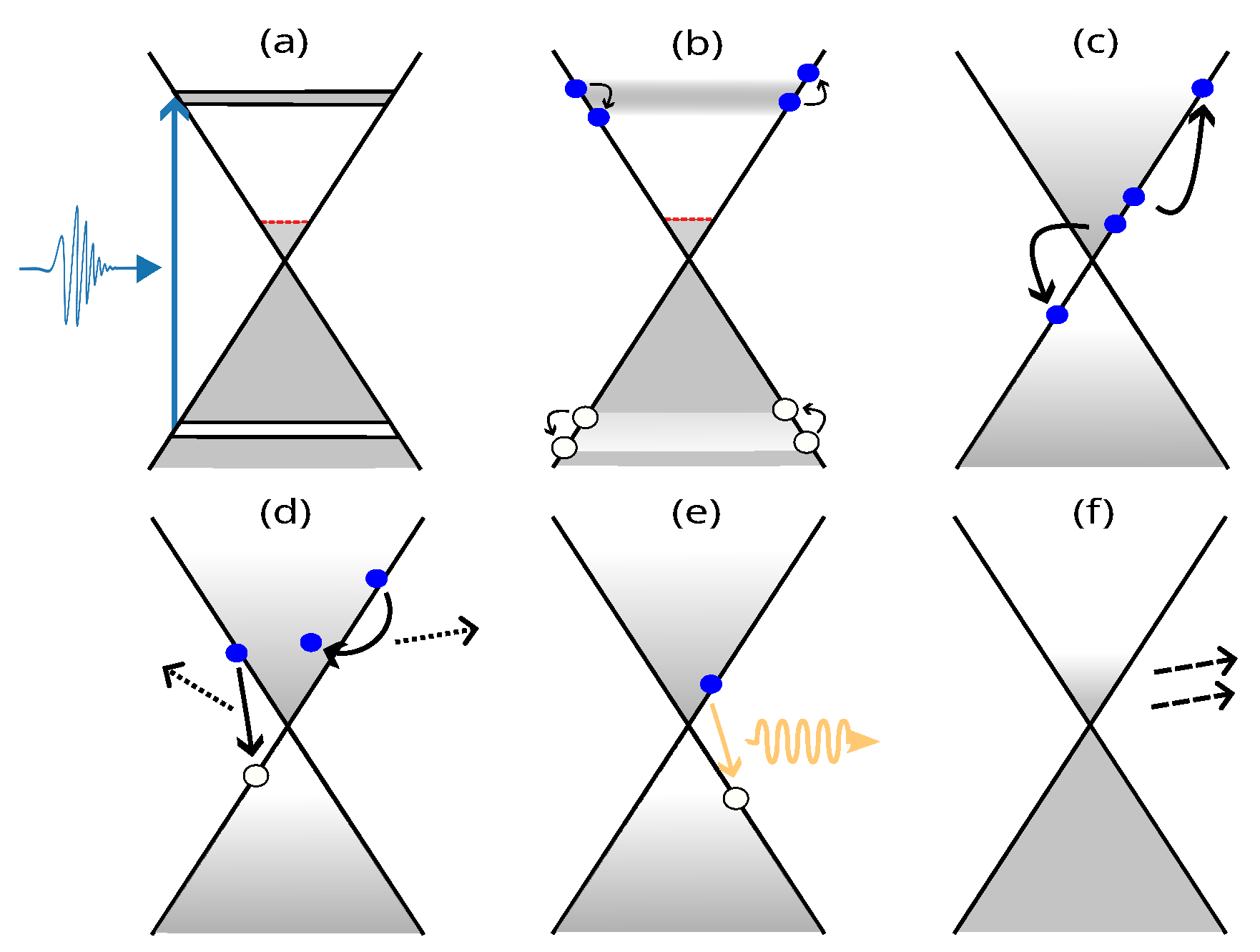
2.1. Carrier Dynamics in Graphene upon Ultrafast Optical Excitation

We start by discussing the ultrafast dynamics of non-equilibrium electrons in graphene [44], specifically when hot carriers are excited optically with an ultrafast laser pulse, typically in the femtosecond domain. We focus on interband excitation, when the incident pump photon energy $\hslash {\omega }_b$ is high enough to promote electrons to the conduction band, that is, when $\hslash {\omega }_b>2E_F$, with $E_F$ being the Fermi energy. When such an ultrafast laser pulse impinges on graphene, electrons from the valence band are excited to the conduction band. Therefore, two populations of non-thermalized particles are created: the excited electrons in the conduction band and the corresponding holes in the valence band. These non-thermalized carriers can hinder the transfer of additional electrons to the conduction band, and they evolve over time into separate thermal distributions, each characterized by its own temperature. The true equilibrium of such hot carriers is ultimately attained at a later stage when the excess energy is released to the lattice and the additional carriers created by light recombine.

The dynamics of these hot carriers in graphene is nowadays understood to occur via several stages and decay channels [44] (see Figure 1). Initially, the promptly excited carriers characterized by a spectrally narrow distribution primarily undergo carrier–carrier scattering on a 10 fs timescale [4,9], and two populations of hot carriers, one of electrons and another of holes, are formed. These populations can be described as Fermi-like distributions, featuring different chemical potentials while sharing a common temperature, distinct from that of the lattice [37]. Over longer timescales, the relaxation of hot carriers toward their equilibrium state is accomplished via several stages and decay channels, such as optical phonon emission [41], Auger recombination, and hot plasmon emission [45,46,47], on a timescale of hundreds of femtoseconds, as well as direct and disorder-assisted acoustic phonon emission on picoseconds scale. Thermalization with the lattice is achieved before the electron populations in both conduction and valence bands reach their equilibrium values (i.e., the electrons’ and holes’ quasi-Fermi levels become equal ($F_e=F_h=E_F$)). The recovery of the equilibrium concentrations of electrons and holes is the slowest process in graphene.

2.2. Electron Relaxation Model

In this section, we present our model for hot carriers in order to explain the dynamics of the electronic response of optically excited graphene. The goal is to determine the dynamics of the transient electron temperature and quasi-Fermi levels of the hot carriers and, finally, graphene’s optical conductivity in terms of appropriate parameters, such as characteristic relaxation times.

Let us consider a pump beam consisting of photons with energy $\hslash {\omega }_b$, inducing a non-thermalized population of electrons (holes) in the conduction (valence) band. The beam is focused on a circular spot on the graphene surface, where photocarriers are generated. We break down the hot carrier dynamics into two stages. The first stage spans the first few tens of fs with carrier–carrier collisions, which is faster than the pump duration (${\tau }_b\approx 100$ fs) and drives the system toward a quasi-equilibrium distribution, where the charge carriers have a very high temperature compared to that of the lattice. The second stage, on the scale of a few hundred fs, occurs when the relaxation of carrier energy and electron–hole recombination take place. To model these processes, we introduce three adjustable parameters:

• Electron–electron (as well as hole–hole and electron–hole) scattering time, ${\tau }_{ee}$;
• Energy intraband relaxation time, ${\tau }_{\epsilon }$, due to the electron scattering by lattice phonons, which is of the order of picoseconds, slightly exceeding the momentum relaxation time;
• Interband recombination time, ${\tau }_r$, determined by Auger recombination or via optical phonon or plasmon emission.

These parameters satisfy the following relation [37]:

$${\tau }_{ee}\ll {\tau }_{\epsilon }\ll {\tau }_r.$$

(1)

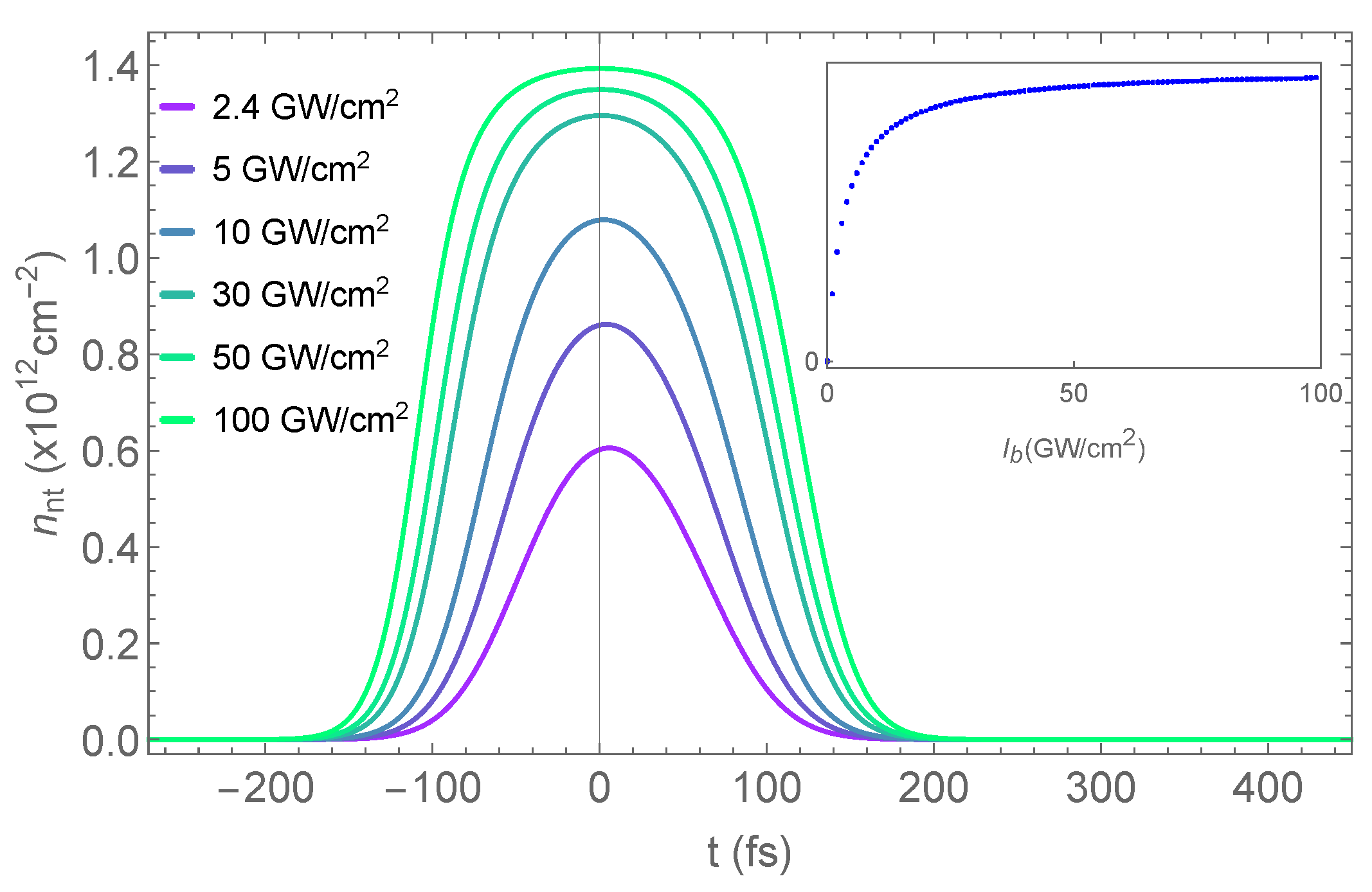
2.2.1. Non-Thermalized Carriers

We start by writing down equations that describe the populations of non-thermalized electrons, $n_{\mathrm{nt}}$, and holes, $p_{\mathrm{nt}}$, in optically excited graphene. Given the symmetry of their spectra (within the Dirac cone approximation) and the unique scattering time, ${\tau }_{ee}$, both electrons and holes evolve in the same way, so the non-thermalized populations are equal:

$$p_{\mathrm{nt}}(\overrightarrow{r},t)=n_{\mathrm{nt}}(\overrightarrow{r},t).$$

(2)

Owing to the carrier–carrier scattering, two populations of thermalized (i.e., having reached equilibrium among them but not with the environment) carriers are created. We denote the 2D concentration of the thermalized (hot) electrons by $n_{\mathrm{t}}(\overrightarrow{r},t)$ and the thermalized holes by $p_{\mathrm{t}}(\overrightarrow{r},t)$. Therefore, the total concentrations of electrons and holes are expressed as

$$n(\overrightarrow{r},t)=n_{\mathrm{nt}}(\overrightarrow{r},t)+n_{\mathrm{t}}(\overrightarrow{r},t);$$

(3)

$$p(\overrightarrow{r},t)=p_{\mathrm{nt}}(\overrightarrow{r},t)+p_{\mathrm{t}}(\overrightarrow{r},t).$$

(4)

The balance equations governing the depletion of carriers from the non-thermalized to the thermalized population are

$${\dot{p}}_{\mathrm{nt}}(\overrightarrow{r},t)={\dot{n}}_{\mathrm{nt}}(\overrightarrow{r},t)={\displaystyle \frac{A(\overrightarrow{r},t)}{\hslash {\omega }_b}}{I}_b(\overrightarrow{r},t)-{\displaystyle \frac{n_{\mathrm{nt}}(\overrightarrow{r},t)}{{\tau }_{ee}}},$$

(5)

where

$$I_b(\overrightarrow{r},t)=I_b^{\max }exp\left(-{\displaystyle \frac{2t^2}{{\tau }_b^2}}\right)exp\left(-{\displaystyle \frac{\ln 2}{w_0^2}}{r}^2\right)$$

(6)

is the pump intensity, $I_b^{\max }$ is the peak intensity value, $w_0$ is the effective radius of the pump beam, and

$$A(\overrightarrow{r},t)=A_0(\alpha ,\theta )\left\{1-g_h\left(-{\displaystyle \frac{\hslash {\omega }_b}{2}},\overrightarrow{r},t\right)-g_e\left({\displaystyle \frac{\hslash {\omega }_b}{2}},\overrightarrow{r},t\right)\right\}$$

(7)

is the time-dependent absorbance of graphene (see Section S1 of the Supplementary Material for details). Here, $g_e$ and $g_h$ are the non-thermalized distribution functions for electrons and holes, respectively, and

$$A_0(\alpha ,\theta )={\displaystyle \frac{4\pi {\alpha }_F}{{\left(ncos\alpha +cos\theta \right)}^2}}cos\alpha {cos}^2\theta$$

(8)

is the absorbance amplitude, with $\alpha$ and $\theta$ denoting the incident and refraction angles of the pump beam (with respect to the normal to the surface) and n denoting the refractive index of the substrate. Equation (8) holds for transverse magnetic (TM) polarization. Note that the first term in Equation (5) corresponds to the generation of non-thermalized carriers and the second one to their thermalization.

According to Equation (2), the non-thermalized distributions $g_e$ and $g_h$ in Equation (7) should be equal:

$$g_h(-\epsilon ,\overrightarrow{r},t)=g_e(\epsilon ,\overrightarrow{r},t)=g(\epsilon ,\overrightarrow{r},t).$$

(9)

Since the pump pulse is described by a Gaussian wavepacket in the frequency domain, $g(\epsilon ,\overrightarrow{r},t)$ is modeled as

$$g(\epsilon ,\overrightarrow{r},t)=\tilde{g}(\overrightarrow{r},t){\displaystyle \frac{{\Delta }_{\epsilon }(-\infty )}{{\Delta }_{\epsilon }\left(t\right)}}exp\left(-{\displaystyle \frac{{\left(\epsilon -\hslash {\omega }_b/2\right)}^2}{2{\Delta }_{\epsilon }^2\left(t\right)}}\right),$$

(10)

where $\tilde{g}(\overrightarrow{r},t)$ can be expressed in terms of the non-thermalized population of charge carriers:

$$\tilde{g}(\overrightarrow{r},t)={\displaystyle \frac{n_{\mathrm{nt}}(\overrightarrow{r},t)}{2n_{\mathrm{nt}}^{\max }}}.$$

(11)

Here, $n_{\mathrm{nt}}^{\max }=\sqrt{\frac{\pi }{2}}{\Delta }_{\epsilon }\rho \left({\displaystyle \frac{\hslash {\omega }_b}{2}}\right)$ is the maximum possible concentration of non-thermalized electrons (holes) (the factor of 1/2 in Equation (11) appears because the absorption vanishes for $g(\epsilon ,\overrightarrow{r},t)=\frac{1}{2}$; see Equations (7) and (9)). These expressions are derived in Section S2 of the Supplementary Material.

In order to proceed, we make the following simplifying assumptions:

• Since the pulse is much longer in time than ${\tau }_{ee}$, during pumping, a stationary situation is rapidly achieved for the distribution width ${\Delta }_{\epsilon }\left(t\right)$, so we take its asymptotic limit: ${\Delta }_{\epsilon }\left(t\right)\approx {\Delta }_{\epsilon }(-\infty )$;
• For 100 fs pulses, their spectral width ($\sim$8 meV) should be much smaller than the thermalized distribution energy spread, so we take ${\Delta }_{\epsilon }(-\infty )$ to be the Gaussian pulse’s spectral width:

  $${\Delta }_{\epsilon }(-\infty )={\displaystyle \frac{\hslash }{{\tau }_b}}=\sqrt{2\ln 2}\frac{\hslash }{\Delta t},$$

  (12)

  where $\Delta t$ is the full width at half-maximum (FWHM) of the pulse in the time domain.
• As the thermalized carriers relax toward lower energies, we assume that their distributions, $f_e$ and $f_h$, for $\epsilon \approx \hslash {\omega }_b/2$, are such that

  $$f_e\left(\epsilon ,\overrightarrow{r},t\right)\ll g_e(\epsilon ,\overrightarrow{r},t),$$

  (13)

  $$f_h\left(\epsilon ,\overrightarrow{r},t\right)\ll g_h(\epsilon ,\overrightarrow{r},t),$$

  (14)

  so they do not affect the pump photon’s absorption.

With these assumptions, Equation (5) is simplified to

$${\dot{n}}_{\mathrm{nt}}(\overrightarrow{r},t)={\displaystyle \frac{A_0(\alpha ,\theta )}{\hslash {\omega }_b}}{I}_b(\overrightarrow{r},t)\left\{1-{\displaystyle \frac{n_{\mathrm{nt}}(\overrightarrow{r},t)}{n_{\mathrm{nt}}^{\max }}}\right\}-{\displaystyle \frac{n_{\mathrm{nt}}(\overrightarrow{r},t)}{{\tau }_{ee}}}.$$

(15)

The temporal evolution of $n_{\mathrm{nt}}$ in the center of the pump spot is illustrated in Figure 2 for different intensities of the pump beam. As expected, this concentration rises with the increase in pump beam intensity. Nonetheless, as indicated in the inset, this value starts to saturate at higher intensities, ultimately attaining its maximum value ($n_{\mathrm{nt}}^{\max }$), indicating saturable absorption. Furthermore, it can be seen that, at lower intensities, the peak shifts toward later times in comparison to higher intensities. This phenomenon arises because of the balance between non-thermalized electrons, excited by the pump beam, and electrons undergoing thermalization over a timescale of ${\tau }_{ee}$. At lower intensities, electrons are promoted to the conduction band, but they remain non-thermalized within the timescale of ${\tau }_{ee}$ until they become thermalized. This accounts for the observed shift in the peak compared to $t=0$. In contrast, at higher pump intensities, the substantial influx of promoted electrons leads to the peak occurring at $t=0$, yet the concentration of non-thermalized electrons remains stable for a few femtoseconds.

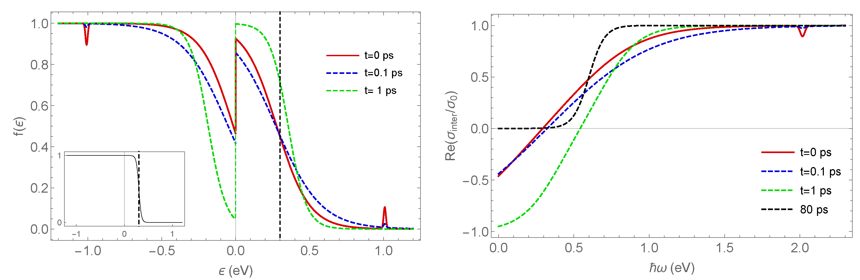
2.2.2. Thermalized Carriers

After the creation of the non-thermalized population, $n_{\mathrm{nt}}+p_{\mathrm{nt}}$, photocarriers undergo electron–electron, electron–hole, and hole–hole scattering processes leading to a quasi-equilibrium of the (hot) electron and hole gases. The electron and hole distributions are approximated by quasi-Fermi–Dirac functions with transient chemical potentials (quasi-Fermi levels) $F_e$ and $F_h$, respectively, and a unique electronic temperature T:

$$f_e(\epsilon ,F_e,T)=f_c\left(\epsilon \right)={\displaystyle \frac{1}{1+exp\left({\displaystyle \frac{\epsilon -F_e}{k_{B}T}}\right)}},\epsilon >0;$$

(16)

$$f_h(\epsilon ,F_h,T)=1-f_v\left(\epsilon \right)={\displaystyle \frac{1}{1+exp\left({\displaystyle \frac{F_h-\epsilon }{k_{B}T}}\right)}},\epsilon <0.$$

(17)

This assumption is justified if the electron–electron, electron–hole, and hole–hole scattering processes (characterized by the typical scattering time ${\tau }_{ee}$) are more probable than the electron–phonon and electron–impurity ones. Experimental results [4,5] indicate that this situation is usually the case in typical graphene samples. The distribution functions (16) and (17) are considered slowly varying functions of time on the scale $t\gg {\tau }_{ee}$. In principle, they are also functions of $\overrightarrow{r}$, but we apply an averaging procedure explained below in order to avoid complications with local (spatially-dependent) chemical potentials and temperature.

To model the evolution of thermalized carriers, we write down balance equations for $n_t$ and $p_t$ as

$${\dot{n}}_{\mathrm{t}}(\overrightarrow{r},t)={\displaystyle \frac{n_{\mathrm{nt}}(\overrightarrow{r},t)}{{\tau }_{ee}}}+D{\nabla }^2{n}_{\mathrm{t}}(\overrightarrow{r},t)-{\displaystyle \frac{n_t(\overrightarrow{r},t)-n_0}{{\tau }_r}};$$

(18)

$${\dot{p}}_{\mathrm{t}}(\overrightarrow{r},t)={\displaystyle \frac{p_{\mathrm{nt}}(\overrightarrow{r},t)}{{\tau }_{ee}}}+D{\nabla }^2{p}_{\mathrm{t}}(\overrightarrow{r},t)-{\displaystyle \frac{p_t(\overrightarrow{r},t)-p_0}{{\tau }_r}}.$$

(19)

Equations (18) and (19) include a diffusion term ($D{\nabla }^2$) to take into account the departure of thermalized carriers from the pump spot. The importance of diffusion of hot carriers for a very sharp spatial profile of excitation has been shown experimentally [40].

At a timescale of ∼${\tau }_{\epsilon }$, the thermalized electrons, scattered mostly by phonons, give their energy, ${\epsilon }_t$, to the lattice, and the electron energy relaxation is described by the following balance equation:

$${\dot{\epsilon }}_t(\overrightarrow{r},t)={\displaystyle \frac{{\epsilon }_{\mathrm{nt}}(\overrightarrow{r},t)}{{\tau }_{ee}}}+D_{\epsilon }{\nabla }^2{\epsilon }_{\mathrm{t}}(\overrightarrow{r},t)-{\displaystyle \frac{{\epsilon }_t(\overrightarrow{r},t)-{\epsilon }_0^{\prime }\left(t\right)}{{\tau }_{\epsilon }}},$$

(20)

where ${\epsilon }_0^{\prime }$ is the energy density at the equilibrium temperature but with a chemical potential out of equilibrium, reflecting the rapid decay of temperature compared to the quasi-Fermi levels. In (20), $D_{\epsilon }$ denotes the thermal diffusivity, which can be related to the diffusion coefficient; actually, with a good approximation, $D_{\epsilon }\approx D$, as demonstrated in Section S3 of the Supplementary Material.

The energy of the non-thermalized electrons, ${\epsilon }_{\mathrm{nt}}$, can be defined as

$$\begin{array}{cc}\hfill {\epsilon }_{\mathrm{nt}}(\overrightarrow{r},t)& ={\int }_0^{+\infty }d\epsilon \epsilon \rho \left(\epsilon \right)g(\epsilon ,\overrightarrow{r},t)\hfill \\ \hfill & =exp\left(-{\displaystyle \frac{{\hslash }^2{\omega }_b^2}{8{\Delta }_E^2}}\right)\rho \left({\displaystyle \frac{\hslash {\omega }_b}{2}}\right){\Delta }_{\epsilon }^2\tilde{g}(\overrightarrow{r},t)+\sqrt{2\pi }{\Delta }_{\epsilon }\rho \left({\displaystyle \frac{\hslash {\omega }_b}{2}}\right)\left[{\displaystyle \frac{\hslash {\omega }_b}{2}}+{\displaystyle \frac{2{\Delta }_{\epsilon }^2}{\hslash {\omega }_b}}\right]\tilde{g}(\overrightarrow{r},t).\hfill \end{array}$$

(21)

Since $2{\Delta }_{\epsilon }\ll \hslash {\omega }_b$, by employing Equation (11), ${\epsilon }_{\mathrm{nt}}$ approximates to

$${\epsilon }_{\mathrm{nt}}(\overrightarrow{r},t)\approx {\displaystyle \frac{\hslash {\omega }_b}{2}}{n}_{\mathrm{nt}}(\overrightarrow{r},t),$$

(22)

and Equation (20) can be simplified:

$${\dot{\epsilon }}_t(\overrightarrow{r},t)\approx {\displaystyle \frac{\hslash {\omega }_b}{2}}{\displaystyle \frac{n_{\mathrm{nt}}(\overrightarrow{r},t)}{{\tau }_{ee}}}+D_{\epsilon }{\nabla }^2{\epsilon }_{\mathrm{t}}(\overrightarrow{r},t)-{\displaystyle \frac{{\epsilon }_t(\overrightarrow{r},t)-{\epsilon }_0^{\prime }\left(t\right)}{{\tau }_{\epsilon }}}.$$

(23)

In typical optical experiments, it is usual to take a spatial average over the measured signal in the detector. With this in mind, in order to avoid the spatial dependence of $F_e$, $F_h$, and T, we substitute the functions $n_{nt}(\overrightarrow{r},t)$, $n_t(\overrightarrow{r},t)$, $p_t(\overrightarrow{r},t)$, and ${\epsilon }_t(\overrightarrow{r},t)$ by their spatial average values. This averaging procedure is carried out using a weight function defined as

$$f\left(\overrightarrow{r}\right)={\displaystyle \frac{\ln 2}{\pi w_0^2}}exp\left[-{\displaystyle \frac{\ln 2}{w_0^2}}{\left(\overrightarrow{r}-{\overrightarrow{r}}_0\right)}^2\right].$$

(24)

The reason for choosing this form for the weight function becomes clear in Section 3. Notice that it is normalized to unity if ${\overrightarrow{r}}_0=0$ (pumping into the center of the detection area).

Using Green’s function for the diffusion equation, we obtain a semi-analytical solution for Equations (18) and (23) without applying any approximation (see Section S4 of the Supplementary Material), and the resulting expressions are

$$\begin{array}{cc}\hfill n_{\mathrm{t}}\left(t\right)\equiv \langle n_{\mathrm{t}}(t,\overrightarrow{r})\rangle & =n_0+\tilde{n}\left(t\right);\hfill \end{array}$$

(25)

$$\begin{array}{cc}\hfill {\epsilon }_{\mathrm{t}}\left(t\right)\equiv \langle {\epsilon }_{\mathrm{t}}(t,\overrightarrow{r})\rangle & ={\epsilon }_0^{\prime }\left(t\right)+\tilde{\epsilon }\left(t\right),\hfill \end{array}$$

(26)

where

$$\begin{array}{cc}\hfill \tilde{n}\left(t\right)& ={\displaystyle \frac{2\ln 2}{{\tau }_{\mathrm{ee}}}}{\int }_{-\infty }^{t}d{t}^{\prime }{\int }_0^{\infty }{r}^{\prime }d{r}^{\prime }{\displaystyle \frac{e^{-(t-t^{\prime })/{\tau }_r}{n}_{\mathrm{nt}}(r^{\prime },t^{\prime })}{w_0^2+4\ln 2D(t-t^{\prime })}}exp\left[-{\displaystyle \frac{\ln 2{(r^{\prime }-r_0)}^2}{w_0^2+4\ln 2D(t-t^{\prime })}}\right];\hfill \end{array}$$

(27)

$$\begin{array}{cc}\hfill \tilde{\epsilon }\left(t\right)& ={\displaystyle \frac{\ln 2\hslash {\omega }_b}{{\tau }_{\mathrm{ee}}}}{\int }_{-\infty }^{t}d{t}^{\prime }{\int }_0^{\infty }{r}^{\prime }d{r}^{\prime }{\displaystyle \frac{e^{-(t-t^{\prime })/{\tau }_{\epsilon }}{n}_{\mathrm{nt}}(r^{\prime },t^{\prime })}{w_0^2+4\ln 2D_{\epsilon }(t-t^{\prime })}}exp\left[-{\displaystyle \frac{\ln 2{(r^{\prime }-r_0)}^2}{w_0^2+4\ln 2D_{\epsilon }(t-t^{\prime })}}\right].\hfill \end{array}$$

(28)

Note that the spatial average has already been performed.

On the other hand, the instantaneous thermalized electron concentration and energy density can be related to the quasi-Fermi level $F_e\left(t\right)$ and the electronic temperature $T\left(t\right)$ as

$$\begin{array}{cc}\hfill n_t\left(t\right)& ={\displaystyle \frac{g_s{g}_v}{\mathcal{S}}}\sum _{\mathrm{k}}{f}_e\left({\epsilon }_{\mathrm{k}},F_e\left(t\right),T\left(t\right)\right)={\displaystyle \frac{2}{\pi }}{\left({\displaystyle \frac{k_{B}T\left(t\right)}{\hslash v_F}}\right)}^2\mathrm{\Gamma }\left(2\right){\mathrm{F}}_1\left({\displaystyle \frac{F_e\left(t\right)}{k_{B}T\left(t\right)}}\right);\hfill \end{array}$$

(29)

$$\begin{array}{cc}\hfill {\epsilon }_t\left(t\right)& ={\displaystyle \frac{g_s{g}_v}{\mathcal{S}}}\sum _{\mathrm{k}}{\epsilon }_{\mathrm{k}}{f}_e\left({\epsilon }_{\mathrm{k}},F_e\left(t\right),T\left(t\right)\right)={\displaystyle \frac{2}{\pi }}{\displaystyle \frac{{\left(k_{B}T\left(t\right)\right)}^3}{{\left(\hslash v_F\right)}^2}}\mathrm{\Gamma }\left(3\right)F_2\left({\displaystyle \frac{F_e\left(t\right)}{k_{B}T\left(t\right)}}\right),\hfill \end{array}$$

(30)

where $g_s$ and $g_v$ are the spin and valley degeneracies for graphene, respectively, and ${\mathrm{F}}_n\left(z\right)$ is the Fermi integral:

$${\mathrm{F}}_n\left(z\right)={\displaystyle \frac{1}{\mathrm{\Gamma }(n+1)}}{\int }_0^{+\infty }dx{\displaystyle \frac{x^n}{1+exp\left(x-z\right)}}$$

(31)

with $\mathrm{\Gamma }\left(n\right)$ being the Euler gamma function. With these expressions, it is also clear how to evaluate $n_0$ and ${\epsilon }_0^{\prime }\left(t\right)$.

Thus, using Equations (25), (26), (29), and (30), we can define the following system of equations:

$$\begin{array}{cc}\hfill n_0+\tilde{n}\left(t\right)& ={\displaystyle \frac{2}{\pi }}{\left({\displaystyle \frac{k_{B}T\left(t\right)}{\hslash v_F}}\right)}^2\mathrm{\Gamma }\left(2\right){\mathrm{F}}_1\left({\displaystyle \frac{F_e\left(t\right)}{k_{B}T\left(t\right)}}\right);\hfill \end{array}$$

(32)

$$\begin{array}{cc}\hfill {\epsilon }_0^{\prime }\left(t\right)+\tilde{\epsilon }\left(t\right)& ={\displaystyle \frac{2}{\pi }}{\displaystyle \frac{{\left(k_{B}T\left(t\right)\right)}^3}{{\left(\hslash v_F\right)}^2}}\mathrm{\Gamma }\left(3\right)F_2\left({\displaystyle \frac{F_e\left(t\right)}{k_{B}T\left(t\right)}}\right),\hfill \end{array}$$

(33)

enabling us to determine the transient evolution of $F_e\left(t\right)$ and $T\left(t\right)$. Yet, it remains to determine the holes’ chemical potential. By virtue of the local charge neutrality, we can simply define a third equation as

$$p_0+n\left(t\right)=p\left(t\right)+n_0,$$

(34)

which means that we can also compute the transient evolution of the holes’ chemical potential.

After getting excited, the non-thermalized carriers undergo electron–electron scattering events. Theoretical work [48] and experimental evidence [4] indicate that these scattering processes are much more probable in the first few femtoseconds than the electron–phonon ones. As a result, the distribution of the non-thermalized carriers is broadened and, owing to the bottleneck shape of the Dirac cone, evolves toward a Fermi-like distribution [5] much faster than the carriers can lose energy to the lattice. This idea is expressed through Equations (20) and (22): the energy of the non-thermalized electrons, ${\epsilon }_{\mathrm{nt}}$, is transferred to the thermalized carriers essentially at the same rate as their population, $n_{\mathrm{nt}}$, namely, $1/{\tau }_{\mathrm{ee}}$. In fact, as a consequence of Equation (22), ${\epsilon }_{\mathrm{nt}}$ obeys a balance equation in the same form as Equation (15) for $n_{\mathrm{nt}}$. Thus, in our model, only the thermalized (hot) carriers transfer energy to the lattice.

2.2.3. Low Pump Intensity Approximation

The system of Equations (32)–(34) has to be solved numerically, and the computation of the transient evolution of $F_e$, $F_h$, and T is rather time-consuming, mostly because of the spatial integration in Equations (27) and (28). To address this issue, we can employ an approximation. Since Equation (15) is nonlinear, separating the spatial and temporal components in the equation is not possible. However, if the pump intensities used are not too high so that the term $n_{\mathrm{nt}}/n_{\mathrm{nt}}^{\max }$ is small, we can assume that the spatial distribution is minimally affected in the initial tens of femtoseconds. Under this assumption, the concentration of non-thermalized carriers can approximately be expressed as

$$n_{\mathrm{nt}}(\overrightarrow{r},t)\approx exp\left(-{\displaystyle \frac{\ln 2}{w_0^2}}{r}^2\right){\overline{n}}_{\mathrm{nt}}\left(t\right),$$

(35)

where ${\overline{n}}_{\mathrm{nt}}$ is the solution of Equation (15) neglecting the spatial part. Therefore, the spatial integrals in Equations (27) and (28) can be solved analytically and one obtains

$$\begin{array}{cc}\hfill n_t\left(t\right)& =n_0+{\displaystyle \frac{w_0^2}{{\tau }_{ee}}}{\int }_{-\infty }^t{\displaystyle \frac{e^{-(t-t^{\prime })/{\tau }_r}{\overline{n}}_{\mathrm{nt}}\left(t^{\prime }\right)}{\left(2w_0^2+4\ln \left(2\right)D(t-t^{\prime })\right)}}exp\left[-{\displaystyle \frac{\ln \left(2\right)r_0^2}{2w_0^2+4\ln \left(2\right)D(t-t^{\prime })}}\right]d{t}^{\prime };\hfill \end{array}$$

(36)

$$\begin{array}{cc}\hfill {\epsilon }_t\left(t\right)& ={\epsilon }_0^{\prime }\left(t\right)+{\displaystyle \frac{\hslash {\omega }_b}{2}}{\displaystyle \frac{w_0^2}{{\tau }_{ee}}}{\int }_{-\infty }^t{\displaystyle \frac{e^{-(t-t^{\prime })/{\tau }_{\epsilon }}{\overline{n}}_{\mathrm{nt}}\left(t^{\prime }\right)}{2w_0^2+4\ln \left(2\right)D_{\epsilon }(t-t^{\prime })}}exp\left[-{\displaystyle \frac{\ln \left(2\right)r_0^2}{2w_0^2+4\ln \left(2\right)D_{\epsilon }(t-t^{\prime })}}\right]d{t}^{\prime }.\hfill \end{array}$$

(37)

By employing these expressions, we can assess the transient evolution of the parameters of interest more efficiently. Figure 3 shows the variation of $F_e$, $F_h$, and T with time for different values of the pump spot radius (which determines the importance of the diffusion term in the balance equations). In the left panel, the solid (dashed) lines depict the variation of the quasi-Fermi level for electrons (holes), while the right panel illustrates the transient evolution of temperature. It is clear from the presented results that, for stronger focused beams, the diffusion effect is more pronounced and the transient evolution of the considered parameters is faster, as a larger number of electrons escape from the excitation spot and do not contribute to the spatial averages that determine the observable quantities, such as probe beam’s reflectivity.

2.2.4. Non-Equilibrium Conductivity Due to Hot Carriers

Given the quasi-Fermi levels and the electronic temperature as functions of t, we can introduce the transient optical conductivity. We assume that, to the first order, the interband conductivity of graphene can be described by the usual formula [49]:

$${\sigma }_{\mathrm{inter}}(\omega ,t)={\displaystyle \frac{4{\sigma }_0}{\pi }}\hslash \left({\gamma }_{\mathrm{inter}}-i\omega \right){\int }_0^{+\infty }d\epsilon {\displaystyle \frac{1-f^{\left(e\right)}(\epsilon ,t)-f^{\left(h\right)}(\epsilon ,t)}{\left[\hslash {\gamma }_{\mathrm{inter}}+i\left(2\epsilon -\hslash \omega \right)\right]\left[\hslash {\gamma }_{\mathrm{inter}}-i\left(2\epsilon +\hslash \omega \right)\right]}}$$

(38)

with ${\gamma }_{\mathrm{inter}}$ meaning the interband scattering rate. Here, $f^{\left(e\right)}$ and $f^{\left(h\right)}$ are the full distribution functions for the electrons and holes with contributions from thermalized and non-thermalized carriers:

$$f^{(e,h)}(\epsilon ,t)=g_{e,h}(\epsilon ,t)+f_{e,h}\left(\epsilon ,F_{e,h}\left(t\right)\right)$$

(39)

with $g_{e,h}$ given in Equation (9).

The extension of the usual formula for the interband conductivity to the time-dependent version (38), similar to the slowly varying amplitude approximation for optical pulses, is valid as long as the electric field oscillates (with the frequency $\omega$) several times before the physical conditions change. In other words, this approach works if the two timescales, $1/\omega$ and the time it takes for chemical potentials and temperature to change, are sufficiently different, and

$$\omega {\tau }_{\mathrm{ee}}\gg 1.$$

(40)

Here, we take ${\tau }_{ee}$ as the shortest characteristic time in the system. Since it is expected that ${\tau }_{ee}$ lies in the range of 10–30 fs [4], this condition is satisfied for optical frequencies.

As we see below, to the first order, the differential reflectivity depends only on the real part of the transient conductivity. Also, it is expected that $\hslash {\gamma }_{\mathrm{inter}}\ll k_{B}T$ [37], so the real part of the expression (38) can be written as

$$\mathrm{Re}{\sigma }_{\mathrm{inter}}(\omega ,t)=\mathrm{Re}{\sigma }_{\mathrm{nt}}(\omega ,t)+\mathrm{Re}{\sigma }_t(\omega ,t)$$

(41)

with ${\sigma }_t(\omega ,t)$ coming from the thermalized (hot) carriers,

$$\mathrm{Re}{\sigma }_t(\omega ,t)={\sigma }_0{\displaystyle \frac{sinh\left[{\displaystyle \frac{\hslash \omega -\left(F_e\left(t\right)-F_h\left(t\right)\right)}{2k_{B}T}}\right]}{cosh\left[{\displaystyle \frac{F_h\left(t\right)+F_e\left(t\right)}{2k_{B}T}}\right]+cosh\left[{\displaystyle \frac{\hslash \omega -\left(F_e\left(t\right)-F_h\left(t\right)\right)}{2k_{B}T}}\right]}},$$

(42)

and ${\sigma }_{\mathrm{nt}}(\omega ,t)$ from the non-thermalized ones [50],

$$\mathrm{Re}{\sigma }_{\mathrm{nt}}(\omega ,t)=-{\sigma }_{0}g\left({\displaystyle \frac{\hslash \omega }{2}},t\right).$$

(43)

Figure 4 presents the time evolution of both the hot-electron distribution function and the real part of the optical conductivity calculated using Equations (39) and (41), respectively. The distribution function begins in a state of equilibrium; however, after the carriers undergo thermalization, two Fermi-Dirac-like distributions emerge for electrons and holes, characterized by distinct quasi-Fermi levels and unique electronic temperatures. Both distribution functions exhibit a small peak corresponding to the non-thermalized carrier population, which can be seen for some time after the excitation. We notice that a discontinuity of the occupation probability (red line in Figure 4, left) arises at zero energy, an artifact due to our use of two distinct distributions to describe the carriers. However, it does not affect the optical conductivity. Despite this artifact, owing to the imposed form of the non-equilibrium distribution function, qualitatively, it resembles quite closely the one calculated in Ref. [48] via solving the Boltzmann equation (which is a much more time-consuming approach).

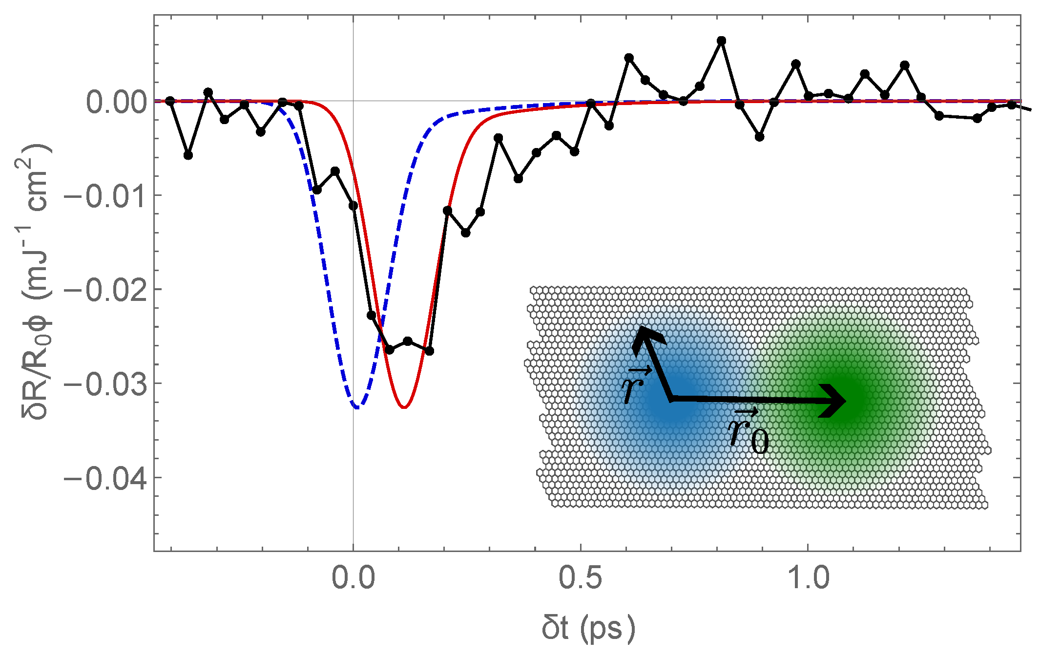
3. Case Study Results and Discussion

As mentioned in the introduction, our hot electron model can be used to understand and simulate the results acquired through pump–probe experiments, where the pump’s role is to excite a substantial concentration of photocarriers, which eventually form a population of hot electrons and holes. The latter then gradually dissipate their energy into the lattice via multiple decay pathways, as depicted in Figure 1. Due to their exceedingly high temperature, resulting in a very broad distribution over energies, the hot electrons can impede further transitions between the valence and conduction bands, with the absorption of probe beam photons, because of the Pauli blocking, both below and above the pump photon energy. Notably, because of the inverted electron population above $\epsilon =0$, the real part of the conductivity takes on negative values within a certain spectral range, implying an optical gain in this region [42]. The spectral width of this region is determined by the condition of population inversion, $f(\hslash \omega /2)>f(-\hslash \omega /2)$. It extends up to 0.6 eV for $t=1$ ps (see Figure 4, right panel). Thermal equilibrium is reestablished within a few tens of ps after the peak of the pump pulse (black dashed curve in the plot).

Given our goal of modeling pump–probe experiments, we introduced the weight function, Equation (24), describing the spatial overlap between the pump and probe beams. Assuming that both of them are Gaussian and, when focused onto the graphene surface, produce spots of radius $w_0$, whose centers may be shifted with respect to each other by some vector ${\overrightarrow{r}}_0$. The inset in Figure 5 provides a schematic illustration of this situation.

As a test of the proposed model, we applied it to the calculation of differential reflectivity signals measured by Constant et al. [7]. The experimental data presented in this article, where a normalized differential reflectivity was measured, are shown by black dots in Figure 5. To eliminate artifacts arising from power fluctuations, this quantity has also been normalized with respect to the pump fluence. The normalized differential reflectivity is defined as follows:

$${\displaystyle \frac{\Delta R_a\left(\delta t\right)}{R_a}}={\displaystyle \frac{R_a^{\prime }\left(\delta t\right)-R_a}{R_a}},$$

(44)

where $R_a^{\prime }\left(\delta t\right)$ is the reflectivity of the pumped system for the central frequency of the probe beam (${\omega }_a$) at a time delay $\delta t$ between the two pulses, while $R_a$ corresponds to the reflectivity in the absence of pump. Both $R_a$ and $R_a^{\prime }$ depend on the frequency ${\omega }_a$, but it is skipped as an argument in (44) and below, to be short. The derivation of $R_a^{\prime }\left(\delta t\right)$ is provided in Section S5 of the Supplemental Material, and the differential reflectivity is given by

$$\begin{array}{c}\hfill {\displaystyle \frac{\Delta R_a\left(\delta t\right)}{R_a}}\approx -{\displaystyle \frac{4\pi }{c}}{\displaystyle \frac{{cos}^2\theta }{cos\alpha }}{\displaystyle \frac{t^{{\left(0\right)}^2}}{r^{\left(0\right)}}}\left\{{\displaystyle \frac{\mathrm{Re}\left\{{\mathrm{\Sigma }}_a\left(\delta t\right)\right\}}{W_a}}-\mathrm{Re}\left\{{\sigma }_{\mathrm{eq}}\right\}\right\},\end{array}$$

(45)

where ${\sigma }_{\mathrm{eq}}$ is the equilibrium conductivity, given by Equation (38) but with equilibrium Fermi energy and temperature, and $t^{\left(0\right)}$ and $r^{\left(0\right)}$ are the transmission and reflection coefficients, respectively, in the absence of graphene:

$$\begin{array}{c}\hfill t^{\left(0\right)}={\displaystyle \frac{2cos\alpha }{ncos\alpha +cos\theta }};r^{\left(0\right)}=-{\displaystyle \frac{ncos\alpha -cos\theta }{ncos\alpha +cos\theta }}.\end{array}$$

(46)

The term $\mathrm{Re}\left\{{\mathrm{\Sigma }}_a\left(\delta t\right)\right\}/W_a$, describing the graphene absorbance due to the convolution of two beams separated by a time interval $\delta t$, is given by

$$\begin{array}{c}\hfill {\displaystyle \frac{\mathrm{Re}\left\{{\mathrm{\Sigma }}_a\left(\delta t\right)\right\}}{W_a}}={\displaystyle \frac{1}{{\tau }_a}}\sqrt{{\displaystyle \frac{2}{\pi }}}{\int }_{-\infty }^{\infty }dtexp\left[-{\displaystyle \frac{2t^2}{{\tau }_a^2}}\right]\mathrm{Re}\left\{{\sigma }_{\mathrm{ne}}\left({\omega }_a,t+\delta t\right)\right\},\end{array}$$

(47)

where ${\sigma }_{\mathrm{ne}}$ is the out-of-equilibrium conductivity provided by our hot electron model and ${\tau }_a$ is the duration of the probe beam, which is assumed to have a temporal Gaussian shape.

Our model contains three time parameters, ${\tau }_{ee}$, ${\tau }_{\epsilon }$, and ${\tau }_r$ (Section 2.1), and their exact values are not known (and depend on the graphene sample), but the inequality (1) tells us that ${\tau }_{ee}$ is the most important one and can be treated as a fitting parameter whose order of magnitude is known (few tens of fs). Parameters of the experiment by Constant et al. are listed in

Table 1. Values from the quantities that are listed in the article.

${\lambda }_a,{\lambda }_b$	615 nm	${\tau }_a,{\tau }_b$	85 fs
${\alpha }_b$	40°	${\alpha }_a$	20°
${\varphi }_b$	0.26 mJ/cm2	${\varphi }_a$	0.0028 mJ/cm2
$w_0$	300 $\mathsf{\mu }$m	$T_0$	300 K
n	1.46	$E_F$	0.3 meV

.

In Figure 5, we present the normalized differential reflectance calculated using our model (Equation (45)) juxtaposed with the experimental data obtained from Ref. [7]. Two theoretical curves are plotted in this figure: (i) the blue one represents the outcome of our model with the parameters listed in Table 1 and characteristic times given in the figure caption, and (ii) the red curve that nicely fits the experimental data is obtained by using an “intrinsic” time shift $\Delta t=0.102$ ps. Both curves account for a shift of $r_0\approx 0.62w_0$ between the pump and probe spots. Among the time parameters, ${\tau }_{ee}$ is the critical one, and ${\tau }_{\epsilon }$ influences the signal decay for large $\delta t$, while ${\tau }_r$ has a very little effect on the differential reflectance curve. The least-squares fitting method was applied in order to obtain the curve (ii).

The adjustment of $\Delta t$ can be explained by taking into account the following argument. Both pulses used in the experiment [7] had exactly the same wavelength, and the differential reflectance peak (caused by the Pauli blocking of the probe photons’ absorption) should occur at zero delay, when the concentration of non-thermalized photocarriers would reach its highest value, unless the pump and probe spots were shifted with respect to each other (as shown in the inset of Figure 2), in which case it would take some time for photocarriers to reach the center of the probe spot via diffusion. However, the spots in the experiments of Ref. [7] were not too small, and the spatial diffusion should be of little importance there (in contrast with, e.g., Ref. [40]). Nevertheless, the experimental results of [7] exhibited a peak that was shifted by ≈100 fs, which possibly could be attributed to an error in controlling the delay time between the pulses during the experiment because the pump and probe had exactly the same central wavelength and the generation of photocarriers by the pump should have an immediate effect on the probe pulse absorption. The fitting also yields a spatial shift of 0.62$w_0$ between the centers of the pump and probe spots on the surface. It may look too big, but it is partially because we assumed both spots have the same size, which probably was not the case in the experiment (we found no information regarding this in the article). Moreover, the pump beam could be attenuated with respect to the nominal fluence value provided in the article because of several natural reasons. Therefore, we can conclude that our theoretical model explains the experimental data very well.

4. Concluding Remarks

In this paper, we attempted to gain further insight into the intriguing behavior of hot-electron dynamics in graphene, a subject of fundamental importance in understanding its behavior under high-intensity optical fields. We presented a comprehensive model that captures the interplay between photogenerated non-thermalized and hot carriers, clarifying their temporal evolution as a function of various experimental parameters.

The conventional perturbative theory used to examine nonlinearities in graphene is suitable only for low pumping intensities. However, when dealing with stronger optical pulses, this approach fails as the electrons attain temperatures and Fermi levels significantly deviating from equilibrium values. To be specific, we can use a simple criterion, which provides a quantitative measure of pump intensity at which the hot electron effect becomes significant, based on the comparison between the effective temperature of the hot-electron gas and that of the lattice ($T_0$), $(T\left(t\right)-T_0)/T_0>1$. Section S6 of the Supplemental Material shows that, even for low $I_p\sim$ 0.1 GW/cm², the perturbative approach is not suitable for the description of the nonlinearities in graphene as the electronic temperature is about twice as high as $T_0$, so that the hot-electron effects become very important. Moreover, the developed electron relaxation model with little modifications can be employed for understanding other types of experiments, including, for instance, dynamics of electrically injected electrons out of equilibrium which is important for graphene-based photodetectors [10,51].

We applied the model to the results obtained in pump–probe experiments aimed at an all-optical generation of graphene surface plasmons [7] and achieved a fairly good agreement for the differential reflectance in the off-resonance situation (where no plasmons are generated). It has been crucial to verify the reliability of the model for a better understanding and theoretical description of the more complex situation where surface plasmons are indeed generated by two beams of slightly unequal frequencies. As suggested in a recent work [52], the resonant frequency-difference process [30,31,53] is supported by the hot-electrons-mediated generation of hot plasmons [46] to yield the otherwise unexplainable strong effect observed by Constant et al. [7]. We notice that the distinction and separate consideration of non-thermalized and thermalized (hot) photocarriers is important for considering the situation where the pump and probe pulses have equal or near-central wavelengths, as was the case of the considered experiments.