Machine Learning Method for Prediction of Hearing Improvement After Stapedotomy

Abstract

Otosclerosis is a localized disease of the bone derived from the otic capsule. Surgery is considered for patients with conductive hearing loss of at least 15 dB in frequencies 250 to 1000 Hz or higher. In some cases, the decision as to whether surgery (stapedotomy) should be performed is challenging. We developed a machine learning method that predicts a patient’s postoperative hearing quality following stapedotomy, based on their preoperative hearing quality and other features. A separate set of regressors was trained to predict each postoperative hearing intensity on selected feature sets. For feature selection, the least absolute shrinkage and selection operator (Lasso) technique was used. Four models were constructed and evaluated: Lasso, Ridge, k-nearest neighbors, and random forest. The most successful predictions were made at air conduction frequencies between 1000 and 3000 Hz, with mean absolute errors of approximately 6 dB. Utilizing the nested CV method, the Lasso predictor achieved the highest overall prediction accuracy. This study presents the first stapedotomy result prediction method for operating surgeons using machine learning. The potential of audiogram estimation in predicting hearing recovery is demonstrated, offering an alternative to existing classification based models.

1. Introduction

Otosclerosis is a localized disease of the bone derived from the otic capsule and characterized by alternating phases of bone resorption and formation. The prevalence of the disease in the Caucasian population is 0.3–0.4% of the general population. In 10% of these patients, the focus is localized near the oval window niche in the middle ear, leading to fixation of the stapes with consecutive conductive or mixed hearing loss.

Surgery is considered for patients with a conductive hearing loss of at least 15 dB in the frequencies 250 to 1000 Hz or higher. Before the surgery, patients should be informed of the risks of the operation, which include failure to improve hearing with residual conductive hearing loss, the possibility of sensorineural hearing loss, deafness, vestibular dysfunction, perforation of the tympanic membrane, and taste disturbance. A hearing test—audiogram—is always performed before the surgery and after the surgery. In the test, the surgeon observes whether hearing has improved. Following surgery, hearing may improve in both air conduction and bone conduction. The difference between bone and air conduction, known as the air–bone gap (ABG), is reduced. When advising patients before surgery, it is of great importance that the surgeon describes their own results. Predicting the result of the surgery would facilitate the patient’s decision-making process and also help the surgeon to decide on the operation in doubtful cases.

In preoperative counseling, it is important to present the surgeons’ results, not the results found in the literature. The decision of the patient to undergo surgery is more straightforward when they are aware of the results of the operating surgeon. Prior to the surgery, a pure tone audiogram is made, which is later compared with the postoperative pure tone audiogram, typically four or six weeks following the surgery. The objective was to develop a machine learning method that could predict the postoperative result of the operating surgeon’s procedure and be presented to the patient prior to surgery in order to provide a better understanding of the likely final outcome.

The use of artificial intelligence in medicine has become more and more prevalent in recent years. In the field of otology, there is ongoing research on the development of machine and deep learning methods to improve hearing assessment and assist with diagnosis and prognosis of otolaryngological diseases.

In the field of hearing loss prediction, several studies predict the noise-induced hearing loss of industrial workers. Machine learning methods achieved high-quality results in these cases [1,2,3]. Both regression and classification methods were proposed, depending on whether the target class (hearing loss) was split into categories based on hearing intensity (dB) thresholds.

Hearing recovery prediction methods were applied in cases of idiopathic sudden sensorineural hearing loss (ISSHL) [4,5,6,7]. Multiple machine and deep learning methods were tested, with much experimentation on feature importance estimation and selection. Audiogram shape was the most important feature for prediction [7].

A numerical scoring system and a machine learning approach were compared in predicting the hearing outcome after tympanoplasty surgery [8]. Multiple preoperative features were collected to predict the outcome. Hearing improvement was categorized in several ways based on ABG improvement thresholds. Random forest provided promising results for ABG prediction, with preoperative ABG being the most decisive factor in prediction. One study [9] introduced a method for predicting recovery in patients with chronic otitis media who underwent canal-wall-down mastoidectomy. Among the models, decision tree and LightGBM were the best performing ones. Preoperative bone conduction hearing, age, and ABG were recognized as the most influential factors.

To our knowledge, no method has been proposed for predicting the hearing outcome after stapedotomy. The aim of this study was to optimize prediction accuracy of hearing recovery in order to provide sufficient support for the decision-making process. Supervised learning based on the surgeons’ previous performance results in the generation of a bespoke prediction solution for future surgery candidates. Our approach allowed us to efficiently generate a postoperative audiogram estimate with readily available preoperative inputs. The impact of specific features was evaluated, and it was determined that preoperative bone conduction plays a significant role in achieving high accuracy.

2. Materials and Methods

2.1. Dataset

Stapedotomies were performed by a single surgeon under general anaesthesia through the transcanal approach. The stapedotomy and removal of the stapes suprastructure were performed with an argon laser (manufactured by A.R.C. Laser GmbH, Nürnberg, Germany) in all cases. A titanium MatriX stapes prosthesis (produced by Heinz Kurz GmbH, Dusslingen, Germany) was inserted into the stapedotomy and fixed on the long process of the incus. Patient data were collected from tertiary medical center over a four-year period from 2019 to 2023. Pure-tone audiometry was performed one day before and two months after stapedotomy. Air conduction (AC) intensities were measured at 10 frequencies, 125 Hz, 250 Hz, 500 Hz, 1000 Hz, 1500 Hz, 2000 Hz, 3000 Hz, 4000 Hz, 6000 Hz, and 8000 Hz, which are presented in increasing order on the x-axis of the audiograms. For bone conduction (BC), 6 frequency categories were analyzed (500 Hz, 1000 Hz, 1500 Hz, 2000 Hz, 3000 Hz, and 4000 Hz). The audiograms were collected on paper and the measurements manually copied into a computer. Ambiguous samples containing more than 3 illegible hearing intensities were excluded from further analysis.

A total of 123 ear measurements were included in the final dataset from 79 female subjects (approximately 64%) and 44 male subjects (approximately 36%), reflecting the slight female predominance in the affection of otosclerosis [10]. Missing values, which occurred in rare cases at individual border frequencies (approximately 0.5% of all data), were interpolated using the nearest neighbor technique. The use of neighbor hearing intensity was chosen because the border hearing intensities had only one neighbor, typically within a narrow range—in our dataset, around 86% of the values at neighboring frequencies differed by 10 dB or less. The preoperative air conduction pure-tone average—PTA (500 Hz, 1k Hz, 2k Hz, 3k Hz) [10]—decreased from 55.8 dB to 32.3 dB after stapedotomy.

The features are presented in two groups for clarity. The base features in

Table 1. Base dataset features. Values are presented as mean ± standard deviation (numerical) or number (%) (categorical).

Features	Frequency (N = 123) 1
Age	50.28 ± 11.40
Gender
Female	79 (64.2)
Male	44 (35.8)
Ear side
Left	67 (54.5)
Right	56 (45.5)

¹ Total number of samples.

include known patient data at the time of the surgery and the operated ear side, whereas the preoperative hearing intensity features (

Table 2. Hearing intensity features. Before the surgery, for each singular frequency, a hearing intensity in decibels was measured.

Frequency in Hz	Intensity in dB 1
Air conduction readings
125	52.64 ± 15.15
250	54.88 ± 14.28
500	57.24 ± 14.89
1000	56.87 ± 14.49
1500	54.51 ± 15.73
2000	53.54 ± 17.97
3000	55.57 ± 19.98
4000	58.09 ± 21.56
6000	59.23 ± 21.60
8000	62.93 ± 22.19
Bone conduction readings
500	17.60 ± 9.31
1000	21.42 ± 10.80
1500	28.50 ± 13.21
2000	29.31 ± 14.85
3000	31.10 ± 16.15
4000	32.24 ± 16.24

¹ Mean ± standard deviation.

) are audiogram-based.

The target values of our prediction are postoperative hearing intensities made at the same frequencies as the preoperative hearing intensities, as pure-tone audiometry is typically performed before and after the surgery at the same standard frequencies. Both BC and AC hearing intensities were predicted to allow an estimation of the full postoperative audiogram. An example of the hearing improvement reflected in the audiogram measurements is shown in Figure 1.

2.2. Feature Engineering

The preoperative hearing intensities at neighboring frequencies do not differ significantly. This results in the value similarity of many features. In machine learning, we aim to have many independent features that each correlate well with the target [11]. The situation where one has mutually interdependent variables is called collinearity, which reduces the interpretability and accuracy of the model [12].

To discover the potential relevance of interactions between features, we combined hearing intensity features in various ways by using aggregations and arithmetic operations. Similar features were combined to reduce the overall similarity of the feature space, as the combined predictor contains the summarized information of the individual features [13]. The constructed features are shown in

Table 3. Constructed features. Values are presented as mean ± standard deviation. ABG—air–bone gap.

Feature	Value 1
Hearing intensity means (air)
125_250	53.76 ± 14.37
500_1000	57.05 ± 14.07
1500_2000	54.02 ± 16.36
3000_4000	56.83 ± 20.21
6000_8000	61.08 ± 21.41
Hearing intensity means (bone)
500_1000	19.51 ± 9.47
1500_2000	28.90 ± 13.55
3000_4000	31.67 ± 15.84
Other
Air mean	56.55 ± 14.79
Bone mean	26.69 ± 11.65
Bone/Air	0.46 ± 0.12
Bone×Air	1651.6 ± 1173.78
ABG	30.95 ± 8.46

¹ In dB, except Bone/Air and Bone×Air.

. We averaged the pairs of hearing intensities at neighboring frequencies (subtable `Hearing intensity means’ in Table 3). These pairwise averages are labeled $frequenc{y}_1\_frequenc{y}_2$—$frequenc{y}_1$ and $frequenc{y}_2$ denote the frequencies at which the hearing intensities were averaged. Air mean and bone mean values are averages of all AC and BC preoperative hearing intensities, respectively, for an individual. Bone/Air and Bone × Air are the product and ratio of the above averages. ABG stands for air–bone gap, which is the difference between preoperative air PTA and preoperative bone PTA [10]. ABG is commonly used to determine the need for stapedotomy and its closure to measure the success rate of it [10].

2.3. Modelling

Several models were used and compared in our approach. L1 (Lasso) [14] and L2 (Ridge) [15] regularization variants of linear regression were employed. Regularization enhances linear regression by penalizing the coefficient values, resulting in reduced overfitting and increased generalizability of the models.

K-nearest neighbours (KNNs) models [16] utilize the features of other samples in their prediction. To predict the target value of an unseen sample, the targets of samples with similar features (nearest neighbours) are considered.

The Random Forest (RF) regressor is an ensemble method. It constructs several random, uncorrelated decision trees in training [17]. The prediction results from different decision trees are aggregated, usually by majority voting [18].

The models listed were trained separately for each postoperative target hearing intensity, i.e., for each component of the output vector a separate regressor was built and trained. In this way, the models specialize in predicting a single hearing intensity, primarily to allow comparison of underlying factors between different targets. The individual predictions can be used to construct a hearing intensity vector prediction.

The mentioned models were used to assess different types of modeling approaches (linear, ensemble, neighbor-based) on the given problem domain. Furthermore, we opted for models that are suitable for smaller datasets. Considering ensemble methods, RF has been shown to be more stable on smaller datasets [19]. To prevent overfitting, ensemble method RF was chosen over decision tree, since combining multiple decision trees generally leads to more robust predictions. Regularization was employed to mitigate the effects of multicollinearity and also reduce overfitting. Another important factor in choosing the mentioned models was their previous prediction usefulness in related approaches [4,5,6,7,8,9].

Hyperparameter tuning and feature selection were also determined separately for each target.

The hyperparameters were determined by cross-validation (CV). The hyperparameters considered were $\lambda$ for Ridge and Lasso and k for the number of neighbours for KNNs. The maximum tree depth, the maximum number of features considered in the splitting, and the number of estimators were estimated for RF.

In the testing process, the RF model with all features (RF_all) was added for feature selection assessment and comparison. RF was chosen for this task because the aggregation of multiple models is inherently robust to irrelevant features, randomly selecting a subset of features at each split. Linear regression without feature selection (LR_all) was also added to assess the feature selection and regularization effect of other linear models (Lasso, Ridge).

2.4. Evaluation Criteria

The mean absolute error (MAE) and standard deviation (SD) were used to assess the models’ prediction accuracy on each target. As the models directly predict the postoperative hearing intensities, the computed MAEs and SDs are in dB. For visualizations, the predictions were first rounded to the nearest value, divisible by 5. This format matches the structure of the standard audiogram, which contains hearing intensity measurements accurate to the nearest multiple of 5. Rounding can reduce or increase the error. However, the values in close proximity to the class $\left(\right|e|<2.5)$ are all correctly adjusted. Therefore, rounding is preferred for model inference.

For further evaluation, benchmarks were generated using naive predictions. Three naive methods, x_average, y_average, and x, were added. The prediction of x_average was the average of all preoperative hearing intensity measurements of the same frequency as the postoperative hearing intensity that we were predicting. For example, if the target hearing level at AC frequency of 1000 Hz was predicted, this naive method generated predictions for each sample in the test set, by taking the average preoperative AC hearing level at 1000 Hz, computed from training data. Therefore, for each test sample, the same (average preoperative) value was predicted. Similarly, the y_average is the average of all postoperative hearing intensities at the same frequency. To illustrate, for predicting the hearing level at an AC frequency of 1000 Hz, the average postoperative AC hearing level at 1000 Hz computed from the training data would be used. The x naive method predicted the target hearing intensity value by taking the preoperative hearing intensity at the corresponding frequency of the same sample. For instance, for the hearing level prediction at an AC frequency of 1000 Hz, the preoperative AC hearing intensity at 1000 Hz would be extracted from the same sample in the test set. In other words, this method predicts that the surgery will not introduce any changes in hearing level. Unlike other two naive methods, the x naive method is the only method that utilizes the test set and generates different predictions for each sample. Averages of the _average methods were calculated on training data, as illustrated in the examples.

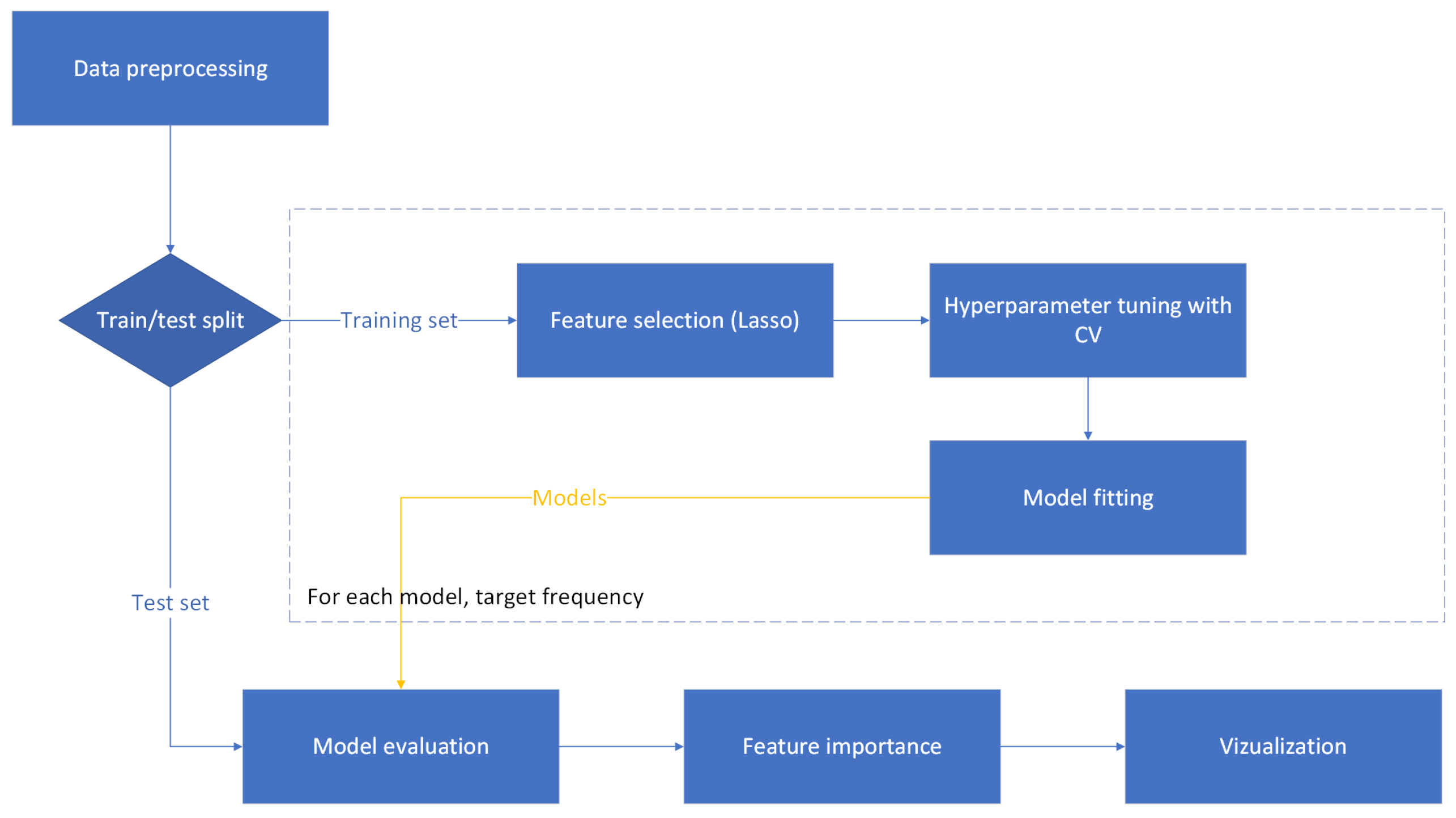
2.5. Experimental Setting 1: Hold-Out Method

In this setting, the model training and evaluation were performed with a separate training and test set. Feature importance assessment was performed on the testing set. The experimental scheme is illustrated in the Figure 2, with detailed steps outlined below. We describe only the processes specific to the hold-out method; general approaches are described in the previous sections.

1.

Data preprocessing

Value differences can be caused by different measurement techniques or units, which may magnify or obscure the importance of certain features. Data scaling was used to establish a consistent scale for the features. For categorical features, namely, gender and ear side, binary representation was used (e.g., male = 0 and female = 1). All other continuous values, both basic and constructed, were standardized to have a mean of 0 and a SD of 1. A portion of 20% of the data was randomly separated from the rest and used as a test dataset. Feature selection and training was performed on the remaining 80% of the data. The test dataset was used in the final evaluation.

2.

Feature selection

The reduction of redundancy introduced in feature engineering is achieved through the feature selection process, which aims to include only the most pertinent features for the given target. Limiting the number of features is also beneficial for decreasing computational time and improving interpretability [13].

In the Lasso regularization process, some coefficients are shrinked to zero. If there are highly correlated values, the Lasso tends to select one variable from each group and ignore the others [20]. This is essential, especially for feature importance estimation, since the permutation importance (PFI) [18] is estimated lower for strongly correlated features than for independent features [21,22]. Similarly, the presence of multicollinearity leads to unreliable estimation of Shapley values [23]. Shapley values are a core component of SHapley Additive exPlanations (SHAP) [24], another explainability method we used.

Additionally, Spearman correlation was computed on the Lasso-selected features to perform correlation analysis [25]. Collinear feature pairs were detected and the feature with the lower Lasso coefficient from the pair was removed from the selection.

3.

Hyperparameter tuning

The entire training set was used for hyperparameter tuning. The setting of tuning was cross-validated. The training set was split in 10 folds. Then, hyperparameters were selected based on CV performance.

4.

Feature importance

PFI was used to evaluate the importance of features. PFI does not suffer from the feature importance bias of the impurity importance, which can favor features with high cardinality [26]. To provide additional insight into the influence of each feature, SHAP analysis [24] was performed. Both explainability methods were applied to RF predictions on the test set.

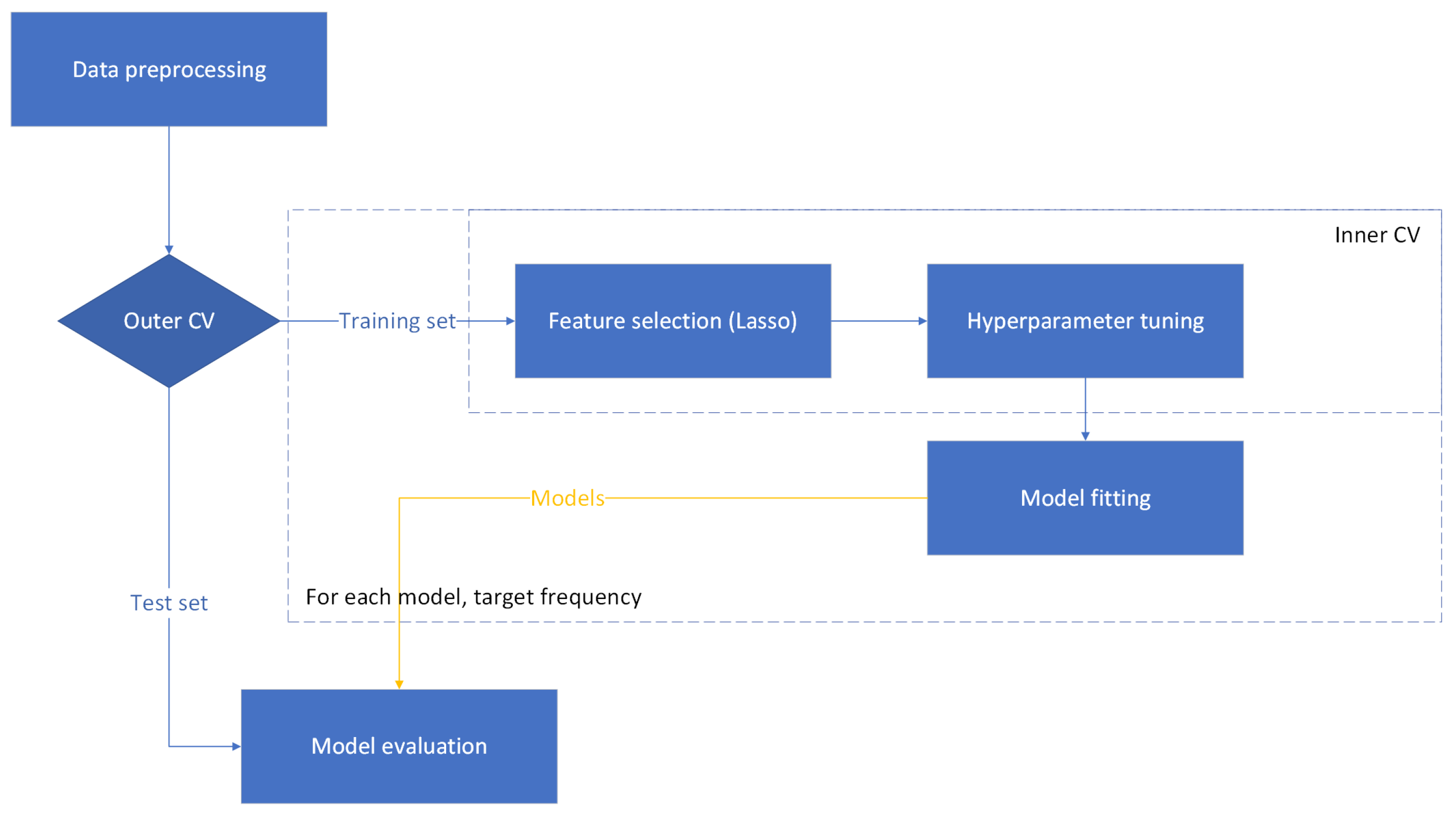
2.6. Experimental Setting 2: Nested CV

The evidence indicates that machine learning models based on the single hold-out method have low statistical power and confidence, which can result in overestimated classification accuracy [27]. Furthermore, the required sample size for the single hold-out method can be 50% higher than in cases of using nested k-fold CV [27]. Therefore, the nested CV setting can provide an experimental setting with increased statistical confidence. Nested CV was used in addition to the hold-out method to provide an alternative accuracy assessment.

The nested CV process is illustrated as a flow diagram in the Figure 3. Nested CV consisted of outer 4-fold CV and inner 3-fold CV. Standard selection for scaling and Lasso for feature selection were applied on the training data of given folds (in the process of inner or outer CV) to allow comparability to the hold-out method. The inner CV was responsible for feature selection and hyperparameter tuning. The best features and parameters were extracted from the inner CV, fit on the outer CV training data, and evaluated on the outer CV test fold. Naive methods were added as described in Section 2.4 and computed in the outer CV loop.

3. Results

3.1. Regression Evaluation: Hold-Out Method

In

Table 4. Prediction accuracy measures for each target hearing intensity. Results are presented as MAE ± SD. In the last column, the best result from naive methods is added for comparison. The best result per row is emphasized with bold font. Frequencies are in Hz. AC = air conduction; BC = bone conduction; KNNs = k-nearest neighbours; LR_all = linear regression with all features; RF = random forest; RF_all = random forest with all features.

Frequency	LR_all	Lasso	Ridge	KNNs	RF	RF_all	Naive
AC
125	10.65 ± 12.14	10.06 ± 11.94	10.08 ± 11.95	12.24 ± 13.69	10.47 ± 12.65	10.81 ± 12.98	12.21 ± 14.92
250	10.34 ± 13.45	10.81 ± 13.85	10.68 ± 13.67	10.56 ± 13.37	9.78 ± 12.59	10.07 ± 12.62	11.84 ± 15.50
500	8.23 ± 10.41	8.77 ± 11.24	8.72 ± 11.29	8.48 ± 11.41	8.42 ± 11.29	8.41 ± 11.64	10.73 ± 15.39
1000	5.60 ± 6.73	6.36 ± 7.61	6.43 ± 7.66	7.98 ± 9.64	7.02 ± 8.21	7.39 ± 8.69	11.12 ± 15.04
1500	5.19 ± 7.56	5.26 ± 6.89	5.00 ± 6.74	6.78 ± 9.05	5.05 ± 6.94	5.30 ± 7.15	10.23 ± 14.58
2000	6.13 ± 7.23	6.13 ± 7.55	5.86 ± 7.15	6.84 ± 7.94	5.07 ± 6.30	6.93 ± 8.02	11.53 ± 15.08
3000	6.94± 8.88	7.05 ± 8.70	7.19 ± 8.80	7.71 ± 10.03	7.43 ± 9.56	7.90 ± 9.88	14.52 ± 17.62
4000	10.21 ± 12.96	10.57 ± 13.03	10.41 ± 12.82	11.16 ± 14.33	9.15 ± 11.41	10.13 ± 12.96	14.8 ± 11.94
6000	12.47 ± 15.19	11.20 ± 13.97	11.47 ± 14.35	13.16 ± 16.70	11.24 ± 14.59	11.55 ± 14.94	10.60 ± 10.59
8000	15.03 ± 18.44	13.67 ± 16.63	13.92 ± 16.96	12.98 ± 16.16	13.62 ± 17.84	14.63 ± 18.50	11.80 ± 15.59
BC
500	3.89 ± 6.58	5.10 ± 8.26	5.00 ± 8.36	5.04 ± 9.53	4.75 ± 8.74	4.90 ± 8.66	5.60 ± 9.29
1000	3.85 ± 5.45	4.73 ± 6.73	4.67 ± 6.71	4.8 ± 7.01	4.67 ± 7.09	4.68 ± 8.66	6.0 ± 8.60
1500	5.04 ± 6.11	5.66 ± 6.99	5.41 ± 6.67	5.80 ± 7.49	5.34 ± 6.79	4.59 ± 6.10	5.40 ± 7.36
2000	5.48± 6.67	5.74 ± 7.21	5.60 ± 6.95	7.0 ± 8.48	5.53 ± 6.63	6.20 ± 7.34	6.20 ± 8.28
3000	5.63 ± 7.21	5.48 ± 7.26	5.44 ± 7.21	6.48 ± 8.14	5.55 ± 7.56	6.13 ± 7.58	6.20 ± 7.91
4000	5.26 ± 6.42	4.90 ± 6.37	4.90 ± 6.37	5.74 ± 6.36	4.35 ± 5.62	5.43 ± 6.86	4.20 ± 6.08

, the accuracy scores (MAE ± SD) of the five different models trained with the hold-out method are presented along with the RF without feature selection and best naive predictions column.

Considering only the naive predictions, in the first seven rows (including the 3000 Hz frequency), the naive approach y_average, which includes the average of all postoperative samples at the chosen hearing intensity, performed best. In all other rows, the naive method x, which takes the preoperative hearing level at the same frequency as its prediction, performed best. Their MAE values are given in the rightmost column of Table 4.

LR_all achieved the lowest MAE scores in a total of six cases. For AC frequencies 500, 1000, and 3000 Hz, MAEs of 8.23, 5.60, and 6.94 were recorded. For BC frequencies 500, 1000, and 2000 Hz, MAEs of 3.89, 3.85, and 5.48 were achieved. RF was the best performing model for predicting the postoperative AC hearing intensity for three targets: at 250 Hz with MAE of 9.78, at 2000 Hz with MAE 5.07 and at 4000 Hz with MAE 9.15. Ridge was the best performing model for predicting the postoperative hearing intensity in two cases: at 1500 Hz AC with an MAE of 5.00 and at 3000 Hz BC with MAE 5.44. Lasso attained the lowest MAE of 10.06 for AC hearing at 125 Hz. RF_all was most accurate in one BC frequency with 4.59 MAE at 1500 Hz. Naive prediction approaches also performed best for three high frequency targets. MAEs of 10.60 and 11.80 were observed for AC frequencies 6000 and 8000 Hz. An MAE of 4.20 was achieved for the BC frequency at 4000 Hz. For the KNNs model, consistently higher MAE values were measured. Consequently, it was not the best performing model for any of the targets.

SD values were higher than MAE in all cases. There was no significant difference in SD between the models. The model with the best MAE normally also achieved the lowest SD. However, exceptions occurred for AC and BC frequencies at 3000 and 2000 Hz, where lower SD values were observed for Lasso (7.05 ± 8.70) and RF (5.53 ± 6.63) than for the model with the lowest MAE—LR_all (6.94 ± 8.88, 5.48 ± 6.67), respectively.

Figure 4 visualizes the audiogram measurements on a test sample together with the postoperative predictions. The predictions for each target are illustrated as AC and BC vectors. The poor prediction accuracy at high AC frequencies is evident from the graph, an observation consistent with the overall accuracy at these frequencies.

3.2. Regression Evaluation: Nested CV

In

Table 5. Prediction accuracy for each target hearing intensity for CV (outer split). Results are presented as MAE ± SD. In the last column, the best result from naive methods is added for comparison. The best result per row is emphasized with bold font. Frequencies are in Hz. AC = air conduction; BC = bone conduction; KNNs = k-nearest neighbours; LR_all = linear regression with all features; RF = random forest; RF_all = random forest with all features.

Frequency	LR_all	Lasso	Ridge	KNNs	RF	RF_all	Naive
AC
125	10.25 ± 12.55	8.90 ± 10.95	8.86 ± 10.92	9.54 ± 11.58	9.48 ± 11.40	9.48 ± 11.20	10.51 ± 12.65
250	8.81 ± 11.05	8.08 ± 10.30	8.36 ± 10.48	8.32 ± 10.55	8.42 ± 10.69	8.22 ± 10.43	9.16 ± 12.01
500	7.88 ± 10.20	7.34 ± 9.61	7.40 ± 9.65	7.71 ± 9.89	7.53 ± 9.81	7.37 ± 9.64	9.02 ± 11.73
1000	6.94 ± 8.46	7.04 ± 8.11	6.95 ± 8.00	7.33 ± 8.99	6.90± 8.11	7.04 ± 8.50	9.11 ± 11.61
1500	6.53 ± 8.81	5.77 ± 7.97	5.69 ± 7.81	6.75 ± 8.96	5.93 ± 8.19	5.97 ± 8.21	9.75 ± 12.90
2000	6.44 ± 7.95	5.86 ± 7.40	5.89 ± 7.41	6.15 ± 7.84	5.61 ± 7.36	6.26 ± 7.93	11.36 ± 14.12
3000	7.52 ± 9.54	6.92 ± 8.52	6.97 ± 8.57	8.83 ± 10.17	7.42 ± 9.16	7.49 ± 8.98	14.31 ± 16.51
4000	8.64 ± 11.73	8.55 ± 11.12	8.41± 11.17	9.44 ± 11.86	9.10 ± 11.64	8.81 ± 11.33	15.70 ± 18.58
6000	10.90± 14.94	11.26 ± 14.15	11.00 ± 14.16	12.90 ± 15.45	11.34 ± 14.29	11.39 ± 13.97	14.90 ± 15.40
8000	14.08 ± 18.16	12.46 ± 16.03	12.47 ± 16.26	13.32 ± 17.10	13.16 ± 17.06	13.95 ± 17.76	12.26± 16.36
BC
500	3.61 ± 4.85	3.62 ± 5.17	3.72 ± 5.02	3.22 ± 5.53	3.23± 5.17	3.51 ± 4.96	4.79 ± 6.67
1000	4.44 ± 5.91	3.87 ± 5.22	3.98 ± 5.26	4.43 ± 6.07	4.36 ± 6.17	4.58 ± 6.11	5.20 ± 6.16
1500	5.53 ± 7.39	5.41 ± 7.02	5.54 ± 7.18	6.72 ± 8.60	5.85 ± 7.64	6.07 ± 7.84	6.79 ± 8.03
2000	6.25 ± 8.19	5.62 ± 7.38	5.65 ± 7.52	6.28 ± 8.06	6.36 ± 8.24	6.25 ± 8.09	6.39 ± 8.45
3000	6.05 ± 7.64	5.30 ± 6.85	5.30 ± 6.80	6.51 ± 7.92	6.02 ± 7.62	6.20 ± 7.55	5.70 ± 7.36
4000	6.13 ± 8.36	5.72 ± 7.70	5.72 ± 7.77	6.74 ± 8.55	6.04 ± 7.92	6.53 ± 8.43	5.21 ± 7.66

, the accuracy scores (MAE ± SD) of the five different models trained by nested CV are presented along with the RF without feature selection and best naive predictions column.

For the naive predictions in nested CV, in the first eight rows (including the 4000 Hz frequency), the naive approach y_average performed best. In all other rows, the naive method x was best performing. Their MAE values are given in the rightmost column of Table 5.

Lasso attained the highest MAE scores in a total of seven frequencies. For AC frequencies 250 Hz, 500 Hz, and 3000 Hz, MAEs of 8.08, 7.34, and 6.92 were recorded. In predicting BC frequencies, Lasso was most successful at frequencies 1000 Hz, 1500 Hz, 2000 Hz, and 3000 Hz with MAE scores of 3.87, 5.41, 5.62, and 5.30. Ridge had the highest prediction accuracy for AC hearing at 125 Hz, 1500 Hz, and 4000 Hz with MAEs 8.86, 5.69, and 8.41. RF demonstrated the lowest MAE scores among all considered models at AC frequencies 1000 and 2000 HZ and a BC frequency of 500 Hz. MAE values of 6.90, 5.61, and 3.23 were achieved at these frequencies. LR_all model achieved the lowest MAE value (10.90) at an AC frequency of 6000 Hz. Naive prediction approaches performed best for two of the highest AC and BC frequency targets. Specifically, an MAE of 12.26 was observed for AC frequency 8000 Hz, and an MAE of 5.21 was observed for BC hearing at 4000 Hz.

Higher dB values were observed for SD than MAE in all occurrences. No significant differences between SDs were observed, with the most accurate models in terms of MAE typically achieving lower standard deviation values. However, some target frequencies can be found where SD was lower for models that did not achieve the highest MAE. For example, Ridge (6.95 ± 8.00) had lower SD than RF (6.90 ± 8.11) for AC hearing at 1000 Hz. Lasso (8.55 ± 11.12, 11.26 ± 14.15) achieved lower SD values than Ridge (8.41 ± 11.17) and LR_all (10.90 ± 14.94) for high frequency AC hearing at 4000 and 6000 Hz. Similarly, Lasso (12.46 ± 16.03) had lower SD than the naive method x (12.26 ± 16.36) for predicting AC hearing intensity at 8000 Hz. For bone conduction, a lower SD was observed for LR_all (3.61 ± 4.85) than for RF (3.23 ± 5.17) at frequency 500 Hz.

Comparing results of the two training methods used, namely, the hold-out method (Table 4) and nested CV (Table 5), several differences were observed. Overall better accuracy scores were achieved with nested CV at AC frequencies 125 Hz, 250 Hz, 500 Hz, 3000 Hz, and 4000 Hz, as well as at BC frequencies of 500 and 3000 Hz. Worse scores were observed at other frequencies. The model performance also differed significantly. While the LR_all model was the best performing in the hold-out context, with best scores at six frequencies, it was ranked among the worst models during nested CV training. The model that demonstrated the best performance in the nested CV setting was Lasso.

3.3. Feature Importance

In this section, the feature importance results are discussed. If the type of hearing intensity is not specified in the text (preoperative/postoperative), it can be assumed to be preoperative. Only preoperative hearing intensities are part of feature sets and are therefore referenced frequently.

To extract the features that are informative overall,

Table 6. Top 5 most frequently selected features. ABG = air–bone gap; xBefAir = preoperative air conduction hearing intensity at frequency x; xBefBone = preoperative bone conduction hearing intensity at frequency x.

Feature	Number of Occurences
8000BefAir	10
500BefAir	7
ABG	7
4000BefBone	5
1000BefBone	5

contains the top five most frequently selected features from the feature selection process on all targets. The high frequency AC value at 8000 Hz was chosen in the feature selection process in 10 out of 16 cases. AC hearing measurements at 500 Hz and ABG were selected for the prediction of seven targets. BC hearing intensities at 1000 and 4000 Hz were both selected five times.

The following graphs show a comparison of feature importance analyses on four different targets. One high-frequency and middle-frequency target hearing intensity was compared for AC and BC, primarily to investigate the poorer prediction accuracy of high frequencies at the feature level. Feature importance graphs for predicting hearing at other frequencies are available in the Supplementary Files (PFI plots in S1 and SHAP plots in S2).

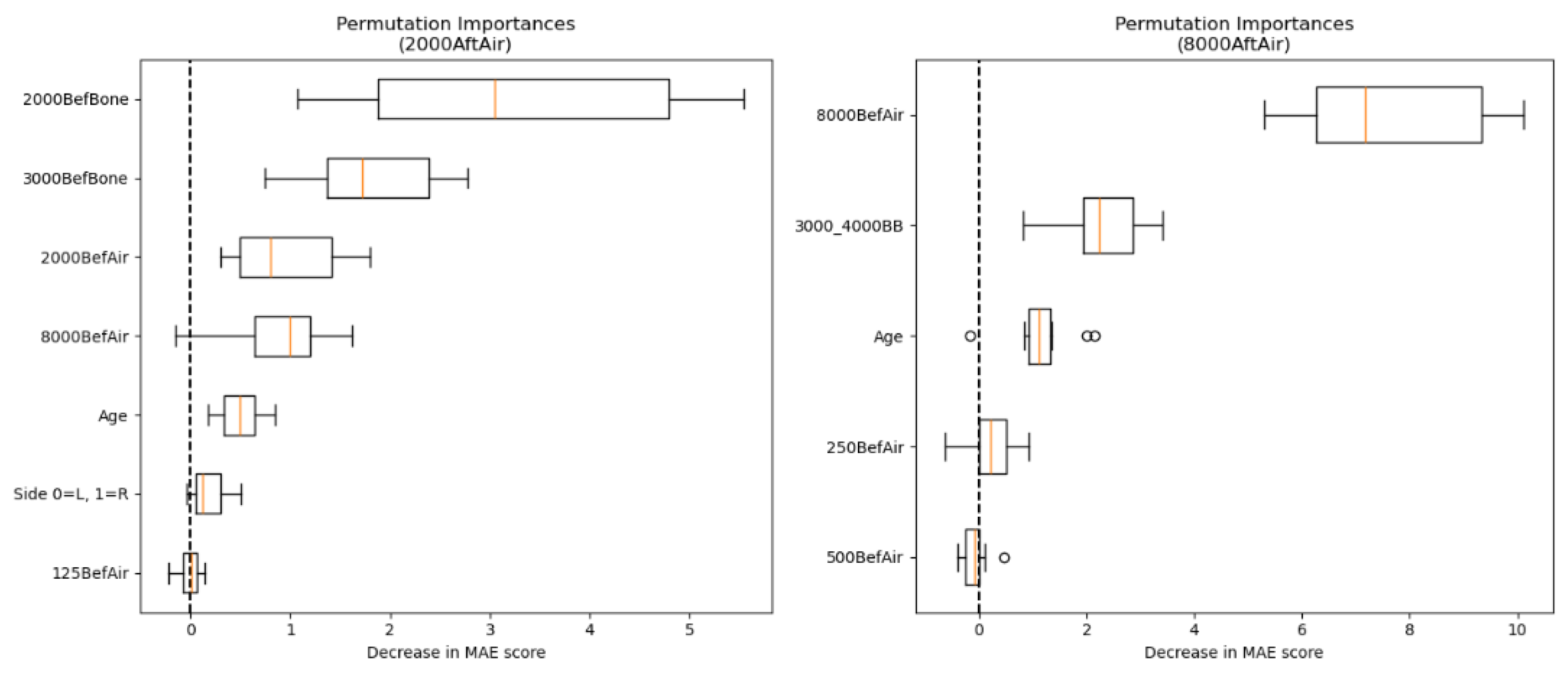
PFI box plots show a decrease in MAE when randomly permuting each individual feature. If the model performs the same or better when a feature is randomly permuted, this indicates that the feature does not provide significant value to the prediction. Figure 5 contains a side-by-side comparison of the PFI for predicting AC hearing intensity at frequencies 2000 and 8000 Hz. The most significant features in the prediction of AC targets at 2000 Hz were the BC values at frequencies 2000 and 3000 Hz. A considerable impact was also observed for AC hearing intensities at frequencies 2000 and 8000 Hz, and age. Ear side and 125 Hz AC value had a negligible effect on prediction.

When predicting the postoperative AC hearing intensity at 8000 Hz, the preoperative AC hearing intensity at 8000 Hz had the largest effect on successful prediction. Other relevant features were the combined BC hearing intensity at frequencies 3000 and 4000 Hz and age. AC value at the frequency 250 Hz was of limited predictive value, whereas random permutation of AC at 500 Hz mostly did not reduce the MAE.

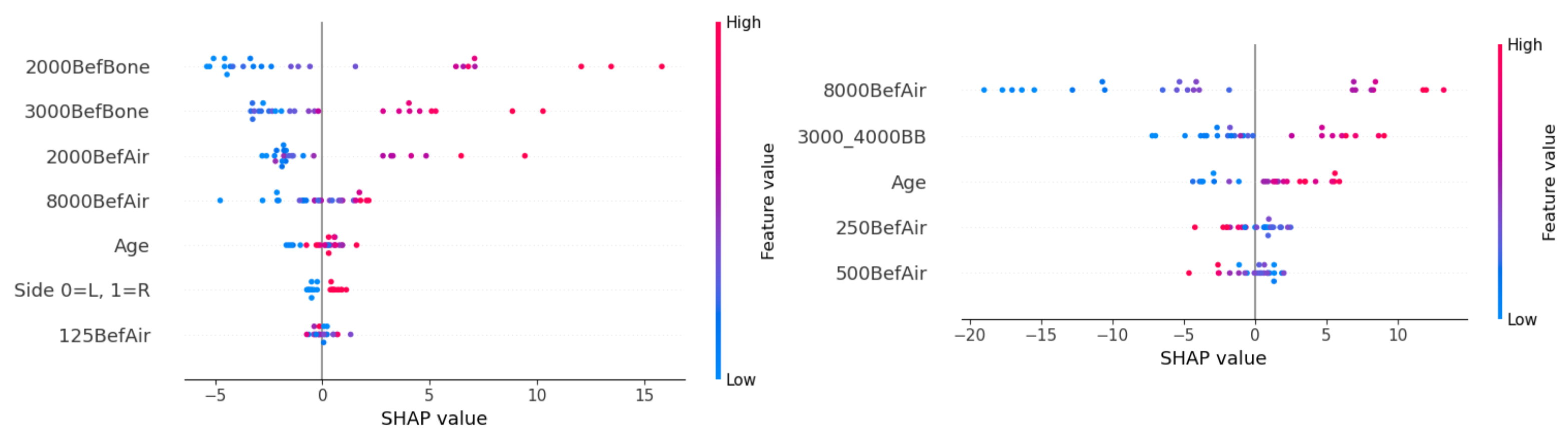
The SHAP feature directionality is shown in Figure 6. For the prediction of postoperative AC hearing at 2000 Hz, worse preoperative hearing at BC frequencies 2000 and 3000 Hz, as well as at AC frequencies 2000 and 8000 Hz, contributed to worse hearing prediction (higher dB values). Surgery on the right ear and young age were associated with better postoperative hearing. For the feature AC hearing at 250 Hz, the directionality cannot be clearly determined from the graph.

Young age also had a better prognosis for the prediction of postoperative AC hearing at 8000 Hz. Higher feature values for AC hearing at 8000 Hz and combined BC hearing at 3000 and 4000 Hz had high SHAP values, causing worse postoperative hearing. Low values of AC hearing intensity at 8000 Hz show a significant impact on postoperative hearing. If low dB hearing intensities were observed preoperatively, they are likely to remain low postoperatively. Interestingly, for AC hearing at 250 and 500 Hz, the opposite influence can be observed—the model predicted lower (better) postoperative hearing intensity for individuals with worse preoperative hearing. However, the validity of this finding is questionable, as these two features have a limited impact on successful prediction (see Figure 5).

Figure 7 presents a side-by-side comparison of the PFI for predicting BC hearing intensity at frequencies of 1500 and 4000 Hz. The most significant feature in predicting the postoperative BC hearing intensity at 1500 Hz was the preoperative BC value at the same frequency. Other useful features were the combined BC hearing intensities at 3000 and 4000 Hz, as well as the BC hearing at 1000 Hz and AC hearing at 8000 Hz. The gender and ABG of patients had a negative impact on successful prediction based on PFI.

For predicting target BC at 4000 Hz, the preoperative hearing at the same frequency had the most significant effect. AC hearing at 8000 and 4000 Hz also had a considerable impact. A small reduction in MAE was observed when ABG and AC hearing at 500 Hz were randomly permutated.

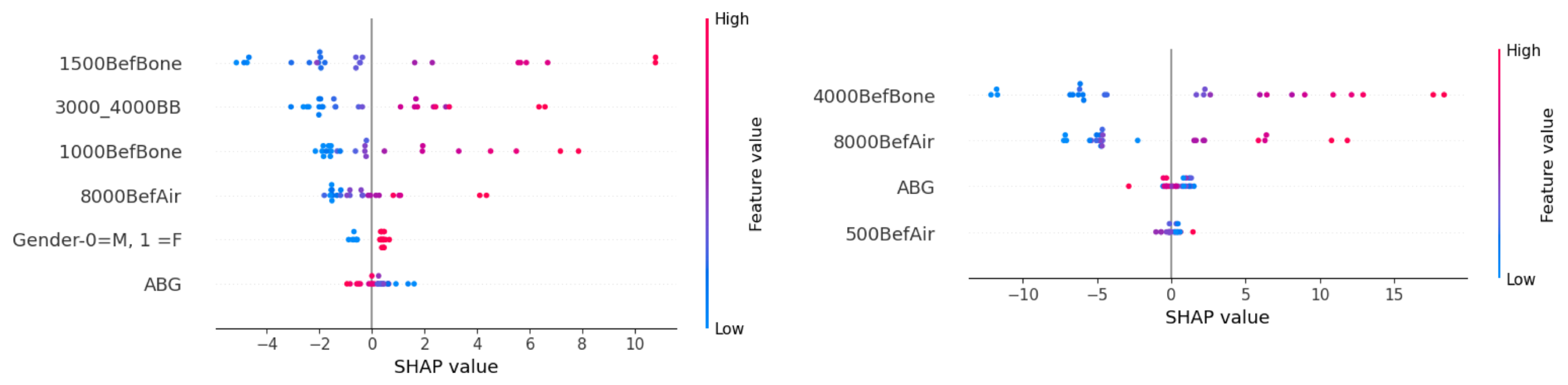
SHAP values for individual features are presented in Figure 8 below. High preoperative hearing intensities, namely at BC frequencies of 1500 and 1000 and at combined frequencies of 3000–4000 Hz, together with the AC at 8000 Hz, showcase higher values for the prediction target. The model associated female individuals and low ABG with higher postoperative hearing intensity. Since the importance of these values is low according to Figure 7, the mentioned feature directionality for gender and ABG did not contribute to more accurate predictions.

A similar pattern was observed when predicting the BC hearing at 4000 Hz. Worse BC hearing at the frequency 4000 Hz and AC hearing at the frequency 8000 Hz resulted in higher hearing intensity predictions. Lower ABG was associated with poorer postoperative hearing predictions. The directionality of AC hearing at 500 Hz is ambiguous.

4. Discussion

While it is difficult to assess the obtained results due to the shortage of hearing recovery prediction methods after stapedotomy, it is possible to compare the findings with hearing recovery prediction approaches of other surgeries or illnesses. Most of the existing approaches are classification-based—the models are trained to predict whether hearing recovery will be achieved or not. The existing approaches evaluate hearing recovery either by Siegel’s criteria [4,5,6,7] or thresholding based on PTA or ABG [8,9]. In our case, we aimed to accurately predict each postoperative hearing intensity. The hearing recovery level can be extracted from the audiogram estimate. It is hypothesized that estimating an entire postoperative audiogram provides more informativeness for stapedotomy prognosis.

Since the single hold-out method has been shown to have low statistical power and high bias [27], regression results from training the models in nested cross-validation will be given higher importance when discussing regression results. The single hold-out method has provided value as an independent benchmark for model evaluation and further in the process for feature importance estimation.

Considering the nested CV setup, the regression results indicate that the hearing intensities at border frequencies (8000 Hz AC, 4000 Hz BC) are notably more difficult to predict, given the superior performance of the naive model, which predicts no change from preoperative hearing. Furthermore, the models demonstrated mediocre quality for predicting values at high frequencies of 6000 Hz AC and 3000 Hz BC with MAE values below, but in close proximity to, the naive predictions. Initial hearing intensities at given frequencies have the highest variance, which could result in challenging prediction. Prediction of low-frequency AC hearing levels (125 Hz, 250 Hz, 500 Hz) also proved to be difficult with models achieving MAE values of around 8 dB. A lower MAE was observed for BC hearing targets, as the targets rarely deviated significantly from the preoperative values. The best prediction accuracy was achieved for the most crucial AC hearing frequencies 1000, 1500, 2000, and 3000 Hz.

Among the models trained during the nested CV, Lasso performed best overall, considering the limitations of all models discussed in the previous paragraph. It should be noted that naive methods achieved best results at border frequencies (8000 Hz AC, 4000 Hz BC), indicating a poor prediction quality of all machine learning methods at these frequencies. The efficiency of feature selection and regularization approaches was demonstrated in the results, as Lasso and Ridge outperformed LR_all with all features for 13 out of 16 targets. Ridge and RF methods provided prediction accuracy comparable to Lasso. The success of linear models can be attributed to the linear relationship between preoperative and postoperative data. The superiority of Lasso and Ridge can also be due to the previous usage of Lasso in the feature selection. However, RF with all features did not achieve better results than other methods for any frequency, which further implies the feature selection benefits. KNNs was consistently the worst prediction model. This may indicate that the audiogram data are not well separated and, therefore, prediction based on feature proximity is not suitable.

Feature importance based on the selection frequency for the prediction of different targets indicates an overall significance of high-frequency AC hearing at 8000 Hz. Based on the four closely analyzed targets, AC hearing at 8000 Hz consistently delivers value in the prediction of both AC and BC targets. The number of feature occurrences can be misleading for feature importance evaluation. For example, AC hearing intensity at 500 Hz was selected seven times. However, randomly permuting it in two analyzed cases only led to minimal MAE score decrease. Further insight into feature importance was provided by PFI and SHAP analyses. In all four analyzed examples, the preoperative hearing at the same frequency as the target was the most important feature. Nevertheless, the main difference in predicting the AC hearing at 2000 and 8000 Hz was the conduction type of the most significant hearing intensity feature. At 2000 Hz, the preoperative BC was most impactful, whereas at 8000 Hz, the preoperative AC was the most valuable. This finding indicates that preoperative BC values are significant mainly for the prediction of AC between 500 Hz and 4000 Hz, serving as a limit in the ABG reduction. The SHAP analysis revealed that the lower preoperative hearing intensity values resulted in lower hearing intensity predictions. Young age was generally associated with better postoperative hearing.

Feature importance can be compared to other hearing recovery prediction approaches. It should be noted that the significance of features for hearing recovery may vary depending on the surgical procedure or underlying medical condition. The importance of hearing intensity features has been widely reported; however, some authors aggregate these features (for example, as PTA). The significance of preoperative high frequency hearing at 8000 Hz was recognized also in the case of ISSHL hearing recovery [5,6,7]. Furthermore, the importance of BC frequencies was observed in mastoidectomy hearing recovery prediction [9]. While age and ABG had a considerable influence on the prediction in our case, they were not among the most important factors, as they were in some previous studies [8,9]. In our case, the ABG influence may have been diminished by the effect of other hearing intensity features. In our approach, the analysis of the influence of features for single hearing intensity prediction was enabled, in contrast to previous work.

Our method is applicable as a decision support for stapedotomy surgery or potentially in any setting where audiogram estimation is required. In its current state, this system can be adapted and trained on isolated surgical data from a single surgeon. The drawback of focusing on a single surgeon is that the operating surgeon must perform a large number of operations with consistent results and comparable surgery settings to collect enough data. Only then is the model able to learn valuable insights, since inconsistent surgery performance or settings could lead to data of inadequate quality. Future studies could incorporate multi-surgeon and multi-center data to enhance the external validity and improve generalizability. Nevertheless, to create a more general machine learning system, other factors such as device type, surgical technique, etc., would need to be considered. Limitations of this study include the small number of patients and features. Although preoperative hearing intensities are consistently among the most significant features for hearing recovery prediction [4,5,6,7,8,9], other factors influence the outcome in stapedotomy—primarily, the anatomical conditions in the middle ear (location of the long process of the incus ossicle, a dehiscent facial nerve, which narrows the oval window niche and thickness of the stapedial footplate).