Enhanced Blind Separation of Rail Defect Signals with Time–Frequency Separation Neural Network and Smoothed Pseudo Wigner–Ville Distribution

Abstract

Railways are crucial in economic development and improving people’s livelihoods. Therefore, defect detection and maintenance of rails are particularly important. In order to accurately separate and identify the rail defect from the mixed signals by acoustic emission (AE) techniques, this paper proposes a novel time–frequency separation neural network (TFSNN) architecture to solve the problems existing in the blind source separation (BSS), such as in non-stationary signals and low stability in the convergence. Combined with the smoothed pseudo Wigner–Ville distribution (SPWVD), this method can increase the spectrogram resolution, suppress the noise interference, and effectively improve the extraction performance of crack signals. In addition, 1D-CNN and GRU structures were introduced in the TFSNN structure to exploit the dominant features from AE signals. A dense regressor was also subsequently used to estimate the separation weights. Simulation and experiments showed that compared with traditional algorithms like independent component analysis, shallow neural networks, and time–frequency blind source separation, the proposed algorithm can provide better separation performance and higher stability in rail crack detection.

1. Introduction

Over the past decades, high-speed rail has undergone rapid development, and it has become a popular mode of transportation for intercity and cross-regional travel. With its speed, safety, and convenience, high-speed railways have significantly reduced the travel time between cities and fostered economic and cultural exchanges. A number of countries have constructed high-speed rail infrastructures to improve their technical level and service quality. However, during daily train operations, various damage, such as cracks, spalling, shelling, and fractures, often occur on the rails, severely affecting operational safety [1]. Therefore, it is necessary to strengthen the overhaul and maintenance of steel rails to ensure the safe operation of high-speed railways.

At present, traditional defect detection methods for critical structures in high-speed railways struggle to identify internal or early-stage defects due to blind spots, low sensitivity, and other issues. Therefore, acoustic emission (AE) technology has drawn increasing attention; it collects and analyzes acoustic signals passively to achieve fast and accurate detection of rail cracks, with its natural advantages of high sensitivity and real-time detectability [2]. However, there normally exist complex noise components in the actual railway environment. The acquired AE signals need to be denoised or demixed before the defect source can be identified, and blind signal separation (BSS) technology is thus introduced in this study to effectively extract the crack signal from the received acoustic mixtures.

Blind signal separation (BSS) is a powerful multi-channel signal processing technique that offers non-parametric optimization and requires no prior knowledge of the mixing process or source signals. Considering their strong capability and flexibility in separating the acoustic mixtures, BSS algorithms have been studied in depth by the research community and broadly applied in industrial or medical fields, such as in fault diagnosis in bearings/gearboxes [3], EEG/ECG event extraction [4], wireless communication [5], and speech separation, enhancement, and dereverberation [6]. Independent component analysis (ICA) is one of the most cited BSS methods that originated from multi-sensor processing, and it retrieves the demixing weights through maximizing the independence or the non-Gaussianity of the demixed signals. For example, Maddirala presented a singular spectrum analysis integrated with ICA technique for single-channel EEG signal separation [7]. However, the traditional ICA method has a low separating accuracy in the existence of non-stationary noise or high amplitude Gaussian noise. To solve this problem, Mohanaprasad et al. modified the adaptive ICA into a noise cancellation method for a speech signal in communication devices. The simulation results showed that the interference of the noise is significantly reduced in the proposed method [8]. Aside from ICA, there is also another representative branch of BSS methods based on the statistic metrics, i.e., joint approximate diagonalization of eigenmatrices (JADE) and second order blind identification (SOBI). Jian proposed an improved SOBI method involving a Hilbert transform for blind identification of bandlimited signals [9]. Theoretically, JADE makes use of the fourth order cumulants to automatically suppress Gaussian background noises and enhance non-Gaussian sources. To cope with the problem when two subjects of Doppler radar cross the angular resolution limit, Chowdhury et al. introduced JADE into the array signal processing of radar, and experimental results demonstrated JADE superseded the performance of the other extraction methods [10].

However, conventional BSS methods rely highly on the optimization process with a recursive fixed-step quasi-Newton method, which is inefficient and suffers from slow computing, oscillation, and instability of the convergence. In consequence, this situation might cause an inaccurate or low steady-state separation performance for the targeted source even if the computing or tracking process is sufficiently long [11]. Instead, the implementation of neural networks or artificial intelligence algorithms in BSS could avoid this deficiency and have the advantage that the objective function and optimization algorithm are independently assigned. In this way, the optimization algorithm can be flexibly combined with different criteria such as batch processing and variable step-size learning, according to the actual demand [12]. In addition, finding network computing and computational intelligence implementations of BSS is of great necessity for it could increase the robustness of the separation algorithms in contrast with a linear separation method such as ICA, eliminating the uncertainties and ambiguities in the real-world sources.

For instance, Isomura et al. advanced a shallow neural network-based separation method, which is updated by the error-gated Hebbian rule and suitable for multi-context blind source separation simultaneously [13]. Liu designed a biased dense neural network on the basis of a maximum likelihood estimation criterion in order to obtain a better steady-state separating performance [14]. Particularly, in light of temporal convolutional encoder and weighting masks, a convolutional time-domain audio separation network (Conv-TasNet) was proposed by Luo and Mesgarani for single-channel or underdetermined speech separation tasks [15]. Conv-TasNet sufficiently exploited the time–frequency spectrogram for speech signals and output the probabilistic masking, but it cannot perfectly reconstruct the source signals when they have obvious frequency overlapping. Sinha proposed a LSTM variant single target speaker extraction method, composed of a speaker embedder and separator networks [16]. Lee employed an end-to-end W-shaped network to extract a fetal ECG signal, but it is a dual-path structure and can only be utilized in two channels [17]. Although the neural network-based BSS methods endorse the overall separating performance under different application scenarios, when applied in actual railway environments, the BSS technology still confronts the specific non-stationary and time-varied spectral characteristics of complicated noisy signals. Due to this, accurately extracting the target signal in the actual railway, such as with a rail defect signal, remains an intractable challenge. In this case, the time–frequency analysis (TFA) plays a pivotal role in characterizing the non-stationary signal attributes across time and frequency domains [18]. There are two primary approaches to incorporate TFA into blind source separations. Firstly, in an undetermined BSS scenario, discrete TFA techniques can be employed to decompose the insufficient observations into a set of resolved signals. For instance, Massar compared variational mode decomposition (VMD) and discrete wavelet transform (DWT) in decomposing the single-channel signal when combined with ICA and found that VMD demonstrated slightly higher effectiveness [19].

Secondly, given that BSS techniques can be utilized in both image and signal separation, continuous TFA or spectrograms can serve as direct inputs for estimating the separation weights. Such TFA approaches provide a comprehensive understanding of signal dynamics that surpasses conventional BSS techniques focusing solely on temporal or spectral domains. Cheng et al. combined a short-time Fourier transform (STFT) with convolutive BSS to calculate more reliable unmixing filters [20]. But, according to Heisenberg’s uncertainty principle, the STFT suffers from the limited TF resolution and information loss caused by linear TF conversion and the fixed window functions. In this regard, a continuous wavelet transform (CWT) can be used in BSS to give a higher resolution representation with scalable windows. However, a CWT is significantly influenced by the choice of the mother wavelet, which requires considerable effort to select in practice [21]. As an alternative, a Wigner–Ville distribution (WVD) and Cohen’s class can also be used in TFA feature extractions for BSS, with a sparser spectrogram, better energy concentration, and separation performance on the basis of quadratic TF conversion [22]. Particularly, Cohen’s class methods, such as the Choi–Williams distribution (CWD), were reported to be able to effectively remove cross interferences in a noisy environment and make a more robust representation result [23].

Therefore, this paper proposes a defect signal extraction method based on time–frequency blind source separation algorithms and enhanced adaptive neural networks. By Wigner–Ville mapping the one-dimensional signal in the time domain to the two-dimensional time–frequency domain, the information of the temporal spectrum is reflected, and then the time–frequency features are separated with a specific designed adaptive neural network so as to realize the effective separation of the crack signal and noise signals. Section 2 presents the theoretical basis and details of the proposed methodology of a time–frequency separation neural network. Section 3 introduces the acquisition of the dataset and the experimental test. In Section 4, the defect detection performance of the proposed method with the simulated test signal and the experimental test signal were validated to supersede the compared methods, and then comparison of methods in the whole test set was systematically evaluated. Section 5 gives the concluding remarks.

2. Methodology of Time–Frequency Separation Neural Network

2.1. Basic Blind Source Separation Problem and Typical Solutions

Blind source separation (BSS) originated from the “cocktail party problem”, which is initially a term related to speech recognition, aiming to separate a target individual signal from multi-channel speech mixtures. Theoretically, the aim of BSS is to seek out the estimated source signals using only the observed signals from the recording devices, without any prior information of the source signals or mixing parameters of the channels. Blind source separation problems can be categorized into four types based on the hypothetical mixing models involved, as shown in Figure 1. This article mainly focuses on the instantaneous linear mixing model, which is illustrated as follows:

Supposing there are n unknown source signals, which are statistically independent of each other, after passing through a certain linear system, they are mixed and then captured by m devices, resulting in m mixed signals in the linear instantaneous mixing model. The relationship between the mixed signals and the source signals can be expressed as

$$x(t)=As(t)+n(t)$$

(1)

The matrix, $A={[a_{ij}]}_{m\times n}(i=1,2,\dots ,m;j=1,2,\dots ,n)$, is called the mixing matrix, $a_{ij}$ representing the unknown mixing coefficients, and $n(t)$ is the additive white noise in the mixing process. Then, BSS is used to obtain estimates of the source signals from the mixed signals $y(t)={[y_1(t),y_2(t),\dots ,y_n(t)]}^T=\widehat{s}(t)$. If matrix A is invertible, namely that the number of observations is equivalent to or larger than the number of sources, this objective can be completed with a separation matrix $W=A^{-1}$.

$$y(t)=Wx(t)=WAs(t)=\widehat{s}(t)$$

(2)

Therefore, the BSS problem can be summarized as seeking a separation matrix W or projection vectors to linearly combine the mixed noisy signals and obtain estimated signals that are as mutually independent as possible, as shown in Figure 1. One of the major assumptions related to BSS is the statistical independence of the primary sources, which leads to the solution of the independent component analysis (ICA) method. According to the central limit theorem, under the hypothesis of independent and identically distributed variables, the characteristics of mixed signals are closer to a Gaussian distribution than those of individual source signals. Then non-Gaussianity metrics such as negentropy and kurtosis can be utilized as measures of statistical independence in BSS. When negentropy is used, as shown in Equation (3), the separation vector $W^{*}$ with a maximal metric indicates the highest probability of independent sources.

$$\left\{\begin{array}{l}{W}^{*}=\underset{W}{\arg \max }{\left\{H\left(y_{Gauss}\right)-H\left(y\left(t\right)\right)\right\}}^2\approx \underset{W}{\arg \max }C{\left\{E\left[G\left(y_{Gauss}\right)\right]-E\left[G\left(y\left(t\right)\right)\right]\right\}}^2\\ H\left(y\right)=-{\displaystyle \int p\left(y\right)\log p\left(y\right)dy}\end{array}\right.$$

(3)

where $y_{Gauss}$ is a random vector composed of n Gauss variables, which has the same mean values and covariance matrices as variable $y\left(t\right)=Wx\left(t\right)$. $H\left(\cdot \right)$ is the negentropy, rigorously defined as Equation (3). In addition, the derivative of $H\left(\cdot \right)$ is the cumulative distribution function (CDF) of observed variables, which should be monotonically increasing in the range of [0, 1]. Accordingly, there are also three typical approximate estimate functions for $H$, $G_1\left(y\right)=y^3/4$, $G_2\left(y\right)=1-\exp \left(-y^2/2\right)$, $G_3\left(y\right)=1/a\log \cosh \left(ay\right)$, $1\le a\le 2$. The ICA method has been universally acknowledged as an efficient BSS method, and it is thus used as the first compared method in this paper, and the third approximate estimate function is selected according to the suggestion in a previous work [24]. However, in a standard ICA process like FastICA, the objective of negentropy is recursively optimized with a fixed-step quasi-Newton method, which might suffer from slow computing, oscillation, and instability of the convergence [11]. Therefore, a modified version of ICA is proposed in this paper in the next section to overcome the aforementioned disadvantages. Furthermore, the BSS problem is not limited to speech, and the processing or recovery of the other types of data might also include BSS techniques, such as complex signals and images. This characteristic makes it possible to introduce time–frequency analysis for the original acoustic signals before applying the BSS algorithm.

2.2. Time–Frequency Analysis of AE Signals Using Smoothed Pseudo Wigner–Ville Distribution

Due to the non-stationary and time-varying spectral characteristics of crack and abnormal noise signals, classical blind source separation algorithms may not be able to accurately extract the source signal, resulting in aliasing and noticeable degradation in separation performance. For non-stationary signals, the time–frequency analysis (TFA) plays a pivotal role in characterizing signal attributes across time and frequency domains [18]. Using TFA, time–frequency conversion between the mixed signals should be achieved before various separation schemes of the mixed chaotic AE signals.

Therefore, the first key step of the proposed algorithm is to perform time–frequency conversion on the mixed signal, and the final separation performance will naturally be different depending on the adopted TFA method. Wigner–Ville distribution (WVD) is a quadratic time–frequency conversion method, giving the instantaneous joint energy distribution of a signal in time–frequency domain. Given a non-stationary signal, its instantaneous autocorrelation function is defined as

$$r_x(t,\tau )=x(t+{\displaystyle \frac{\tau }{2}})x^{\ast }(t-{\displaystyle \frac{\tau }{2}})$$

(4)

where $t$ is the time variable and $\tau$ the time shift, and the Wigner–Ville distribution of the signal $x(t)$ is the Fourier transform of the instantaneous autocorrelation function $r_x(t,\tau )$ with respect to the integral variable $\tau$,

$$WVD\left(t,f\right)={\displaystyle {\int }_{-\infty }^{\infty }{r}_x}\left(t,\tau \right)e^{-j2\pi f\tau }d\tau ={\displaystyle {\int }_{-\infty }^{\infty }x\left(t+\frac{\tau }{2}\right)x^{*}\left(t-\frac{\tau }{2}\right)}{e}^{-j2\pi f\tau }d\tau$$

(5)

Different from STFT or CWT, WVD compensates for the shortcomings of linear time–frequency algorithms with high resolution in both domains, and it is unlimited by the uncertainty principle. Additionally, WVD is also widely used due to its excellent properties, such as smearing reduction, energy preservation, time–frequency shift invariance, etc. However, the Wigner–Ville distribution is seriously affected by the cross-term interference, and it might obscure the interpretation of the genuine TF distribution when the analyzed signal is composed of multiple components [25]. The smoothed pseudo Wigner–Ville distribution (SPWVD) is an improved version of the WVD on the basis of a wavelet scaling factor, which is equivalent to adding windows simultaneously and independently in both the time domain and frequency domain to suppress the cross interferences [26]. The expression of the SPWVD for $x(t)$ is

$${SPWVD}_{g,h}\left(t,f\right)={\displaystyle {\int }_{-\infty }^{\infty }{\displaystyle {\int }_{-\infty }^{\infty }g\left(u\right)h\left(\tau \right)x\left(t-u+\frac{\tau }{2}\right)x^{*}\left(t-u-\frac{\tau }{2}\right)}{e}^{-j2\pi f\tau }dud\tau }$$

(6)

where $g\left(u\right)$ and $h\left(\tau \right)$ denote the window functions in the frequency and time domains, respectively. The general spatial time–frequency distribution of a random signal in SPWVD accurately represents the time-varying spectral characteristics of non-stationary signals, $STFD\left(t,f\right)={SPWVD}_{g,h}\left(t,f\right)$, making it suitable for analyzing and separating cracks and noises in non-stationary AE signals. Therefore, SPWVD is used in the crack signal extraction method based on time–frequency blind source separation (TFBSS) in the following section. For instance, Belouchrani proposed the most representative TFBSS method to obtain the unitary separation matrix based on the diagonalization of joint Wigner–Ville TF distributions [22]. Additionally, in view of the above reasons, SPWVD is used to replace WVD and obtain a better separation performance in TFBSS as another representative baseline method in the comparison analysis.

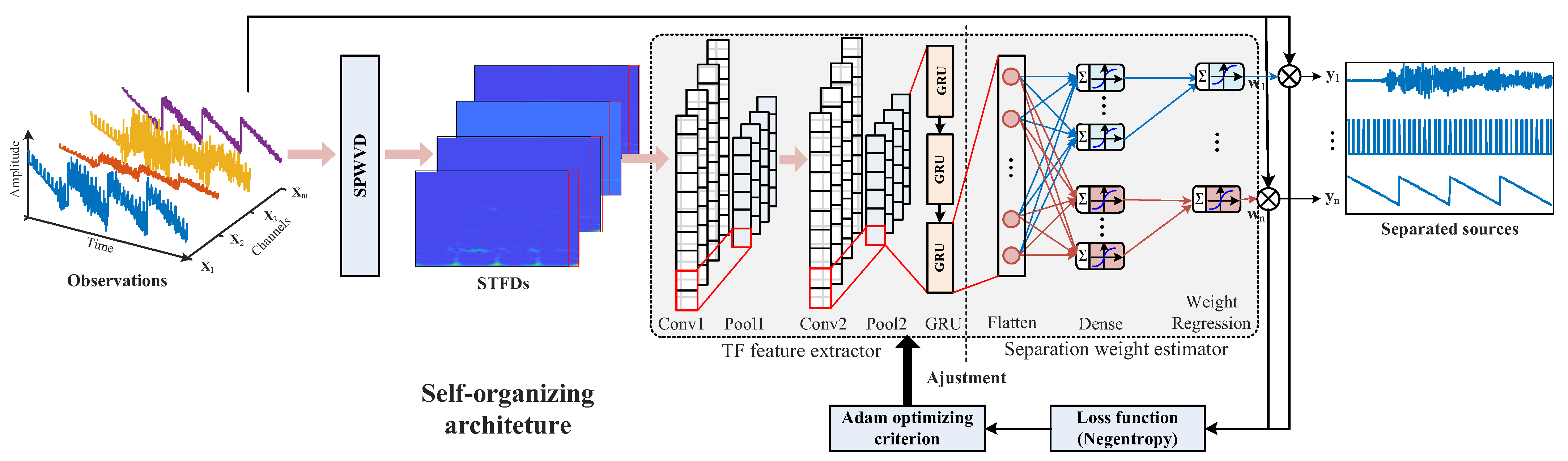
2.3. Enhanced Defect Detection with a Time–Frequency Separation Neural Network

As shown in Figure 2, a time–frequency separation neural network (TFSNN) was proposed on the basis of an instantaneous mixing scenario in order to separate the independent acoustic source and identify the AE defect signal. The topological structure of TFSNN mainly includes two parts, a TF feature extractor and a separation weight estimator. Notably, estimating the separation sources or weights is the ultimate aim in such a self-organizing structure. The training process of this network is also the estimating process of the final separation weights. In this sense, the output of this network is specified for a certain mixing system or weights, and the network should be retrained if the mixing system changes. In addition, the whole-length mixture observations are the only data provided to the network, which can be regarded as both training and testing datasets. Given a set of mixture observations, $x(t)=\left[x_1(t),\cdots ,x_m(t)\right]$, the signals should first be centralized (subtracting their mean) and pre-whitened to guarantee the uncorrelated hypothesis just as the conventional ICA theorem requires. According to authors’ previous work, the pre-whitening process could be easily achieved through singular value decomposition (SVD) or Schmidt orthogonalization of the observations’ autocorrelation matrix [11]. Then, the pre-whitened signals are transformed into spatial time–frequency distributions (STFDs), using SPWVD to obtain a high-resolution representation in both the time and frequency domains. Subsequently, following the temporal order, the frequency spectrum in the STFDs is successively fed into the feature extractor of the network in a frame-by-frame manner.

2.3.1. TF Feature Extractor

The TF feature extractor is actually shared among the weight estimators in different channels. The first four layers of the feature extractor are composed of two stacked one-dimensional convolutional neural network (1D-CNN) layers and two max pooling layers, which are used to extract the dominant spectrum characteristics of a single time-frame in the input STFD spectrogram.

A one-dimensional convolutional neural network is a well-known local connectivity architecture characterized by its filter kernels and activation functions. The computing process of an lth-layer 1D-CNN is described as follows:

$$a_k^l={\delta }_l\left(b_k^l+{\displaystyle \sum _{i=1,i\in M_l}^{N_{l-1}}{w}_{ik}^l\ast }{a}_i^{l-1}\right)$$

(7)

Where $M_l$ is the set of filter kernels in the lth-layer, and $w_k^l,b_k^l$ are the weights and bias for the kth kernel, respectively. $a^{l-1}$ is the l-1th-layer output and lth-layer input. “$\ast$” denotes the convolution operator. ${\delta }_l$ is the activation function to perform a nonlinear transformation, adopted as tangent or ReLU (rectified linear unit) in this paper. A max pooling layer is added subsequently for dimension reduction of the features. After these successive operations, the spectrum features in time frame t₀, $STFD\left(t_0,f\right)$, can be significantly compressed, and the dominant features of the AE are automatically selected by the extractor in an end-to-end manner. They are used in the sequential modeling for the next step.

To capture the inherent dependency of the sequential spectrogram, a gated recurrent unit (GRU) layer is employed after 1D-CNN layers. A GRU is an improved and expedited version of a recurrent neural network (RNN), which overcomes the time gradient explosion problem in conventional RNNs through designed gates and converges faster than the long short-term memory (LSTM) network through positive structural simplification [27]. The general mechanism of a GRU layer is controlled by two gates, update gate ${\mathbf{z}}_t$ and reset gate ${\mathbf{r}}_t$, whose formula is shown below.

$$\left\{\begin{array}{l}{\tilde{\mathbf{h}}}_t=\delta \left({\mathbf{W}}_h\cdot \left[{\mathbf{r}}_t\ast {\mathbf{h}}_{t-1},{\mathbf{a}}_t\right]+{\mathbf{b}}_h\right)\\ {\mathbf{h}}_t=\left(1-{\mathbf{z}}_t\right)\odot {\mathbf{h}}_{t-1}+{\mathbf{z}}_t\odot {\tilde{\mathbf{h}}}_t\\ {\mathbf{z}}_t=\sigma \left({\mathbf{W}}_z\cdot \left[{\mathbf{h}}_{t-1},{\mathbf{a}}_t\right]+{\mathbf{b}}_z\right)\\ {\mathbf{r}}_t=\sigma \left({\mathbf{W}}_r\cdot \left[{\mathbf{h}}_{t-1},{\mathbf{a}}_t\right]+{\mathbf{b}}_r\right)\end{array}\right.$$

(8)

where ${\mathbf{a}}_t,{\tilde{\mathbf{h}}}_t,{\mathbf{h}}_t$ denote the input, memory state, and output in the time frame t. ${\mathbf{W}}_{\mu }$ and ${\mathbf{b}}_{\mu }$ imply the weights and biases in the gates; $\mu =h,r,z$. $\sigma$ is the sigmoid function, and “$\odot$” is the element-wise multiplying operator. The memory state, ${\tilde{\mathbf{h}}}_t$, is updated in accordance with ${\mathbf{z}}_t$, and ${\mathbf{r}}_t$ decides if the historical state should be forgotten. In this way, the correlation between frequency characteristics in different time frames can be accurately modelled and gives a better understanding of the above-mentioned spatial time–frequency distributions.

2.3.2. Separation Weight Estimator and Loss Function

After extracting the high-level time–frequency features, the separation weights of the features can be acquired from a dense or fully-connected layer regressor. The dense layers can be divided into n modules, with each module estimating the separation weight for an individual source. The output of the ith module is a 1 × m vector, w_i. When multiplied with the original observation signals, the separated sources can be attained and used to calculate the objective function with the separation weights as follows:

$$\begin{array}{l}\mathcal{l}\left(W\right)=-{\displaystyle \frac{1}{L}}{\displaystyle \sum _{i=1}^n{\displaystyle \sum _{t=1}^L{\left[G\left(y_{Gauss}\right)-G\left(y_i\left(t\right)\right)\right]}^2}}+\lambda {\mathcal{l}}_2\left(W\right)\\ =-{\displaystyle \frac{1}{L}}{\displaystyle \sum _{i=1}^n{\displaystyle \sum _{t=1}^L{\left[g_{Gauss}^i-G\left(w_{i}x\left(t\right)\right)\right]}^2}+\frac{\lambda }{L}{‖W‖}_2^2}\end{array}$$

(9)

where n, L indicates the number of sources and sampling points in the signal, respectively. $\lambda$ is the adjustment coefficient to balance the two losses. $g_{Gauss}$ is a constant related to the Gaussian distribution, which is determined only if the observation signals remain invariant. The objective or loss function of the network comprises two parts in Equation (9), namely the non-Gaussianity and L2 regularization part. The negative non-Gaussianity loss was calculated with the third approximate function for negentropy, generated from the CDF of the super Gaussian distribution in Section 2.1, of which the local minimum revealed a potential candidate of an independent source. The L2 regularization term is added as a penalty term to improve the sparsity and further prevent overfitting in the optimization. Moreover, since the objective and optimization mechanism in networks are quite independent from each other, the proposed method can be combined with lots of superior optimizers to obtain a more accurate separation performance, such as with stochastic gradient descent, Levenberg, RMSprop, Adagrad, and adaptive moment estimation (Adam) [28]. The Adam optimizing criterion was selected in this study in view of its advantages in adaptive learning rates, fast convergence, and highly efficient computation.

In summary, the estimation of separation weights is essentially a regression task. Unlike traditional regression networks, the target in this self-organizing task is not a preset sequence but is determined by the extreme value in the non-negentropy criterion. In light of the proposed structure, the separation weights could be estimated accurately with sufficient training of the observation signals.

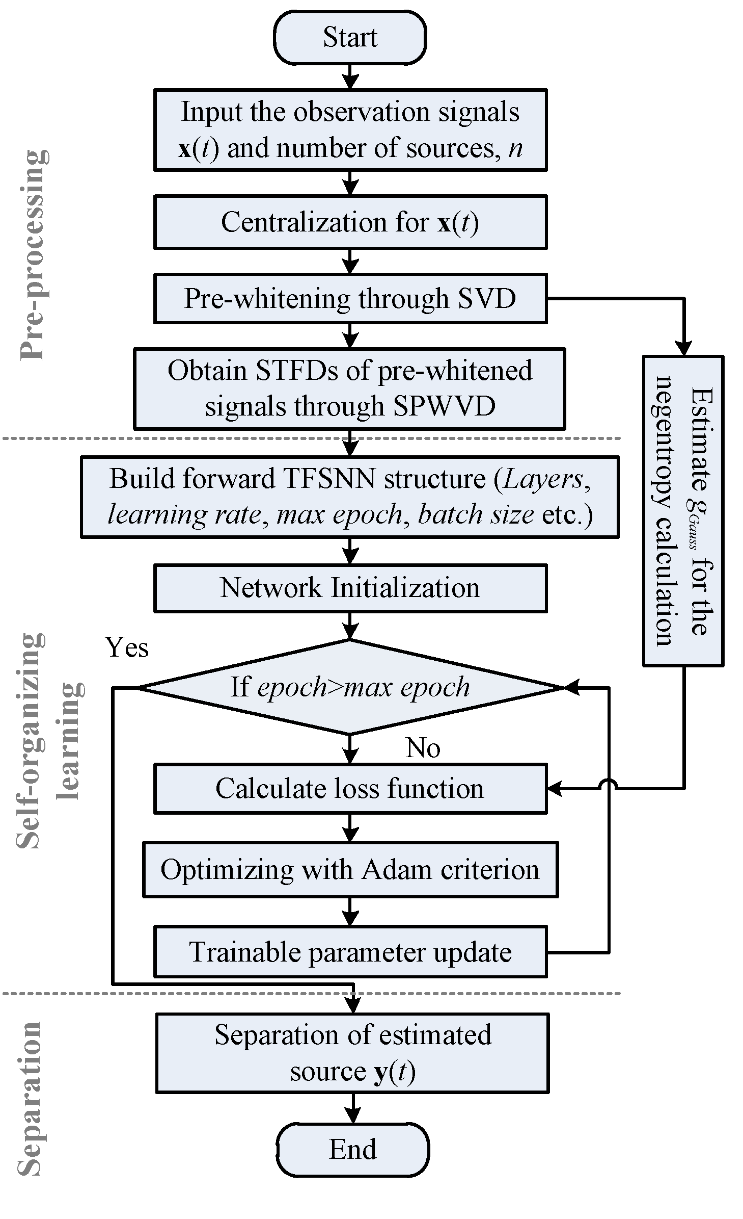
2.3.3. Overall Procedure of the Proposed TFSNN Method

After defining the forward structure and training options of the TFSNN, such as layers, neurons, learning rate, optimizer criterion, etc., the flow chart of the TFSNN employed in separation of AE defect signals is shown in Figure 3. Note that the true source number, n, should be first given in this analysis. The entire procedure can be divided into the following three main steps: (1) pre-processing of the observations, (2) self-organizing or adaptive learning of the trainable network parameters, and (3) separation of the estimated sources after the network is trained. Detailed operations for the main steps are shown in the flow chart. Theoretically, the proposed method has the following advantages or novelties in the source separation task:

• Precise representation of the time–frequency spectrogram for the mixture signals. Firstly, a superior time–frequency analysis, namely SPWVD, is combined as a pre-processing technique. SPWVD is an improved version of TFA, which can both suppress the cross-item interference and retain a high-resolution spectrogram. In this way, the characteristics of sources can be represented in a more accurate manner.
• Sufficient exploitation of the inherent time–frequency characteristics for the AE signals: To cooperate with the STFDs, 1D-CNN and GRU structures were introduced in the TFSNN to extract and exploit the dominant characteristics from AE signals’ TF representation.
• High accuracy and stable acquisition of the separation weights with the self-organizing network: The above learned features were provided to the separation regressor, and the optimization process can be achieved using powerful network optimizers such as Adam rather than a traditional quasi-Newton method. Hence, it can avoid oscillation and provide a faster convergence and higher accuracy.

In summary, combined with the adaptive separation network, it promises outstanding performance in the separation and extraction of impulsive rail defect signals. The proposed method will be utilized and subsequently compared with the typical BSS methods in the source separation of simulation and experimental railway AE signals. The mentioned superiorities of the proposed method will also be verified in detail.

3. Experiments and Datasets

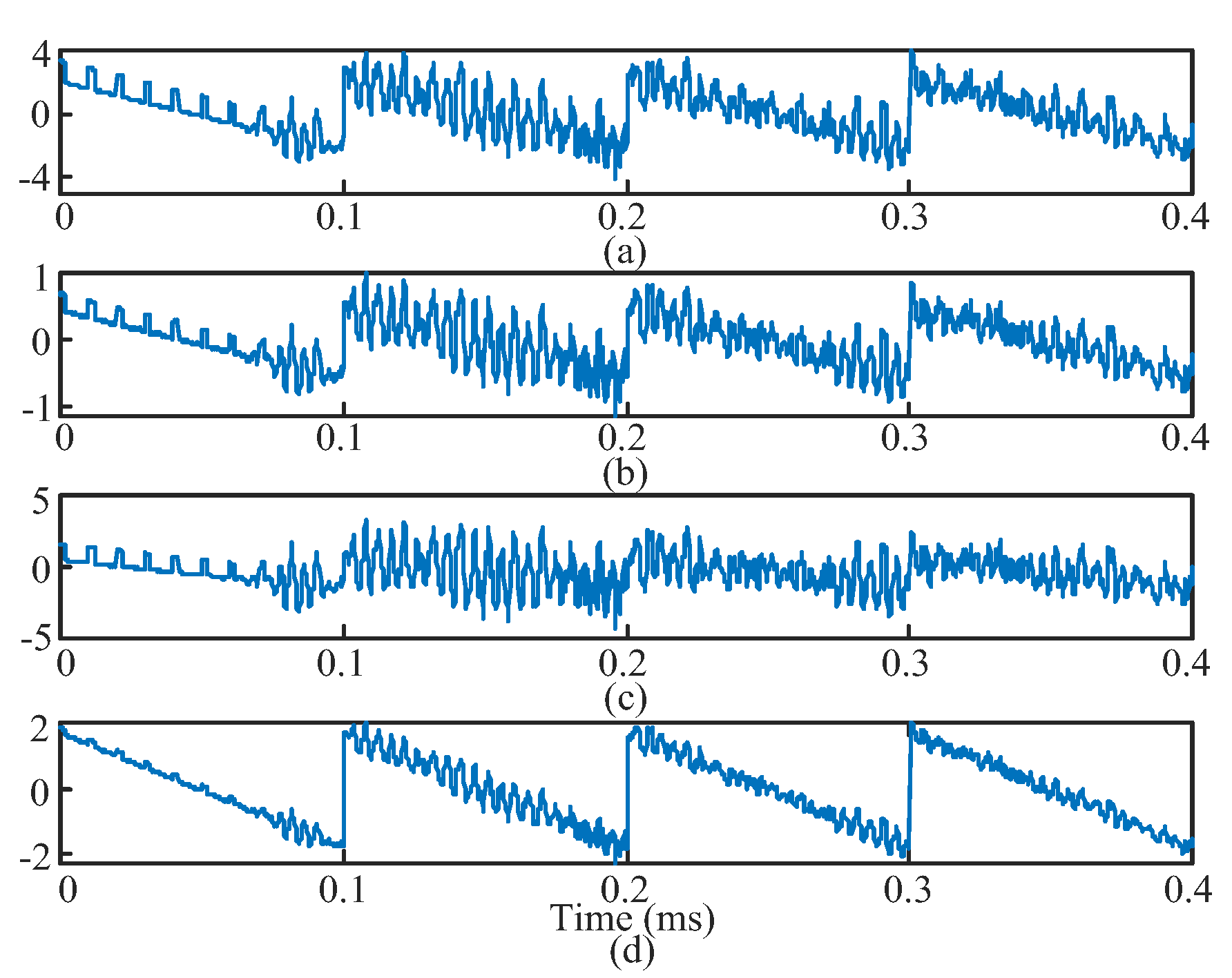
3.1. Case 1: Validation with Generated Interferences and Four-Channel Simulations

The signals used in the algorithm validations include the following two types: Case 1, separation of rail cracks under simulated noise interference, and Case 2, Separation of rail cracks under real additive railway noise. The simulation validation (Case 1) was used to make sure the feasibility of the proposed method in a standard separation task with a specific known source number. The experimental validation (Case 2) was used to verify the applicability of the proposed method in an actual railway environment. The proposed method is first compared with different BSS methods in a three-source and four-channel simulation. In the simulated experiment, the actual burst-type rail crack signal is adopted as the investigated signal. These actual crack signals were previously acquired in tensile tests of a rail specimen [29]. A detailed description of the tensile test system has been given previously and will not be repeated here. To match the actual crack signal, the sampling rates of the source signals are all 5 MHz with a length of 0.4 ms. The ramp waves and square pulses represent the periodic and impulse interference signals, which normally exist in a typical railway analysis. The frequency of the ramp wave is 10 kHz, while the frequency of square pulse is 100 kHz with a 20 percent duty cycle. The original sources are shown in Figure 4.

To simulate the signals received by a sensor array and compare the methods under the same conditions, for the simulation the four source signals are mixed using an arbitrarily chosen mixing matrix in Equation (10).

$$A=\left[\begin{array}{c}\begin{array}{ccc}0.545& 0.588& 0.993\end{array}\\ \begin{array}{ccc}0.172& 0.121& 0.253\end{array}\\ \begin{array}{ccc}0.853& 0.554& 0.533\end{array}\\ \begin{array}{ccc}0.180& 0.082& 0.892\end{array}\end{array}\right]$$

(10)

Furthermore, a uniformly-distributed random noise, which has a −20 dB amplitude level against the noise-free observation, is added to all channels of mixtures to testify to the robustness against noise interference, and the final observed signals of this simulation are shown in Figure 5.

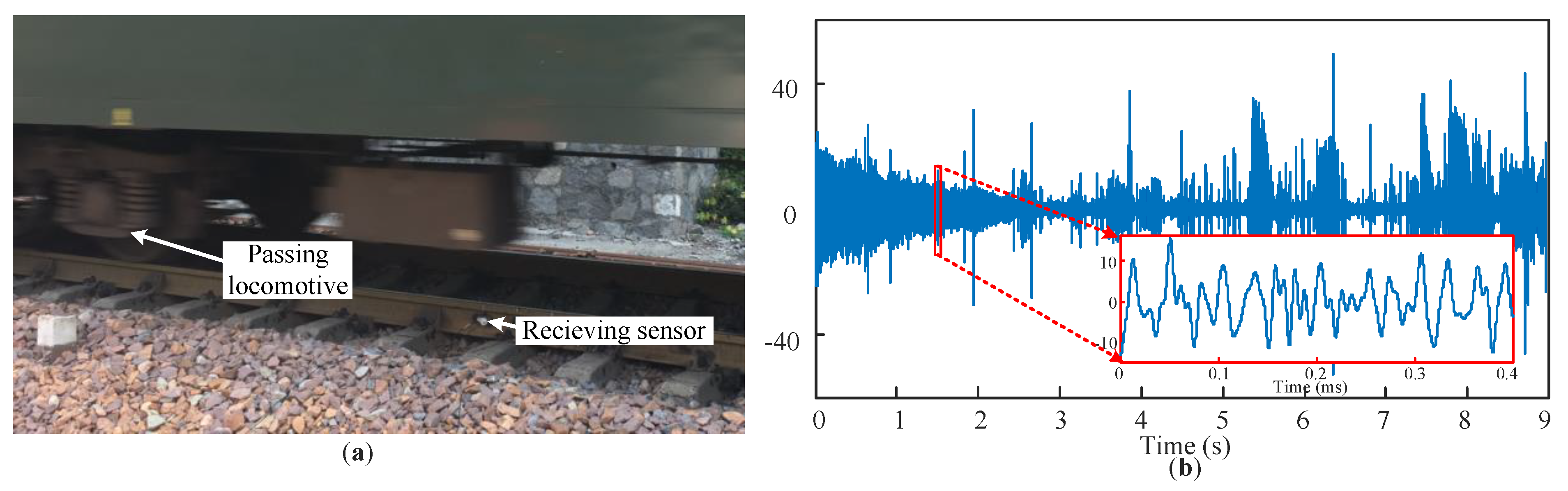
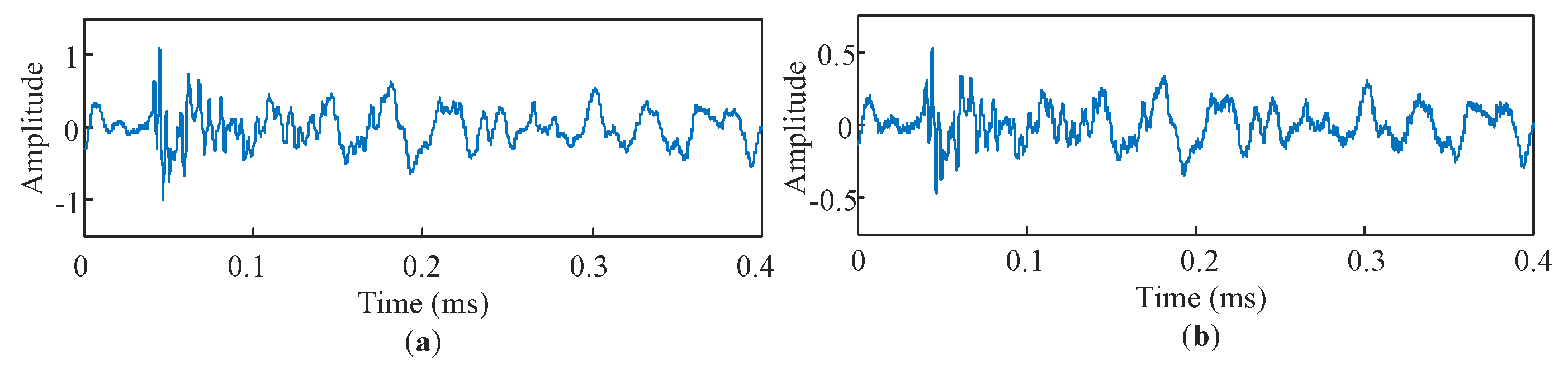
3.2. Case 2: Validation with Rail Crack Signals and Actual Additive Railway Noises

In order to investigate the proposed method in real operating conditions, AE wheel–rail noise signals were acquired from an actual rail line in Jiaozuo, Henan province [30]. The rail tracks were made up of 60 kg/m rails and the material U75V. The tracks were examined to ensure they were intact in advance. As is shown in Figure 6a, the experiment is carried out when a passenger train is passing. The speed of the passenger locomotive is about 55 km/h. The sensor was fixed on the rail waist by the mechanical clamp, and couplant was used to fill between the sensor and rail surface for better signal transmissibility.

AE signals were obtained through the acquisition system with a sampling rate of 5 MHz (Model: Vallen AMSY-6 ASIP-2/A; Vallen Systeme GmbH; Wolfratshausen, Germany). One receiving sensor is attached to the rail waist with a wideband of 100–900 kHz (Model: PAC WSα; Mistras Group, Inc.; Princeton Junction, NJ, USA). The signals were continuously collected under the interference of a variety of real noises caused by wheel–rail contact movements. An example of 9 s of continuous, pure, actual railway noise is shown in Figure 6b, and the noise test sets with 100 test noise samples were randomly selected and truncated from the raw continuous noise signal, as shown in the subfigure. Each sample was truncated to a length of 0.4 ms and used to generated synthetized noisy signals with 100 random AE crack signals for a systematic evaluation of the different methods. In on-site railways, the AE noise components are typically complex. In practice, noise signals comprise both stationary/periodic noise and non-stationary/impulsive noise [31]. The stationary noise is generally attributed to normal wheel–rail interactions, such as rolling contacts. In contrast, impulsive noise arises from abnormal interactions, such as braking, impacts, and severe friction, often exhibiting characteristics in the high-frequency band and even overlapping with the defect spectrum.

Using the smoothed pseudo Wigner–Ville distribution for time–frequency transformation, the spatial time–frequency distributions of an exemplified rail crack signal, periodic, and abnormal noise signals from the datasets are shown in Figure 7. A typical observation mixture of the actual signals, composed of the sources in Figure 7, is shown in Figure 8. In Figure 7a, the rail crack signal exhibits a non-stationary, wideband characteristic, and the dominant component of actual railway noise shows a relatively low-frequency characteristic. Moreover, as shown in Figure 7c, there also exists some unpredictable short-term abnormal impulsive noise, which also has an obvious non-stationary characteristic and overlap band with the defect signals, further hindering the separation with typical linear filters. Therefore, the overall separation performance will be illustrated later.

4. Results

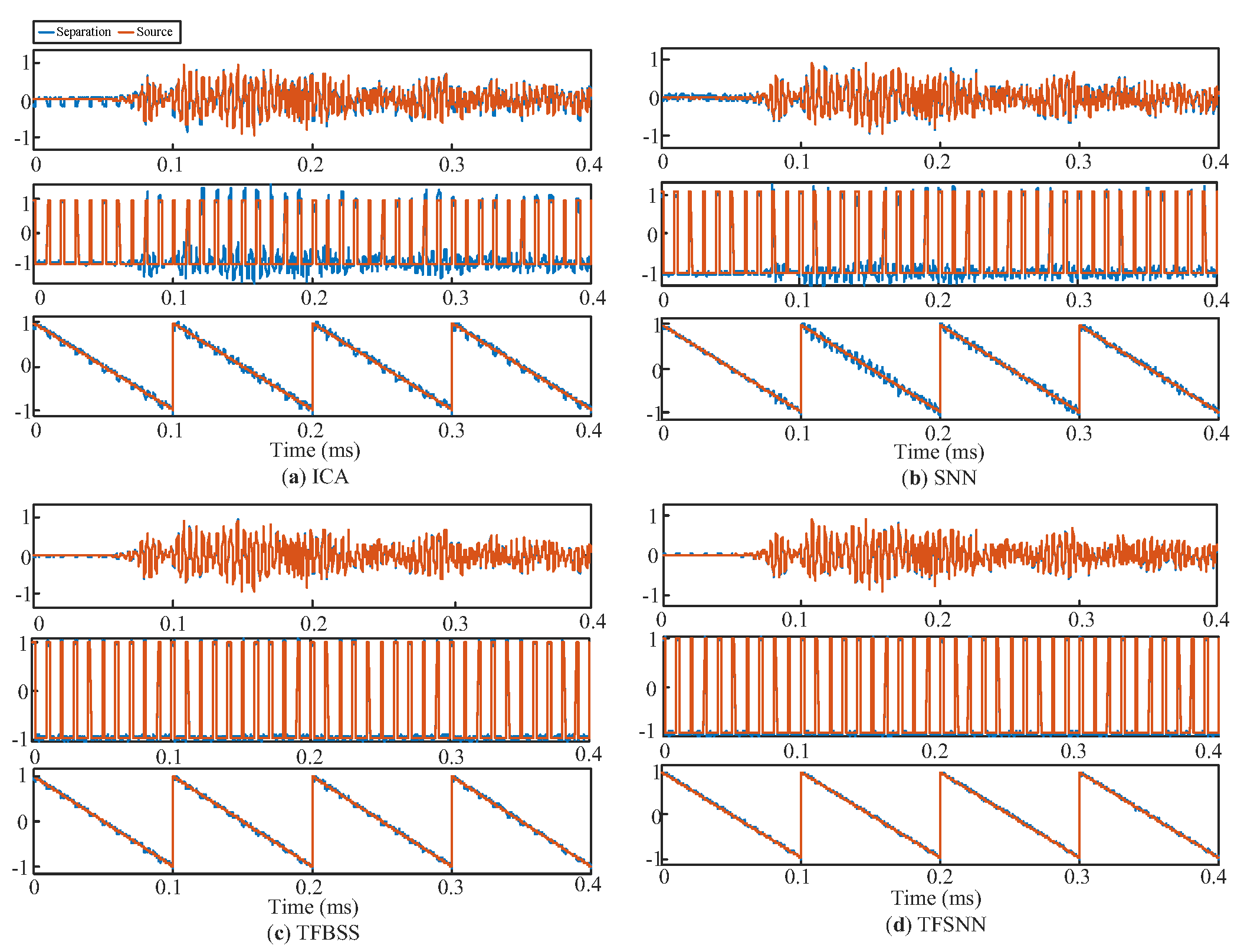
4.1. Defect Separation Performance with Simulated Test Signals

The defect separation performance in Case 1 is first analyzed with the simulated mixture signals. To validate the superiority of the TFSNN, in this section it was compared with the representative methods of ICA [7], a fully-connected shallow neural network (SNN) [14], and TFBSS [22]. The separated signals and original source signals are shown in Figure 9. To visualize them on the same scale, the separated signals were Z-score standardized to ensure they have the same mean and variance as the corresponding sources. From the visual results, it can be intuitively seen that the proposed method significantly outperformed the other three algorithms in separating the crack signal, the ramp, and the square wave signals. Particularly, the recovered details of the ramp and defect signals were difficult to distinguish in ICA and SNN. Due to a lack of TF exploitation, both ICA and SNN seemed to suffer more seriously from the interference non-stationary crack signal. Next, we evaluate the separation effects of the above algorithms horizontally using two evaluation criteria, a scale-invariant signal-to-noise ratio and a similarity coefficient.

Considering the scale ambiguity for BSS, the classical signal-to-noise ratio (SNR), referring to the ratio of power between the target source signal and the residual error, is recently proved inaccurate or misleading in BSS tasks [32]. An improved version of SNR, scale-invariant signal-to-noise ratio (SISNR), measures the level of distortion or noise interference in a processed signal by comparing it to a reference signal in a way that is invariant to the scaling of the signals [33]. This metric is useful for evaluating speech enhancement and source separation by eliminating the scale ambiguity and ensuring that the residual errors are indeed orthogonal or uncorrelated to the target. Therefore, SISNR is selected as the first evaluation metric in this paper. SISNR is calculated according to the following formula, where s is the reference signal and ŝ is the separated or processed signal:

$$SISN{R}_i=10\lg {\displaystyle \frac{{‖\alpha s_i^2(t)‖}^2}{‖\alpha s_i^2(t)-{\widehat{s}}_i^2(t)‖}}$$

(11)

where $\alpha ={\widehat{s}}^{T}s/{‖s‖}^2$. A higher SISNR value indicates a lower level of the noise signal, implying a better separation effect of the blind signal separation algorithm. The SISNRs for different separated signals in Figure 8 are listed in

Table 1. SISNRs (dB) of blind separated signals using different methods.

Algorithm	Crack	Square Pulse	Ramp
ICA	10.6537	12.5581	20.1588
SNN	15.3378	13.4418	20.7815
TFBSS	24.0757	29.3030	25.0376
TFSNN	26.5158	32.2905	28.2357

.

On the one hand, the SISNRs clearly indicated that both of the TFA-based methods could suppress the residual noise to a much lower level than the pure time-domain methods, hence providing an over 10 dB increment in averaged SISNR. In particular, the proposed method further exhibited a 2.87 dB higher SISNR than the classical TFBSS, which verified the necessity and efficiency of applying network optimization. On the other hand, the similarity coefficient between the source and separated signals is calculated as follows:

$${\delta }_i=\delta ({\widehat{s}}_i,s_i)={\displaystyle \frac{{\displaystyle \sum _{t=1}^L{\widehat{s}}_i(t)s_i(t)}}{\sqrt{{\displaystyle \sum _{t=1}^L{\widehat{s}}_i^2(t)}{\displaystyle \sum _{t=1}^L{s}_i^2(t)}}}}$$

(12)

The similarity coefficient indicates the degree of waveform similarity between the separated signal and the source signal, overcoming the uncertainty caused by source separation, serving as a measure to evaluate the quality of the TF characteristic and detail recovery in BSS. A coefficient closer to 1 indicates that the waveform of the ith separated signal is closer to that of the ith source signal, thus indicating a better preservation of the TF characteristics for the original sources. The similarity coefficients for different separated signals in Figure 8 are listed in

Table 2. Similarity coefficients between separated signals and sources using different methods.

Algorithm	Crack	Square Pulse	Ramp
ICA	0.9470	0.9723	0.9952
SNN	0.9854	0.9947	0.9958
TFBSS	0.9980	0.9994	0.9984
TFSNN	0.9982	0.9997	0.9992

. In accordance with SISNRs, the similarity coefficients implied that TFSNN recovered most of the details in the original sources.

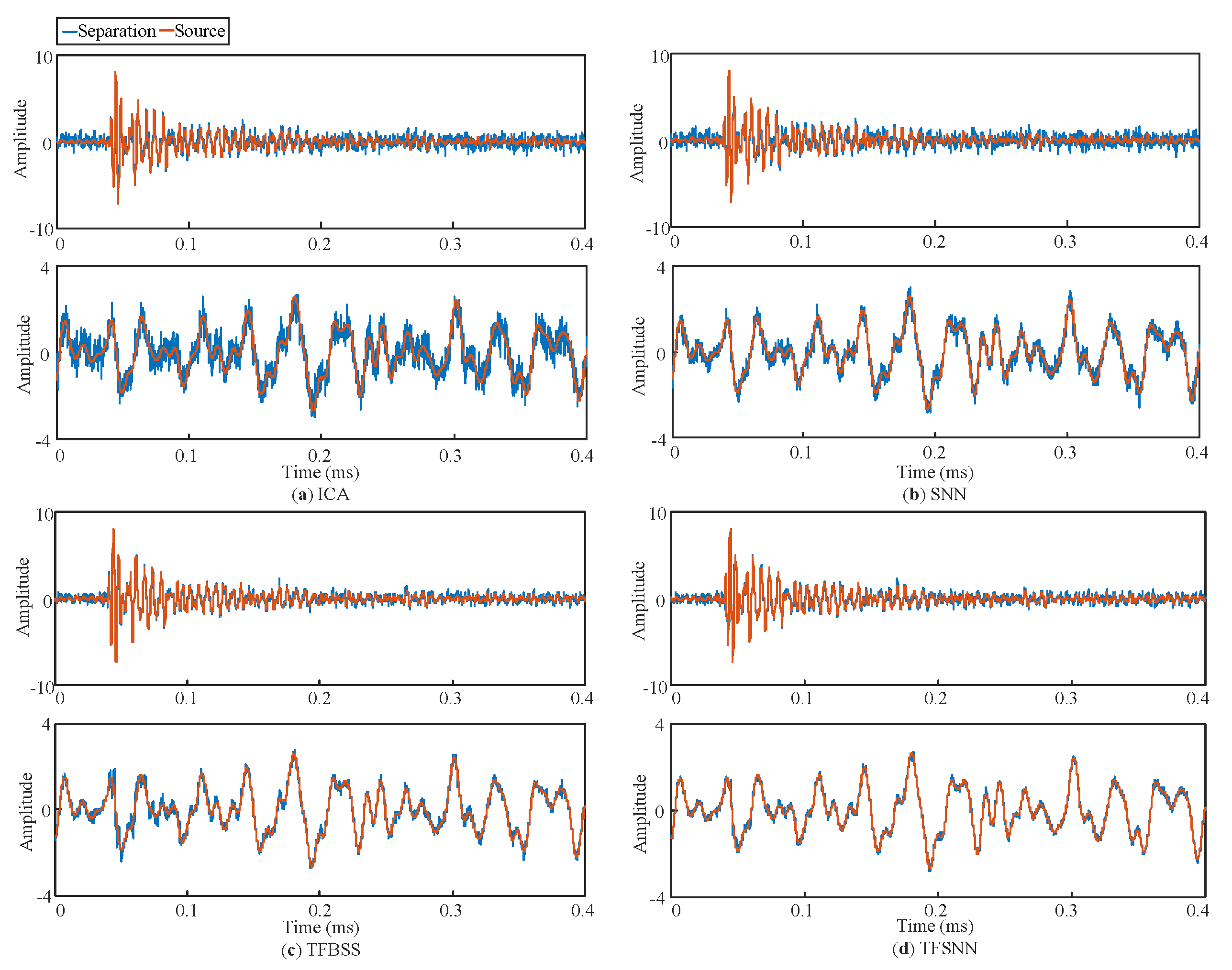
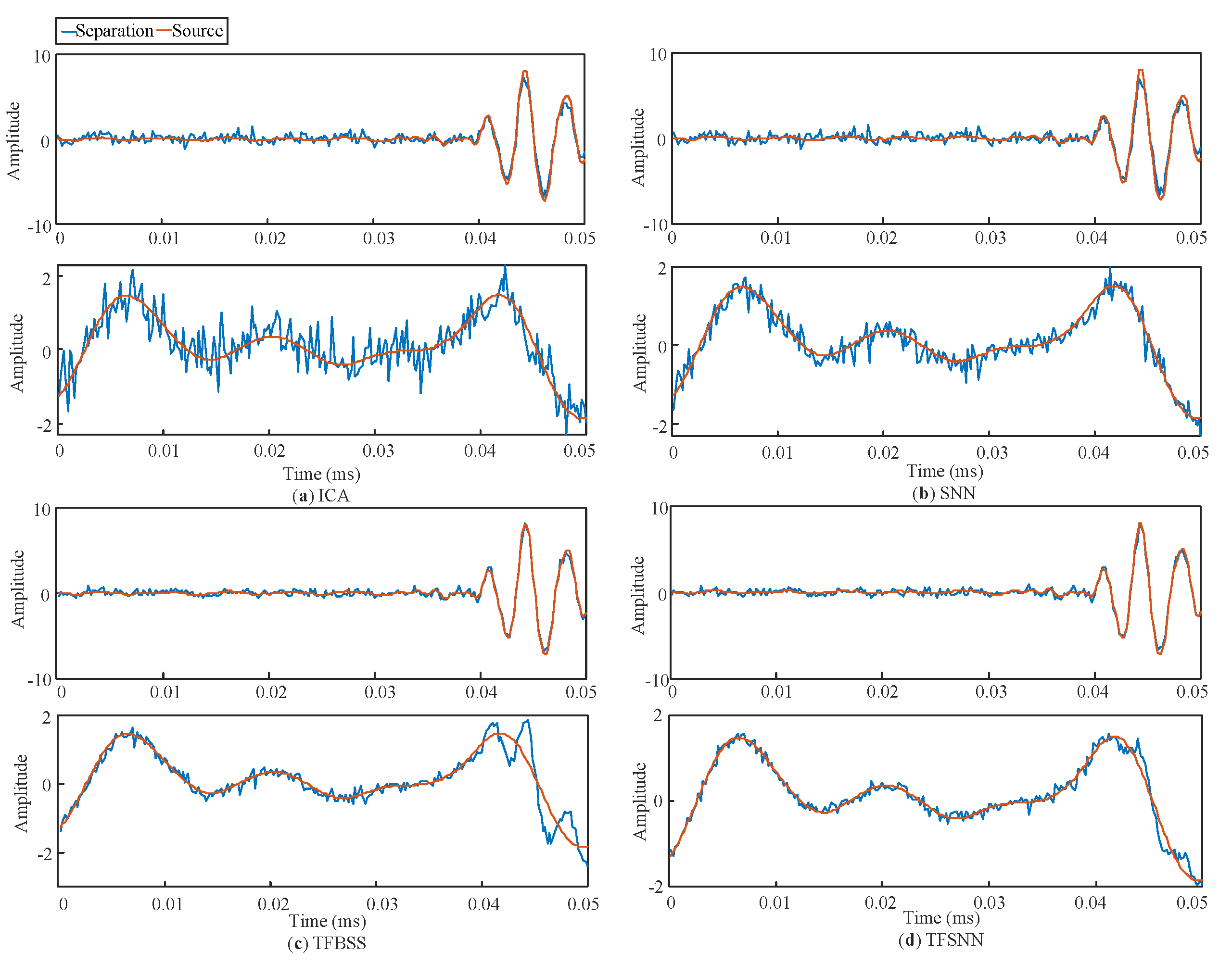
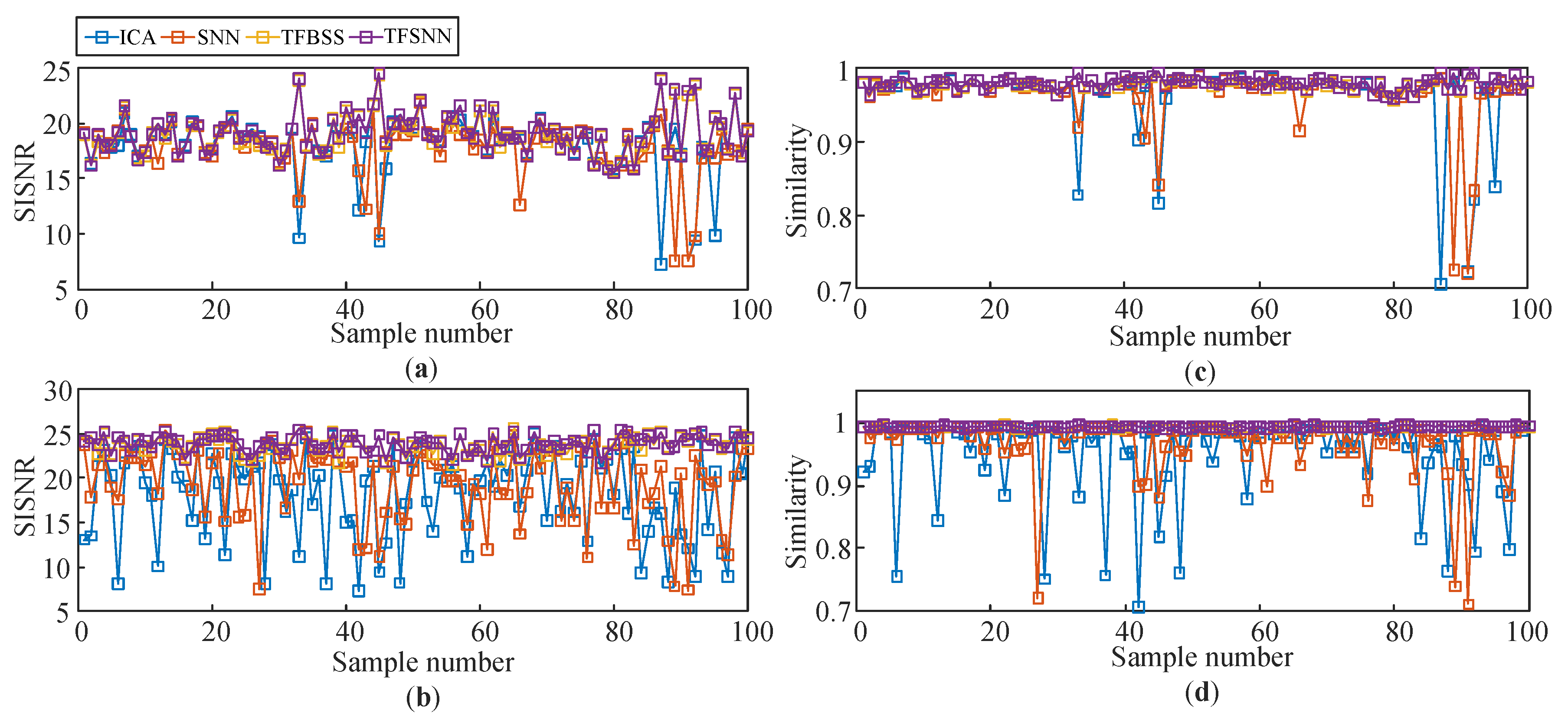
4.2. Defect Separation Performance with Experimentally Acquired Railway Noise Signals

To further validate the practicability of the proposed method for the defect separation, on-site experimental noise is used to represent complicated noise properties and synthetize the two-channel observation signals. Gaussian noises at −20 dB were also added to the observations for the noise resistance investigation. The entire separated signals and a zoomed-in figure of the detailed sections within [0, 0.05] milliseconds are shown in Figure 10 and Figure 11, respectively.

Overall, as shown in Figure 10, the proposed method finds the most accurate projection vector for separation and delivers the best recovery performance. Nevertheless, the separation performances in ICA and SNN are relatively poor, significantly affected by the residual Gaussian noise and abnormal railway noise. The noises with obvious amplitudes still exist in the extracted crack signal. After Z-score standardization, the root mean square (RMS) of the averaged residual noise in ICA from Figure 10a was 0.3882, approximately three times higher than the RMS of the residuals in TFBSS at 0.1075 and TFSNN at 0.1029. The RMS of the residuals in the SNN was 0.151, also reflecting a significant increase. This suggests that the robustness of ICA and SNN against Gaussian noise is lower compared to the time–frequency domain methods. Particularly, ICA is based on the assumption of pure Gaussianity in the time domain, which may result in its reduced robustness against random Gaussian noise interference and restrain its further application in practice. In contrast, some pulse abnormal noise with minor amplitude still exists in the extracted crack signal of the TFBSS result. Compared to the three algorithms, the proposed method is clearly more effective in detecting rail crack signals in real noise environments, accurately recovering the occurrence of crack signals from noisy mixtures in practice. Even though this is a promising result, it still needs to be systematically compared using an entire group of 100 test signals to further analyze the stability and give a comprehensive conclusion.

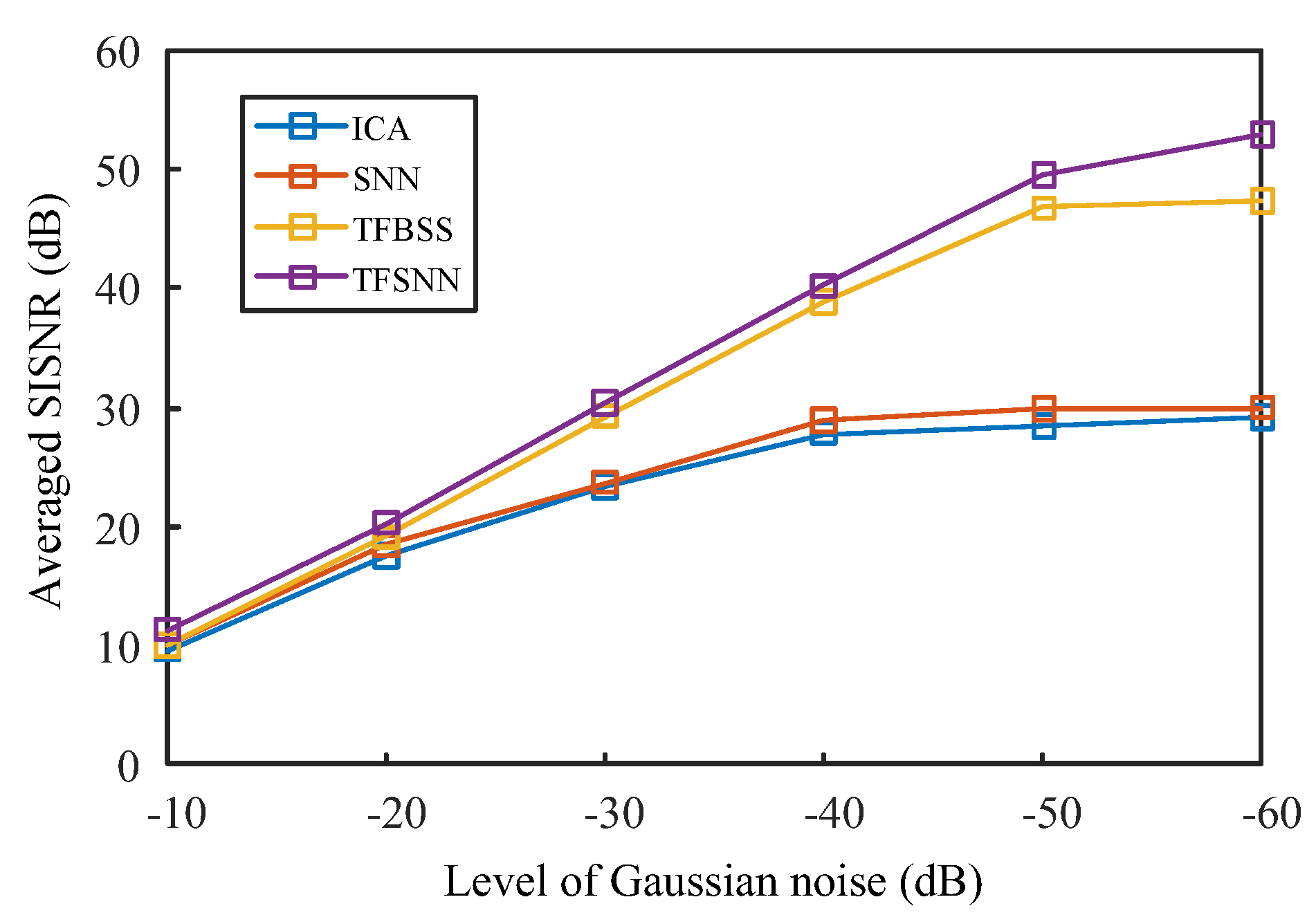
4.3. Systematic Assessment of Comparative Methods with Test Sets and Stability Discussion

On the basis of systematic assessment with the whole test sets in Case 2, the SISNRs for a group of 100 randomly selected test signals are first displayed in Figure 12a,b. The similarity coefficients for the same test group are displayed in Figure 12c,d. In addition, the averaged values and standard deviations of the group SISNRs and group similarity are listed in

Table 3. Averaged SISNR and similarity for the separated sources in a test group of 100 signals.

Algorithm	Averaged SISNR		Averaged Similarity
	Defect	Railway Noise	Defect	Railway Noise
ICA	18.0983 ± 2.8019	18.2298 ± 5.0321	0.9657 ± 0.048	0.9509 ± 0.0678
SNN	17.8321 ± 2.4989	19.5157 ± 4.302	0.9663 ± 0.0419	0.9673 ± 0.0513
TFBSS	18.9886 ± 1.8957	23.7881 ± 1.0311	0.9784 ± 0.008	0.9832 ± 0.0017
TFSNN	19.1102 ± 1.8263	23.9424 ± 0.9326	0.9796 ± 0.007	0.9935 ± 0.0014

.

As stated earlier, the similarity investigates the degree of resemblance between the separated signal and the source signal, reflecting how well the separation retains the details of the source signal. The SISNR assesses the extent of noise suppression during separation based on Equation (11).

From Figure 12c, in the separation of crack signals, most of the similarity coefficients can reach above 0.95. The stability of the separation exhibited varying degrees in different methods, and this point is extremely obvious in several cases when the similarity coefficient abruptly decreased. In contrast, the separation of noise signals produced far more chaotic results. The variance of ICA was the highest, indicating the lowest averaged metrics and a minimal separation stability, while the averaged similarity level and variance of SNN and TFBSS were quite close, and both were inferior to the proposed method. It demonstrated that the proposed method could efficiently recover more time–frequency details of the sources in most separation processes.

The overall and averaged SISNRs for the crack and noise signals are shown in Figure 12a,b. In terms of SISNR, the four algorithms show significant differences in noise suppression effects. All the compared methods can provide roughly satisfactory separation results, with 15 dB for defect signals. While for railway noise signal separation, the ICA and SNN algorithms were significantly weaker (about 5 dB lower) than the TFA-based algorithms, and the separated signals were still interfered with by the residual abnormal noises. Moreover, the dynamic robustness of the compared methods against different Gaussian noise levels was evaluated, as shown in Figure 13. As the noise amplitude decreased from −10 dB to −60 dB, the compared methods gradually converged and reached their maximal SISNRs, where TFSNN obtained an approximately 20 dB higher SISNR than the time domain methods and 5 dB higher than TFBSS. This indicated the separation accuracy or convergence limits of the time–frequency methods were much higher than the time domain methods. When the noise amplitude increased to −10 dB, all the compared methods degraded significantly. However, the proposed method degraded at a much lower speed and remained about 2 dB higher than the compared methods in this case. This indicated a better robustness of the proposed method under random noise interferences.

In conclusion, as shown in Figure 12 and Table 3, the performance of different BSS methods is mainly influenced by their stability. For an easy and stationary separation case, the four algorithms might provide a basically identical separation performance. In challenging separation scenarios like non-stationary noise, the absence of time–frequency (TF) analysis can cause traditional algorithms to experience significant degradation, resulting in a decreased average separation performance. Theoretically, time domain BSS methods such as ICA assume statistical independence in either the time or frequency domain. However, this assumption may not hold for non-stationary signals, where the frequency content varies with time, and it makes the methods sensitive to the signals [34]. Particularly, in a noisy environment characterized by time-varying frequency content, the adaptive tracking capabilities of time domain BSS might become unstable, potentially leading to degraded separation performance due to violation of the fundamental assumption. This result is substantiated in Figure 12. Then, averaged performance of the whole test sets was determined by the proportion of degraded samples. A lower instability for ICA and SNN made for a higher possibility of degradation, while time–frequency BSS is particularly useful in this case, taking full advantage of the time–frequency information.

5. Conclusions

In this paper, a rail defect signal extraction method based on a time–frequency separation neural network is proposed. Firstly, a superior time–frequency analysis, namely SPWVD, is combined as a pre-processing technique to retain a high-resolution spectrogram. Then, a specific structure including a 1D-CNN feature extractor and a weight estimator was utilized to avoid oscillation and provide a faster convergence and higher accuracy. In this way, the proposed TFSNN is expected to greatly improve separation efficiency and recovery details. Compared with the separation effect of three classical BSS algorithms, the simulation and experimental results show that the separation effect of the improved algorithm is superior to the others in most cases, which verifies the necessity and advantages of integrating TF analysis and adaptive self-organizing neural networks into BSS problems. In its results, this research has the potential to offer valuable insights for similar safety and health monitoring applications. Although TFSNN offers promising solutions to address key challenges in blind source separation (BSS) tasks, such as handling non-stationary signals and improving stability, the noise data utilized in the simulation experiment presented in this paper were collected from a passenger vehicle operating at a maximum speed of approximately 55 km/h. The current experimental validations have not yet accounted for the impact of high-speed railway noise, which typically exhibits broader bandwidth and higher amplitude. To enhance TFSNN’s effectiveness in high-speed and complex noisy environments, further research should focus on integrating joint optimization with flexible separation approaches, such as spectrogram masking, permutation invariant training (PIT), and scale-invariant signal-to-distortion ratios. Also, it is important to modify the TFSNN to be lightweight and scalable, allowing it to handle varying numbers of sources and changing environmental conditions without significant reconfiguration. In this way, it will be more effective and reliable for real-time applications and could be extended to a wider range of real-world scenarios in the future.

References

1. Alahakoon, S.; Sun, Y.; Spiryagin, M.; Cole, C. Rail flaw detection technology for safer, reliable transportation: A review. J. Dyn. Syst. Meas. Control 2018, 140, 020801. [Google Scholar]
2. Wang, K.; Zhang, X.; Song, S.; Wang, Y.; Shen, Y.; Wilcox, P.D. Rail Steel Health Analysis Based on a Novel Genetic Density-based Clustering Technique and Manifold Representation of Acoustic Emission Signals. Appl. Artif. Intell. 2021, 36, 1012–1030. [Google Scholar]
3. Li, Z.R.; Liu, Z.L.; Zuo, M.J. Homotypic multi-source mixed signal decomposition based on maximum time-shift kurtosis for drilling pump fault diagnosis. Mech. Syst. Signal Process. 2024, 221, 111724. [Google Scholar]
4. Gurve, D.; Krishnan, S. Separation of Fetal-ECG Fr om Single-Channel Abdominal ECG Using Activation Scaled Non-Negative Matrix Factorization. IEEE J. Biomed. Health Inform. 2020, 24, 669–680. [Google Scholar]
5. Luo, Z.; Li, C.; Zhu, L. A Comprehensive Survey on Blind Source Separation for Wireless Adaptive Processing: Principles, Perspectives, Challenges and New Research Directions. IEEE Access 2018, 6, 66685–66708. [Google Scholar]
6. Yu, Y.; Wang, W.; Han, P. Localization based stereo speech source separation using probabilistic time-frequency masking and deep neural networks. EURASIP J. Audio Speech Music Process. 2016, 2016, 7. [Google Scholar]
7. Maddirala, A.K.; Shaik, R.A. Separation of Sources from Single-Channel EEG Signals Using Independent Component Analysis. IEEE Trans. Instrum. Meas. 2017, 10, 2775358. [Google Scholar]
8. Mohanaprasad, K.; Singh, A.; Sinha, K.; Ketkar, T. Noise reduction in speech signals using adaptive independent component analysis (ICA) for hands free communication devices. Int. J. Speech Technol. 2019, 22, 169–177. [Google Scholar]
9. Jian, J.; Wang, L.; Lu, Z.R. Enhancing second-order blind identification for underdetermined operational modal analysis through bandlimited source separation. J. Sound Vib. 2024, 572, 118179. [Google Scholar]
10. Chowdhury, J.H.; Shihab, M.; Pramanik, S.K.; Hossain, M.S.; Ferdous, K.; Shahriar, M. Separation of Heartbeat Waveforms of Simultaneous Two-Subjects Using Independent Component Analysis and Empirical Mode Decomposition. IEEE Microw. Wirel. Technol. Lett. 2024, 34, 1059–1062. [Google Scholar]
11. Wang, K.; Hao, Q.; Zhang, X.; Tang, Z.; Wang, Y.; Shen, Y. Blind source extraction of acoustic emission signals for rail cracks based on ensemble empirical mode decomposition and constrained independent component analysis. Measurement 2020, 157, 107653. [Google Scholar]
12. Ansari, S.; Alatrany, A.S.; Alnajjar, K.A.; Khater, T.; Mahmoud, S.; Al-Jumeily, D.; Hussain, A.J. A survey of artificial intelligence approaches in blind source separation. Neurocomputing 2023, 561, 126895. [Google Scholar]
13. Isomura, T.; Tpyoizumi, T. Multi-context blind source separation by error-gated Hebbian rule. Sci. Rep. 2019, 9, 7127. [Google Scholar]
14. Liu, S.; Wang, B.; Zhang, L. Blind Source Separation Method Based on Neural Network with Bias Term and Maximum Likelihood Estimation Criterion. Sensors 2021, 21, 973. [Google Scholar] [CrossRef]
15. Luo, Y.; Mesgarani, N. Conv-TasNet: Surpassing Ideal Time–Frequency Magnitude Masking for Speech Separation. IEEE Trans. Audio Speech Lang. Process. 2019, 27, 1256–1266. [Google Scholar]
16. Sinha, R.; Rollwage, C.; Doclo, S. Variants of LSTM cells for single-channel speaker-conditioned target speaker extraction. EURASIP J. Audio Speech Music Process. 2024, 2024, 16. [Google Scholar]
17. Lee, K.J.; Lee, B. End-to-End Deep Learning Architecture for Separating Maternal and Fetal ECGs Using W-Net. IEEE Access 2022, 10, 39782–39788. [Google Scholar]
18. Li, Y.; Ramli, D.A. Advances in Time-Frequency Analysis for Blind Source Separation: Challenges, Contributions, and Emerging Trends. IEEE Access 2023, 11, 137450–137474. [Google Scholar]
19. Massar, H.; Drissi, T.B.; Nsiri, B.; Miyara, M. Advancements in Blind Source Separation for EEG Artifact Removal: A comparative analysis of Variational Mode Decomposition and Discrete Wavelet Transform approaches. Appl. Acoust. 2025, 228, 110300. [Google Scholar]
20. Cheng, W.; Jia, Z.; Chen, X.; Han, L.; Zhou, G.; Gao, L. Underdetermined convolutive blind source separation in the time–frequency domain based on single source points and experimental validation. Meas. Sci. Technol. 2020, 31, 095001. [Google Scholar]
21. Benkedjouh, T.; Zerhouni, N.; Rechak, S. Tool wear condition monitoring based on continuous wavelet transform and blind source separation. Int. J. Adv. Technol. 2018, 97, 3311–3323. [Google Scholar]
22. Morovati, V.; Kazemi, M.T. Detection of sudden structural damage using blind source separation and time–frequency approaches. Smart Mater. Struct. 2016, 25, 055008. [Google Scholar]
23. Elouaham, S.; Nassiri, B.; Dliou, A.; Zougagh, H.; El Kamoun, N.; El Khadiri, K.; Said, S. Combination time-frequency and empirical wavelet transform methods for removal of composite noise in EMG signals. TELKOMNIKA Telecommun. Comput. Electron. Control 2023, 21, 1373–1381. [Google Scholar]
24. Sun, H.; Fang, L.; Guo, J. A fault feature extraction method for rotating shaft with multiple weak faults based on underdetermined blind source signal. Meas. Sci. Technol. 2018, 29, 125901. [Google Scholar]
25. Liu, J.; Zhang, K.; Wang, Z. Identification Method for Railway Rail Corrugation Utilizing CEEMDAN-PE-SPWVD. Sensors 2024, 24, 8058. [Google Scholar] [CrossRef]
26. Long, H.; Zhao, S.; Sun, Y.; Zhang, Y.; Yang, X. Diagnosis of Al-CFRTP TA-FSLW defect using acoustic emission signal based on SPWVD and ResNet. Measurement 2024, 231, 114667. [Google Scholar]
27. Wang, K.; Zhang, X.; Wan, F.; Chen, R.; Zhang, J.; Wang, J.; Yang, Y. Wheel Defect Detection Using Attentive Feature Selection Sequential Network with Multidimensional Modeling of Acoustic Emission Signals. IEEE Trans. Instrum. Meas. 2023, 72, 2529514. [Google Scholar]
28. Pang, L.; Tang, Y.; Tan, Q.; Liu, Y.; Yang, B. A MLE-based blind signal separation method for time–frequency overlapped signal using neural network. EURASIP J. Adv. Signal Process. 2022, 2022, 121. [Google Scholar]
29. Zhang, X.; Feng, N.; Zou, Z.; Wang, Y.; Shen, Y. An investigation on rail health monitoring using acoustic emission technique by tensile test. In Proceeding of Instrumentation and Measurement Technology Conference (I2MTC), Pisa, Italy, 11–14 May 2015. [Google Scholar]
30. Wang, K.; Zhang, X.; Hao, Q.; Wang, Y.; Shen, Y. Application of improved Least-Square Generative Adversarial Networks for Rail Crack Detection by AE Technique. Neurocomputing 2019, 332, 236–248. [Google Scholar]
31. Zhang, X.; Cui, Y.; Wang, Y.; Sun, M.; Hu, H. An improved AE detection method of rail defect based on multi-level ANC with VSS-LMS. Mech. Syst. Signal Process. 2018, 99, 420–433. [Google Scholar]
32. Jonathan, R.; Wisdom, S.; Erdogan, H.; Hershey, J.R. SDR-Half-Baked or Well Done? In Proceedings of the 2019 IEEE International Conference on Acoustic, Speech and Signal Processing (ICASSP). Brighton, UK, 12–17 May 2019. [Google Scholar]
33. Luo, Y.; Mesgarani, N. Tasnet: Time-domain audio separation network for real-time single-channel speech separation. arXiv 2018, arXiv:1711.00541. [Google Scholar]
34. Kautský, V.; Koldovský, Z.; Adal, T. Double Nonstationarity: Blind Extraction of Independent Nonstationary Vector/Component from Nonstationary Mixtures Performance Analysis. IEEE Trans. Signal Process. 2024, 72, 3228–3241. [Google Scholar] [CrossRef]
Figure 1. Categories of blind source separation problem and diagram of instantaneous linear mixing model.
Applsci 15 03546 g001
Figure 2. Architecture of the proposed time–frequency separation neural network.
Applsci 15 03546 g002
Figure 3. Flow chart of the proposed TFSNN employed in the AE signal separation.
Applsci 15 03546 g003
Figure 4. Original sources in the simulation: (a) Crack source; (b) Square pulse source and (c) Ramp wave source.
Applsci 15 03546 g004
Figure 5. Observation mixture signals in the simulation: (a) Channel 1; (b) Channel 2; (c) Channel 3 and (d) Channel 4.
Applsci 15 03546 g005
Figure 6. (a) Photo of acquiring actual AE noise signals from the on-site experiment with a passing locomotive; (b) an example of 9 s of continuous pure actual railway noise and generated noise test sets.
Applsci 15 03546 g006
Figure 7. STFDs for (a1,a2) a typical rail crack AE signal from the tensile dataset; (b1,b2) an exemplified section of stationary railway background noise; and (c1,c2) an exemplified section of non-stationary railway abnormal noise. Note that subfigures in the first rows and second rows were obtained from SPWVD and CWD, respectively.
Applsci 15 03546 g007
Figure 8. Typical two-channel observations for the noisy mixture under actual railway noise: (a) Channel 1 and (b) Channel 2.
Applsci 15 03546 g008
Figure 9. Performance comparison with the simulated mixtures between separated sources using (a) ICA, (b) SNN, (c) TFBSS, and (d) the proposed method.
Applsci 15 03546 g009
Figure 10. Separated signal comparison with the actual railway noise between separated sources using (a) ICA, (b) SNN, (c) TFBSS, and (d) the proposed method.
Applsci 15 03546 g010
Figure 11. Zoomed-in sections of the separated signals in Figure 10 using (a) ICA, (b) SNN, (c) TFBSS, and (d) the proposed method.
Applsci 15 03546 g011
Figure 12. SISNRs for the separated sources in a test group of 100 noisy signals: (a) separated rail crack signal and (b) separated railway noise signal. Similarity coefficients for the separated sources in a test group of 100 noisy signals: (c) separated rail crack signal and (d) separated railway noise signal.
Applsci 15 03546 g012
Figure 13. Averaged SISNRs for different methods under a series of Gaussian noise levels.
Applsci 15 03546 g013