Abstract
Movement pattern mining is a key focus in movement data research, with moving flock patterns holding particular significance due to their potential to reveal valuable insights across various domains. This research aimed to discover moving flock patterns in movement data. To achieve this, we first developed a more precise definition of a moving flock by refining the existing definitions. Then, we proposed a taxonomy of flock patterns, enabling the derivation of distinct types of moving flock patterns. Finally, we developed a Reeb graph-based approach to discover desired moving flock patterns. The effectiveness of the approach was validated using movement data obtained from a real football match. In the results, 72 and 94 moving flock patterns were discovered under different cases, respectively. Moreover, the proportion of desired moving flock patterns in these cases was 29.17% and 24.47%, respectively. The results show that the proposed approach effectively detects the desired moving flock patterns, and the findings provide insightful information to sports professionals.
1. Introduction
With the proliferation of location-based technologies, such as GNSS (global navigation satellite system), Bluetooth, RFID (radio frequency identification), WiFi, and video tracking, movement data have become increasing prevalent. Consequently, research on moving objects and movement data has grown rapidly in recent years [1,2]. Common types of data analyzed in movement studies include traffic movement data [3,4], animal movement data [5,6], natural phenomenon movement data [7,8], and sports movement data [9,10,11]. Movement patterns can reveal the underlying principles governing objects’ movements and interactions, and analyzing these interactions in space and time can provide valuable insights into real-world issues, such as urban dynamics and human social networks [12]. This holds significant importance for practical applications, highlighting the strong demand for approaches to effectively extract movement patterns from movement data.
Typical movement patterns include flock patterns [13,14,15], convoy patterns [16,17], leadership patterns [18,19], moving clusters [20], and crews [21]. Note that certain similarities exist between the movement patterns mentioned above. Interested readers are advised to read the relevant references for a clearer distinction. Among these, flock patterns have attracted considerable attention, as they can play a crucial role across various application domains. For example, in sports, coaches can use flock patterns for tactical analysis, while in security, they can help identify suspicious criminal groups. Flock patterns can be broadly described as “a group of spatially close objects that stay together for a certain period of time”. These patterns can be further categorized into moving flock patterns and stationary flock patterns based on whether the objects remain in motion or stay stationary over time. Since moving flock patterns capture more information than stationary flock patterns due to the complex temporal evolution of movements, our focus is particularly on developing approaches to discover moving flock patterns.
The pioneering work on flock pattern discovery stems from [22,23], where the concept of “flock” was introduced for the first time (to the best of our knowledge). The researchers developed corresponding algorithms based on the REMO (RElative MOtion) concept to discover flock patterns. Subsequently, researchers have worked to refine the definition of flock patterns and develop algorithms to mine them from various perspectives. Typical works can be summarized as follows: Benkert et al. [13] extended the definition of flock by taking the minimum lasting time into account. Additionally, they introduced the concept of approximate flock to simplify the algorithmic process and developed corresponding algorithms for discovering approximate flock patterns using the skip-quadtree [24]. Further, Gudmundsson and van Kreveld [25] proposed two additional types of flock patterns: fixed-flock pattern and varying-flock pattern. These types mainly differ in the composition of their members, with fixed-flock patterns having constant members and varying-flock patterns having changing members. They also developed algorithms to compute the longest-duration flock patterns from trajectory data. In addition, Fort et al. [14] reported three other types of flock patterns: all maximum flock patterns, largest flock patterns, and longest flock patterns. They developed an efficient parallel GUP-based algorithm to discover these three types of flock patterns. Sanches et al. [26] focused on the distance parameter of flock patterns and introduced the concept of “k-flocks with minimum diameter”. They also developed an algorithm for mining the top-k flock patterns. Mhatre et al. [27] focused on the particular problem of flock detection in movement data and proposed a fast algorithm to quickly detect flock patterns in large spatiotemporal data. Bouchard et al. [28] proposed a clustering method to exploiting the flocking movements for activity of daily living learning and recognition in human movement data. Shein et al. [29] described an improved strategy for tracking loose group companions, which can avoid the strict requirement for members in a flock. They then developed a technique to identify such flock patterns in which members can be varying. Tritsarolis et al. [30] developed a novel graph-based movement pattern mining algorithm, “EvolvingClusters”, to discover flock patterns online, and evaluated the efficiency and effectiveness of the proposed algorithm on four representative real-world datasets. Han et al. [15] proposed a hierarchical collective motion pattern inspired by sheep for multiple unmanned aerial vehicle (UAV) cooperative control, and designed a method to mine the flocking collective behavior of UAVs.
Compared to the extensive research on flock patterns, there has been limited specifically focus on moving flock patterns. The typical work on detecting moving flock patterns is outlined below. Ong [31] and Wachowicz et al. [32] proposed the first formal definition of “moving flock” and developed a corresponding algorithm based on collective coherence. They then tested the algorithm on two datasets that tracked pedestrian movements in recreational areas. Turdukulov et al. [33] presented an approach for mining frequent patterns to discover moving flock patterns in large spatiotemporal datasets. This approach was integrated with a visual interface of the space–time cube, enabling users to interactively explore the results. Cao et al. [34] defined “freedom moving flock” and developed a corresponding algorithm for extracting these patterns. The algorithm was tested on two real pedestrian trajectory datasets, and the results demonstrated the usefulness of extracting such patterns. Zhang et al. [35] extended classical trajectory-oriented flock mining algorithms to discover moving flock patterns of transit passengers using massive map data, and developed a map-centric visual analysis approach to interactively analyze the discovered moving flock patterns.
Summarizing the research discussed above, we find that although researchers have proposed various types of flock patterns from different perspectives, there is still no unified classification system for flock patterns. Therefore, the development of a taxonomy for flock patterns is necessary. Additionally, while Ong [31] and Wachowicz et al. [32] introduced the first formal definition of moving flock based on the flock definition previously presented by Benkert et al. [13], there are still specific drawbacks, particularly the potential confusion between stationary flock and moving flock in certain scenarios. Thus, the definition of moving flock should be improved. Furthermore, to facilitate the data mining process, a new tool that better integrates both spatial and temporal information of moving objects is needed. In this paper, we address these issues by first developing an improved definition of moving flock to clarify moving flock patterns; second, we present a taxonomy of flock patterns that can be used to derive various types of moving flock patterns; then, we focus on four distinct types of moving flock patterns that we find particularly interesting; and finally, the Reeb graph is used as a novel tool to transfer movement data, and an approach based on the Reeb graph is proposed to discover the four distinct types of moving flock patterns.
The remainder of this paper is organized as follows. Section 2 introduces the improved definition of moving flock. Section 3 presents the taxonomy of flock patterns. Section 4 details the methodology for discovering the four distinct types of moving flock patterns, including a presentation of the Reeb graph and methods for constructing Reeb graphs. Section 5 describes a case study using movement data from a real football match to validate the effectiveness of the proposed approach. Section 6 discusses the advantages and disadvantages, and potential extensions of this work. Finally, Section 7 provides the conclusions and some recommendations for future research.
2. Improved Definition of the Moving Flock
Several definitions of the term “flock” have been proposed. Among these, the definition by Benkert et al. [13] is adopted in this paper, as it is widely used in existing research. The definition can be stated as follows.
Definition 1
(Flock). Given a set of n trajectories, an (r, m, k)-flock F during a time interval where consists of at least m objects such that for each discrete timestamp there exists a disk of radius r containing all m objects.
In this definition, note that r denotes proximity (or radius) within which members are considered part of the flock, m represents the number of members in the flock, and k specifies the duration over which the flock exists. However, this definition cannot distinguish between stationary and moving flocks. To address this, Ong [31] and Wachowicz et al. [32] proposed an enhanced definition of moving flock based on Definition 1. To the best of our knowledge, this was the first formal definition of the moving flock. The specific definitions are described in detail below.
Definition 2
(Spatial extent of a flock). Given an (r, m, k)-flock F during a time interval I, its spatial extent, is defined as , where l and w are the length and width, respectively, of the minimum bounding rectangle (MBR) of the set of sub trajectories belonging to the flock.
Definition 3
(Moving flock). Given a set of n trajectories, an (r, m, k)-moving flock FM during a time interval where consists of at least m objects such that for each discrete timestamp there exists a disk of radius r containing all m objects, and the spatial extent of FM satisfies the following condition .
Despite these definitions, ambiguity remains, as a stationary flock can still be misinterpreted as a moving flock. For example, suppose a group of m objects forms a flock during a time interval (), but remains stationary during and only moves during (satisfying the condition ), according to Definition 2 and Definition 3, this group would be classified as a moving flock during . However, strictly speaking, it was only a moving flock during , not during the entire interval . To address this limitation, an improved definition of the moving flock is proposed in this paper. It is described in detail as follows.
Definition 4
(Spatial extent of a flock between two consecutive timestamps). Given an (r, m, k)-flock F during a time interval where , assume and () are two consecutive timestamps, the spatial extent of F between and is defined as where and are the geometric centres of the MBRs of F at and , respectively, and is the Euclidean distance between and .
Note that d denotes displacement. Figure 1 illustrates this concept. Here, denotes the spatial extent of a flock F (comprising three objects: O1, O2, and O3) over two consecutive timestamps and .
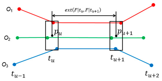
Figure 1.
Illustration of the spatial extent of a flock over two consecutive timestamps.
Definition 5
(Improved moving flock). Given a set of n trajectories, an (r, m, k, d)-moving flock FM during a time interval where consists of at least m objects such that for each discrete timestamp there exists a disk of radius r containing all m objects and every spatial extent between two consecutive timestamps . Assuming that the m objects are O1, O2, …, Om, respectively, then FM can be represented as .
It should be noted that Definition 5 is applied here and throughout as the definition of moving flock.
3. Taxonomy of Flock Patterns
While existing definitions and methods have enhanced the discovery of flock patterns in movement data, classifications of flock patterns remain fragmented. Hence, establishing a comprehensive taxonomy of flock patterns is essential. In this paper, we develop a taxonomy of flock patterns based on the definitions of flock and moving flock introduced in Section 2. To the best of our knowledge, this is the first attempt to systematically categorize flock patterns in this way.
The taxonomy is primarily developed using the four parameters discussed in Section 2 (i.e., r, m, k, d). Here, r identifies group members that are spatially close within a flock, and m determines the required number of group members. Together, r and m form the “number of members” factor. k represents the “time duration” factor, while d distinguishes between a stationary flock and a moving flock, making it the “displacement” factor. For the “number of members” factor, values can be the minimum, the maximum, or intermediate. Similarly, for the “time duration” factor, values can be the shortest, the longest, or intermediate. Thus, each of these two factors has three possible values. For the “displacement” factor, values have two cases: smaller than a predefined distance threshold, or not smaller than a predefined distance threshold. Based on the value cases for all three factors, 18 (i.e., 3 × 3 × 2) types of flock patterns can be derived. The classification of the 18 types of flock patterns within the developed taxonomy is shown in Table 1. Among them, nine types (types 2, 4, 6, 8, 10, 12, 14, 16, and 18) represent moving flock patterns, while the remaining nine denote stationary flock patterns. Given that our primary objective is to discover moving flock patterns, we focus on these nine types of moving flock patterns.

Table 1.
The classification of the 18 types of flock patterns derived according to the taxonomy.
Theoretically, each of the nine types of moving flock patterns has distinct significance, and different types may attract different levels of interest. However, in practice, not all types of moving flock patterns are equally interesting. In particular, those patterns where factors assume extreme values, such as the smallest/largest number of members and the shortest/longest time duration, may be of greater interest. Among the nine types in Table 1, only four types (types 2, 6, 14, and 18) fulfill these criteria. Therefore, this paper focuses specifically on these four types of moving flock patterns, which we label as types A, B, C, and D, respectively. An overview of these four types and their corresponding interpretations is provided in Table 2. Each type may indicate a distinct and valuable movement behavior in practical scenarios, with type A generally occurring most frequently, types B and C at intermediate frequencies, and type D least frequently. Due to its unique characteristics, type D may be undetectable in many instances; however, we still include it in our analysis as it can be detected under certain conditions.
Table 2.
The four different types of moving flock patterns and their interpretations.
4. Methodology
In this paper, we propose a Reeb graph-based approach for discovering moving flock patterns. Generally, the approach includes five steps: (1) generating Reeb graphs based on movement data; (2) filtering specific Reeb graphs; (3) extracting flock patterns; (4) discovering moving flock patterns, and (5) discovering the four distinct types of moving flock patterns. The framework of the methodology is shown in Figure 2. Each of these steps is described in detail below.
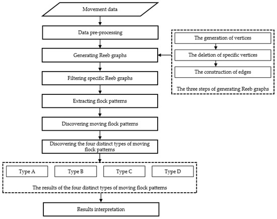
Figure 2.
The framework of the methodology.
To facilitate understanding, we use a sample dataset to demonstrate the approach. The dataset, shown in Figure 3a, illustrates the movements of seven objects. Five objects (the IDs are 1, 2, 3, 4, and 5) are tracked during a time interval consisting of five consecutive timestamps (i.e., t0, t1, t2, t3, and t4), and two objects (the IDs are 6 and 7) are tracked during a time interval consisting of two consecutive timestamps (i.e., t2 and t3). The discrete points denote the spatial locations of each object at the corresponding timestamps.
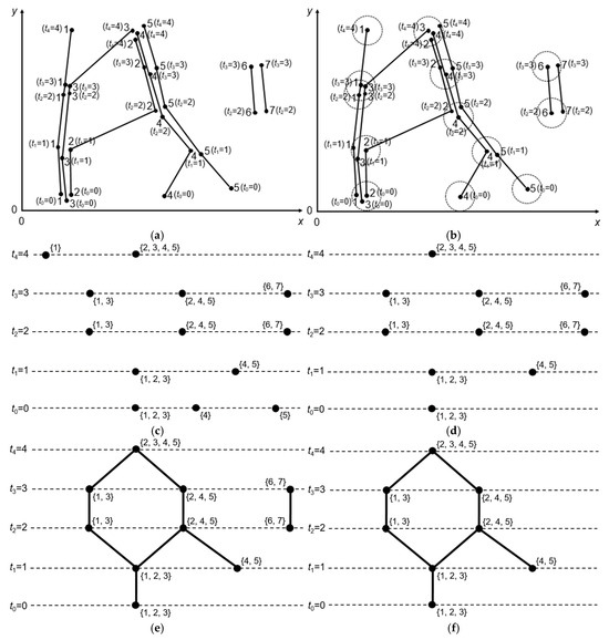
Figure 3.
Illustration of the methodology: (a) the sample dataset; (b) the groups of objects at each timestamp according to parameter r; (c) the generated vertices; (d) the remaining vertices after removing certain vertices; (e) the generated Reeb graphs, and (f) the remaining Reeb graph.
4.1. Generating Reeb Graphs Based on Movement Data
The Reeb graph, originating from topology, has been widely applied in various fields, especially in shape analysis [36,37] and visualization of scientific data [38,39]. Due to its robust capability to represent the evolution of connected components of the level sets on a two or higher dimensional scalar function, the Reeb graph has also been introduced in trajectory analysis [40,41]. Essentially, it is a structure that captures temporal changes in the spatial proximity of groups of moving objects, making it an effective tool for representing the evolution of grouping structures of moving objects over time.
In this paper, the Reeb graph is generated based on regularly sampled movement data. Similar to other types of graphs, the Reeb graph can be represented as , where and denote the sets of vertices and edges, respectively. Generally, two steps are required to construct a Reeb graph: (1) the generation of vertices, and (2) the construction of edges. To reduce computational costs, we propose generating simplified Reeb graphs rather than complete Reeb graphs. A simplified Reeb graph is derived by removing certain vertices (and their corresponding edges) from the initial complete Reeb graph. For simplicity, we refer to the simplified Reeb graph as the Reeb graph throughout the paper. In general, generating a simplified Reeb graph involves three steps: (1) the generation of vertices; (2) the deletion of specific vertices, and (3) the construction of edges.
4.1.1. The Generation of Vertices
The generation of vertices relies on the parameter r. If multiple objects have spatial locations within a circle of radius r at the same timestamp, they are considered to belong to the same vertex. It should be noted that the selection of the base object (i.e., the object whose spatial location at a given timestamp serves as the center of the corresponding circle) is important. In this approach, we propose that, for each timestamp, the base object is automatically determined as the one closest (in terms of Euclidean distance) to the centroid of all objects at that timestamp. This method enables consistent base object selection, thus can avoid variations of results caused by random selections of the base objects. The vertices of the Reeb graphs are generated according to the following four steps.
- Step 1: for each timestamp, calculate the centroid of the spatial locations of all objects;
- Step 2: find the object closest to the centroid in terms of spatial distance, and consider this object as a base object;
- Step 3: find all objects whose spatial distances to the base object are no larger than r, and group these objects with the base object in the same vertex;
- Step 4: for the remaining objects, repeat steps 1~3 until each object at every timestamp is assigned to a vertex.
Using the proposed approach, objects at each timestamp can be partitioned into one or more groups, with each group consisting of objects located within a circle of radius r. For example, if we assume that r is set to a specific value in Figure 3a, the resulting groups of objects are shown in Figure 3b. The vertices of the Reeb graphs are illustrated in Figure 3c, where each point represents a vertex, and the numbers next to each vertex indicate the IDs of the objects included in that vertex.
4.1.2. The Deletion of Specific Vertices
In certain cases, vertices may contain fewer than m objects. In these instances, such vertices must be removed. The method for deleting these vertices is described as follows.
- Step 1: for each vertex, calculate the number of objects involved in it;
- Step 2: if the number is less than m, delete the vertex;
- Step 3: repeat steps 1~2 until all vertices have been checked.
4.1.3. The Construction of Edges
When constructing edges, the following two principles are applied: (1) no two vertices at the same timestamp are connected, and (2) any two vertices at two consecutive timestamps are connected if they share at least one common object.
4.2. Filtering Specific Reeb Graphs
The filtering of specific Reeb graphs is achieved based on the parameter k. If the time duration of a Reeb graph is shorter than k, that Reeb graph must be filtered out. The method for filtering these Reeb graphs is described as follows.
- Step 1: for each Reeb graph, find its minimum timestamp and maximum timestamp , if , delete this Reeb graph;
- Step 2: repeat step 1 until all Reeb graphs have been checked.
4.3. Extracting Flock Patterns
All Reeb graphs constructed to date satisfy the flock criteria, which means that each Reeb graph meets the following conditions: (1) the objects involved in each vertex are within a circle of radius r; (2) the number of objects involved in each vertex is not less than m, and (3) the time duration of each Reeb graph is not less than k. Based on each Reeb graph, one or more flocks can be extracted. The detailed procedure for extracting flock patterns based on each Reeb graph is described below.
- Step 1: for a vertex , find all subgroups (each of which consists of at least m objects) that can be formed by the objects involved in it;
- Step 2: start with the first subgroup; if this subgroup has not been processed, proceed to the next vertex connected to . If this subgroup can also be formed in , go to the next vertex connected to . Once the subgroup can no longer be maintained, record the timestamps for its start and end, and mark this subgroup as processed;
- Step 3: for any unprocessed subgroups formed by the objects involved in , repeat step 2 until all subgroups are processed, and discard the subgroups with time durations shorter than k;
- Step 4: for the vertex , repeat similar operations as shown in steps 1~3.
Taking Figure 3f as an example, assuming m is set to 2 and k is set to 2, five flocks can be extracted: , , , and , respectively.
4.4. Discovering Moving Flock Patterns
However, among the extracted flock patterns, not all qualify as moving flock patterns. The method for discovering moving flock patterns is described below.
- Step 1: for each flock pattern , assume the corresponding time interval of is , calculate the spatial extent of between and , if , the time interval is divided into two sub time intervals, i.e., and . Repeat this process until the spatial extent of between any two consecutive timestamps is checked. Thus, is divided into multiple sub flock patterns if there exist time intervals during which the objects involved in appear stationary.
- Step 2: repeat step 1 until all flock patterns have been checked.
Based on the above method, a set of sub flock patterns can be generated for certain flock patterns if there are time intervals during which the involved objects remain stationary. However, if the duration of any generated sub flock pattern is shorter than k, it must be discarded. Finally, the remaining flock patterns are considered as moving flock patterns.
For example, in Figure 3b, the spatial extent of flock between and does not meet the requirement for a moving flock, so it is split into two sub flocks: and . Assuming m is set to 2 and k is set to 2, is not considered as a flock because the duration for which objects 1 and 3 remain close to each other is less than 2. Hence, based on the flock patterns extracted in Section 4.3, the final moving flock patterns are , , , , and .
4.5. Discovering the Four Distinct Types of Moving Flock Patterns
In this paper, we primarily focus on the four distinct types of moving flock patterns listed in Table 2. The method for discovering each of the four types of moving flock patterns is described below.
- Step 1: assume there are n moving flock patterns , for each moving flock pattern (), calculate the number of objects involved in it and the corresponding time duration. Assume that the results are and , respectively;
- Step 2: repeat step 1 until all moving flock patterns have been checked. The final results are stored in two collections N and T, respectively, where and ;
- Step 3: calculate the minimum and maximum values of N and T, denoted as min_N, max_N, min_T and max_T, respectively;
- Step 4: each of the four distinct types of moving flock patterns is discovered based on the following criteria.
- Type A: determine the moving flock patterns whose time duration is equal to min_T and the number of objects involved is equal to min_N in ;
- Type B: determine the moving flock patterns whose time duration is equal to max_T and the number of objects involved is equal to min_N in ;
- Type C: determine the moving flock patterns whose time duration is equal to min_T and the number of objects involved is equal to max_N in ;
- Type D: determine the moving flock patterns whose time duration is equal to max_T and the number of objects involved is equal to max_N in .
Based on this method, all four types of moving flock patterns can be extracted. Take the sample dataset in Figure 3 for instance, the four types of moving flock patterns are listed in Table 3.
Table 3.
The four distinct types of moving flock patterns being discovered in the sample dataset.
5. Case Study
5.1. Dataset
The movement data used in this study originated from a real and complete football match between Club Brugge KV and Standard de Liège that took place on 2 March 2014. For simplicity, we refer to them as Club Brugge and Standard Liège throughout this paper. The dataset includes both spatiotemporal and semantic information. The spatiotemporal information is recorded in the format (id, x, y, t), where id identifies a particular player, x and y denote the x and y coordinates of the player’s position, and t represents the corresponding timestamp. The semantic information mainly includes the basic information of both teams (e.g., players’ names, players’ IDs, and played positions) and the events that occurred during the match (e.g., event name, time of occurrence, and IDs of the actors). The spatiotemporal information can be used to discover moving flock patterns based on the approach proposed in this paper, and the semantic information can be used to validate the discovered moving flock patterns if necessary.
As football is considered a highly interactive sport in which players need to interact frequently with their teammates, various types of interaction patterns may be involved. Among them, moving flock patterns are of particularly interest in this study, as discovering and exploring these patterns can provide valuable insights into a team’s playing style, which could inform tactical assessments. This paper emphasizes methodology, so we focused only on the movement data of Club Brugge’s outfield players (excluding the goalkeeper) during the first five minutes. This early match period is often crucial, as coaches typically provide tactical instructions before the match and aim to evaluate them in these initial moments. In the original dataset, the locations of all players were tracked with a temporal resolution of 0.1 s. To reduce computational complexity, we down-sampled this to 1 s. After processing, 3010 discrete points and 10 trajectories were generated, and they are visualized in Figure 4. For privacy reasons, the ten players are labeled as player 1, player 2, player 3, …, and player 10.
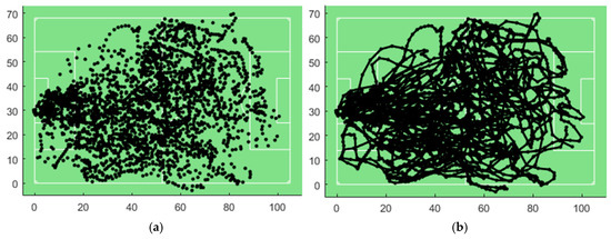
Figure 4.
Visualization of the movement data: (a) the discrete points, and (b) the corresponding trajectories.
5.2. Results and Analysis
As mentioned above, four parameters are involved in the proposed approach, which can result in different moving flock patterns depending on different parameter values. To examine how these parameter values affect the number of detected moving flock patterns, we analyzed the relationship between varying a single parameter and the resulting number of patterns, while keeping the other three parameters at default values. The initial default values of the four parameters are listed in Table 4. The initial default values were chosen for two main reasons: (1) each parameter’s default value was balanced (neither too large nor too small) based on our preliminary experiments, and (2) a relatively large number of moving flock patterns could be discovered, based on which substantial and useful information was provided. The relationships between each parameter value and the number of moving flock patterns discovered are shown in Figure 5.
Table 4.
The default values of the four parameters.
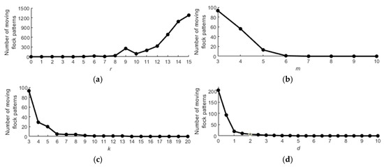
Figure 5.
The relationships between the values of the parameters and the number of moving flock patterns detected: (a) r; (b) m; (c) k, and (d) d.
Figure 5 shows that for parameter r, the number of moving flock patterns generally rises as r increases, with an outlier at r = 9. According to our improved definition of moving flock, a flock must be divided into smaller moving flocks if the spatial extent between two specific consecutive timestamps is less than d. This leads to an increase of detected moving flock patterns, making the sharp rise when r = 9 understandable. Based on our improved definition, many finer moving flocks could be detected instead of a single large moving flock, so the number of moving flock patterns does not necessarily increase continuously with r. This is different from the previous results of Wachowicz et al. [32], who observed a direct correlation between increasing r and the number of patterns. This distinction is a significant finding in our research. Additionally, when r equals to 9, the number of moving flock patterns is suitable (neither too large nor too small), so 9 seems to be a favorable value for r. For the parameters m, k and d, the number of moving flock patterns decreases as these values increase. However, when values exceed certain thresholds, no moving flock patterns are detected. Thus, the initial default values for m, k and d listed in Table 4 appear to be well-chosen.
The relationships between the parameter values and the number of detected moving flock patterns (types A~D) are shown in Figure 6. From Figure 6, it can be seen that the number of type A is obviously large when each parameter meets certain requirements (e.g., r ≥ 9/m ≤ 4/k ≤ 5/d ≤ 1). In contrast, the number of type D is the smallest among the four types for each parameter. For types B and C, the number is usually between types A and D. Therefore, we can see that type A generally always has a larger number than the other three types (when r exceeds a certain threshold or m/k/d is below certain values), and the number of type D is always quite small or even zero. This observation is intuitive since types A and D represent two extremes. Hence, Figure 6 shows that the results of the four types of detected moving flock patterns align well with expectations.
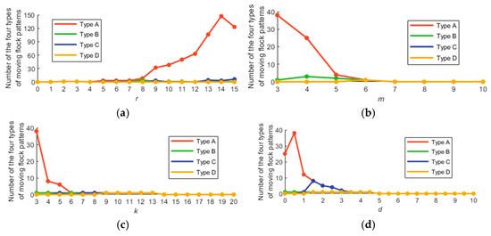
Figure 6.
The relationships between the parameter values and the number of the four different types of moving flock patterns detected: (a) r; (b) m; (c) k, and (d) d.
In addition to individual parameter values, the combination of different parameter values can also influence the number of moving flock patterns being discovered. Therefore, it is essential to find a suitable value for each parameter. To achieve this, we performed a hierarchical clustering on the four parameters, as shown in Figure 5. The reason is that hierarchical clustering helps reveal similarities and dissimilarities progressively, enabling us to suggest optimal parameter values that can be adjusted to meet specific requirements. The resulting hierarchical clustering is shown in Figure 7, in which a higher link shows that the corresponding elements are more different from each other. Thus, the optimal parameter values can be determined based on the desired degree of similarity. Since football is typically considered as a complex dynamic interaction among players, the optimal values require further refinement. For parameter r, values 14 and 15 are the most dissimilar but are not considered optimal, as they produce an excessive number of moving flock patterns, which does not yield satisfactory results, as shown in Figure 4a. Therefore, values with lower dissimilarity level (i.e., 9 or 12) appear more suitable, and based on the outlier in Figure 4a, 9 was chosen as the optimal value for r. Regarding parameter m, a setting of 3 resulted in many moving flocks involving fewer players. However, since complex tactics generally involve larger groups of players, such flocks are more useful for performance evaluation. For this reason, we consider the optimal value for m to be 4 (i.e., the value with the second highest dissimilarity). For parameter k, since we aimed to detect moving flock patterns involving more players for performance assessment, the duration of the moving flocks was less critical for us. Therefore, 3 was an appropriate value for k. When the parameter d is 0, it means that the flocks are stationary. As we are interested in moving flocks, 0.5 seemed to be an optimal value for d. Therefore, according to Figure 6, the optimal values for the four parameters are: r = 9, m = 4, k = 3 and d = 0.5. Note that the optimal values may be different for different scenarios, so one has to choose the appropriate parameter values depending on the specific objectives.
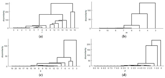
Figure 7.
Hierarchical clustering of the four parameters: (a) r, (b) m, (c) k, and (d) d.
We therefore tested the proposed approach with the optimal parameter combination: r = 9, m = 4, k = 3 and d = 0.5. Finally, 72 moving flock patterns were discovered. However, since not all parameters were of particular interest, we extracted the four distinct types of moving flock patterns, the total number of which was 21. The exact number of each type is listed in Table 5.
Table 5.
Number of the four distinct types of moving flock patterns detected under the parameter combination r = 9, m = 4, k = 3 and d = 0.5.
From Table 5, it can be seen that the number of type A was comparatively large. This shows that many moving flock patterns involve the fewest players over the shortest time duration. In contrast, patterns with the minimum number of players and the longest time duration (type B) or the maximum number of players and the shortest time duration (type C) were less frequent. Furthermore, there was no pattern with both the maximum number of players and the longest time duration (type D). To examine the detected moving flocks more closely, we provides the detailed information (i.e., the players involved and the corresponding time intervals) for each type of moving flock pattern in Table 6. For brevity, we arbitrarily selected three moving flocks of type A for illustration. Each moving flock in Table 6 indicates that the players were within a certain circle at the same timestamp and continued to move during the corresponding time intervals. For example, the moving flock {1, 5, 8, 10}|[240, 243] indicates that players 1, 5, 8 and 10 moved during 240 s~243 s, and at each timestamp (i.e., 240 s, 241 s, 242 s and 243 s) their spatial positions were within a circle of radius 9 m. Based on the discovered moving flocks, sports professionals can explore the dynamic interactions among players for effective performance analysis. The moving flock patterns listed in Table 6 are visualised and depicted in Figure 8. To aid interested readers in interpreting these patterns, we show more detailed information in Figure 9, including the IDs of the players and their exact trajectories. For clarity, we use the red dots in relatively large size, rather than traditional arrows, to indicate the endpoints of the corresponding trajectories.
Table 6.
Detailed information on the four different types of illustrated moving flock patterns under the parameter combination: r = 9, m = 4, k = 3, and d = 0.5.
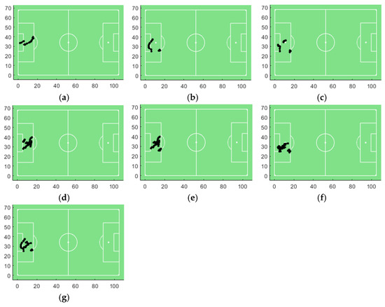
Figure 8.
Visualization of the illustrated moving flock patterns under the parameter combination r = 9, m = 4, k = 3, and d = 0.5 (listed in Table 6): (a) {1, 5, 8, 10}|[240, 243]; (b) {1, 3, 4, 5}|[249, 252]; (c) {1, 3, 4, 8}|[253, 256]; (d) {5, 8, 9, 10}|[244, 252]; (e) {4, 8, 9, 10}|[244, 252]; (f) {3, 4, 9, 10}|[249, 257], and (g) {1, 3, 4, 5, 8, 9, 10}|[249, 252].
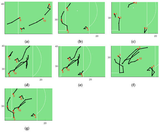
Figure 9.
Detailed information of the moving flock patterns shown in Figure 7: (a) {1, 5, 8, 10}|[240, 243]; (b) {1, 3, 4, 5}|[249, 252]; (c) {1, 3, 4, 8}|[253, 256]; (d) {5, 8, 9, 10}|[244, 252]; (e) {4, 8, 9, 10}|[244, 252]; (f) {3, 4, 9, 10}|[249, 257], and (g) {1, 3, 4, 5, 8, 9, 10}|[249, 252].
Figure 8 indicates that the spatial variations of the four types of moving flock patterns listed in Table 6 are generally minimal. According to the semantic information in the dataset, it appears that the match was temporarily interrupted during these time intervals (e.g., by a “clearance” event), which likely caused the reduced spatial variation, as the players were not moving at high speed. An important reason for this could be that 0.5 is not a very large value for the parameter d. Nevertheless, we can see from Figure 9 that the players in the same group can indeed form a moving flock, as they met the criteria of a moving flock. This demonstrates that the proposed approach effectively detects moving flock patterns and accurately distinguishes the four different types of moving flock patterns.
To further validate the proposed approach, we also tested an alternative parameter combination: r = 15, m = 4, k = 3, and d = 2. The reason is that with this parameter combination, more moving flock patterns should be detected, and the spatial variations of the detected moving flock patterns should be larger. The results show that a total of 94 moving flock patterns were found with this parameter combination. The number for each of the four distinct types of moving flock patterns, along with detailed information of the selected examples (the first three moving flocks of each type if there are more than three) are listed in Table 7 and Table 8, respectively. The moving flock patterns listed in Table 8 are visualized in Figure 10, and the moving flock patterns in Figure 10 are shown with more detailed information (i.e., the IDs of the players and the exact trajectories, using the same visualization strategy as in Figure 8) in Figure 11.
Table 7.
Number of the four different types of moving flock patterns detected under the parameter combination: r = 15, m = 4, k = 3, and d = 2.
Table 8.
Detailed information on the four different types of illustrated moving flock patterns under the parameter combination: r = 15, m = 4, k = 3, and d = 2.
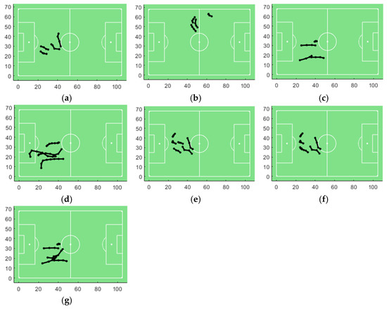
Figure 10.
Visualization of the illustrated moving flock patterns under the parameter combination r = 15, m = 4, k = 3, and d = 2 (listed in Table 8): (a) {1, 4, 5, 7}|[14, 17]; (b) {1, 4, 9, 10}|[131, 134]; (c) {2, 5, 6, 9}|[174, 177]; (d) {1, 2, 6, 7}|[175, 182]; (e) {1, 2, 4, 7, 8, 9}|[15, 18]; (f) {1, 4, 7, 8, 9, 10}|[15, 18], and (g) {1, 2, 5, 6, 7, 9}|[174, 177].
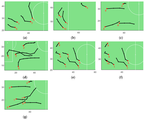
Figure 11.
Detailed information of the moving flock patterns shown in Figure 9: (a) {1, 4, 5, 7}|[14, 17]; (b) {1, 4, 9, 10}|[131, 134]; (c) {2, 5, 6, 9}|[174, 177]; (d) {1, 2, 6, 7}|[175, 182]; (e) {1, 2, 4, 7, 8, 9}|[15, 18]; (f) {1, 4, 7, 8, 9, 10}|[15, 18], and (g) {1, 2, 5, 6, 7, 9}|[174, 177].
Figure 10 reveals that the overall spatial variations of the seven moving flock patterns were larger than those shown in Figure 8. Upon examining the semantic information, we found that the players were either passing, receiving, or running with the ball during the time intervals listed in Table 8, contributing to the increased spatial variation. Additionally, we can see that the trajectories of the players in the same moving flock shown in Figure 11 were generally more regular than those shown in Figure 9, suggesting that the players in these flocks may have been employing a coordinated tactic.
Figure 7, Figure 8, Figure 9 and Figure 10 demonstrate that the proposed approach effectively detects moving flock patterns, with distinct spatial variations corresponding to different event contexts. By adjusting the parameter values appropriately, it is possible to identify moving flock patterns that align with specific requirements. This flexibility allows for the selection of tailored parameter values to capture desired moving flock patterns based on varying objectives.
Moreover, the group of players involved in the same moving flock for multiple times (similar to the top-k flock patterns in [30]) appears interesting, because these players may interact strongly and frequently with each other. This information could assist coaches in refining tactical strategies. We also provide an additional feature to identify such groups of players based on the discovered moving flock patterns. For illustration purposes, the five most significant player groups that appeared in the discovered moving flock patterns under the two parameter combinations mentioned above are listed in Table 9 and Table 10, respectively. In these two tables, the first column represents the player group and the second column represents the number of appearances of the group. These insights could provide sports professionals (e.g., coaches) with valuable suggestions for tactical adjustments.
Table 9.
The five most common player groups in all detected moving flock patterns under the parameter combination: r = 9, m = 4, k = 3, and d = 0.5.
Table 10.
The five most common player groups in all detected moving flock patterns under the parameter combination: r = 15, m = 4, k = 3, and d = 2.
6. Discussion
We propose a Reeb graph-based approach for discovering moving flock patterns. The results show that the proposed approach effectively identifies desired moving flock patterns and provides valuable insights for sports professionals. Validated using real-world data from a football match, the results demonstrate the effectiveness and utility of the proposed approach in discovering and analyzing moving flock patterns. By delivering actionable tactical insights, this approach supports improved strategic planning and more informed decision-making during matches. The main contributions of this research, in comparison to existing studies, are summarized in Table 11.
Table 11.
The main contributions of this research compared to existing studies.
In this approach, the movement data are transferred into simplified Reeb graphs, which are subsequently used for further operations, enhancing the efficiency of the algorithm. However, this approach does not fully capture the overall changes (e.g., spatial configuration) of all moving objects over time, which could be a limitation since some of this information may be highly valuable. In the future, the complete Reeb graphs could be incorporated to address this limitation by providing more comprehensive insights. However, careful consideration will be required for balancing the completeness of information with algorithmic efficiency.
When generating the vertices of a Reeb graph, we adopted a strategy of first automatically determining a base object for each group and then grouping all objects within a radius r as part of that a group. Different methods for defining these circular boundaries naturally yielded varying group results, and alternative strategies could be developed to construct corresponding circles. A thorough comparison of different circle construction strategies/algorithms could help users define groups more effectively based on their needs. Moreover, the proposed approach involves four parameters and the effects of the four parameters on the results were analyzed. While we suggest a way for selecting appropriate parameter values, the selection of optimal parameter values is still an open question.
The proposed Reeb graph-based approach has proven effective in discovering various moving flock patterns, which provides valuable insights. However, a recurring issue is the potential overlap among the detected moving flock patterns, either in group members, time intervals or both (as can be seen in Table 6 and Table 8). This overlap may introduce a degree of redundancy, limiting the clarity of the overall evolutionary trajectory of the moving objects involved. While the detected patterns offer detailed snapshots, they fall short in capturing the broader progression of these dynamic groups. Therefore, in the future, this limitation may be addressed by merging overlapping moving flocks into a mega-moving flock. Such a solution may illuminate the complex interactions and underlying mechanisms shaping the behaviors of these moving objects.
7. Conclusions
Movement data has become widespread in a variety of fields, making it a prevalent data type, especially for research focused on discovering movement patterns. In this paper, first, an improved definition of moving flock is developed, allowing for a more refined characterization of moving flock patterns compared to previous definitions. Second, a taxonomy of flock patterns is proposed, which distinguishes 18 different types of flock patterns (including nine types of stationary flock patterns and nine types of moving flock patterns). Among them, this paper focuses on four distinct types of moving flock patterns. Third, a Reeb graph-based approach is proposed to discover the four types of moving flock patterns. In general, the proposed approach includes five steps: (1) generating Reeb graphs based on movement data; (2) filtering specific Reeb graphs; (3) extracting flock patterns; (4) discovering moving flock patterns; and (5) discovering the four distinct types of moving flock patterns. The approach was validated with real-world data from a football match, with results demonstrating its effectiveness in movement patterns. This enables sports professionals to gain valuable tactical insights, potentially improving strategic planning and decision-making during matches.
Given the importance of research on moving flock patterns and possible extensions of the proposed approach, we summarize some avenues for future research. Although the proposed approach has been validated with data from a single football match, this dataset is relatively limited in size. Future research could apply the approach to larger datasets, such as comprehensive movement data from entire matches or even multiple games. This expansion could uncover a broader array of moving flock patterns and offer more granular insights for sports professionals, aiding in strategic and tactical planning. Additionally, given the strong applicability of the proposed approach, movement data from various domains, such as urban traffic analysis, animal migration studies, or crowd dynamics, can be incorporated to explore new types of moving flock patterns. Broadening the dataset domains would not only test the robustness of the proposed approach but also provide domain-specific insights, expanding the impact and relevance of the research.
Author Contributions
Conceptualization, P.Z. and N.V.d.W.; data curation, N.V.d.W.; formal analysis, P.Z. and N.V.d.W.; funding acquisition, P.Z.; investigation, P.Z.; methodology, P.Z. and N.V.d.W.; software, P.Z.; validation, P.Z.; visualization, P.Z.; writing—original draft, P.Z.; writing—review and editing, P.Z. and N.V.d.W. All authors have read and agreed to the published version of the manuscript.
Funding
This research was supported by grants from the Introduction Program of High-Level Innovation and Entrepreneurship Talents in Jiangsu Province (Grant No. CZ032SC20025), the NUPTSF (Grant No. NY219140), and the Smart Health Big Data Analysis and Location Services Engineering Lab of Jiangsu Province (Grant No. SHEL221004).
Institutional Review Board Statement
Not applicable.
Informed Consent Statement
Not applicable.
Data Availability Statement
The data presented in this study are available on request from the corresponding author due to privacy restrictions.
Acknowledgments
The authors would like to thank the anonymous reviewers for their valuable comments and suggestions to improve the manuscript.
Conflicts of Interest
The authors declare no competing interest.
References
- Wu, X.H.; Dong, W.H.; Wu, L.; Liu, Y. Research themes of geographical information science during 1991–2020: A retrospective bibliometric analysis. Int. J. Geogr. Inf. Sci. 2023, 37, 243–275. [Google Scholar] [CrossRef]
- Oueslati, W.; Tahri, S.; Limam, H.; Akaichi, J. A systematic review on moving objects’ trajectory data and trajectory data warehouse modeling. Comput. Sci. Rev. 2023, 47, 100516. [Google Scholar] [CrossRef]
- Liu, Q.L.; Zhu, S.C.; Deng, M.; Liu, W.K.; Wu, Z.H. A spatial scan statistic to detect spatial communities of vehicle movements on urban road networks. Geogr. Anal. 2022, 54, 124–148. [Google Scholar] [CrossRef]
- Yasuda, S.; Katayama, H.; Nakanishi, W.; Iryo, T. Trajectory data-driven network representation for traffic state prediction using deep learning. Int. J. Intell. Transp. Syst. Res. 2024, 22, 136–145. [Google Scholar] [CrossRef]
- Nathan, R.; Monk, C.T.; Arlinghaus, R.; Adam, T.; Alós, J.; Assaf, M.; Baktoft, H.; Beardsworth, C.E.; Bertram, M.G.; Bijleveld, A.I.; et al. Big-data approaches lead to an increased understanding of the ecology of animal movement. Science 2022, 375, eabg1780. [Google Scholar] [CrossRef] [PubMed]
- Yang, A.N.; Wilber, M.Q.; Manlove, K.R.; Miller, R.S.; Boughton, R.; Beasley, J.; Northrup, J.; VerCauteren, K.C.; Wittemyer, G.; Pepin, K. Deriving spatially explicit direct and indirect interaction networks from animal movement data. Ecol. Evol. 2023, 13, e9774. [Google Scholar] [CrossRef]
- Qin, W.T.; Tang, J.; Lu, C.; Lao, S.Y. Trajectory prediction based on long short-term memory network and Kalman filter using hurricanes as an example. Comput. Geosci. 2021, 25, 1005–1023. [Google Scholar] [CrossRef]
- Wang, J.P.; Hu, Y.J.; Duan, L.; Michailidis, G. Analysing and visualising mobility vulnerability and recovery across Florida neighbourhoods: A case study of Hurricane Ian. Reg. Stud. Reg. Sci. 2024, 11, 384–386. [Google Scholar] [CrossRef]
- Victor, B.; Nibali, A.; He, Z.; Carey, D.L. Enhancing trajectory prediction using sparse outputs: Application to team sports. Neural Comput. Appl. 2021, 33, 11951–11962. [Google Scholar] [CrossRef]
- Zhao, Y.L.; Zhang, X.Y.; Yang, M.L.; Zhang, Q.C.; Li, J.; Lian, C.; Bi, C.B.; Wang, Z.P.; Zhang, G.L. Shooting prediction based on vision sensors and trajectory learning. Appl. Sci. 2022, 12, 10115. [Google Scholar] [CrossRef]
- Li, W.J. Analyzing the rotation trajectory in table tennis using deep learning. Soft Comput. 2023, 27, 12769–12785. [Google Scholar] [CrossRef]
- Su, R.X.; Dodge, S.; Goulias, K. A classification framework and computational methods for human interaction analysis using movement data. Trans. GIS 2022, 26, 1665–1682. [Google Scholar] [CrossRef]
- Benkert, M.; Gudmundsson, J.; Hübner, F.; Wolle, T. Reporting flock patterns. Comput. Geom. 2008, 41, 111–125. [Google Scholar] [CrossRef]
- Fort, M.; Sellarès, J.A.; Valladares, N. A parallel GPU-based approach for reporting flock patterns. Int. J. Geogr. Inf. Sci. 2014, 28, 1877–1903. [Google Scholar] [CrossRef]
- Han, W.; Wang, J.; Wang, Y.; Xu, B. Multi-UAV flocking control with a hierarchical collective behavior pattern inspired by sheep. IEEE Trans. Aerosp. Electron. Syst. 2024, 60, 2267–2276. [Google Scholar] [CrossRef]
- Yeoman, J.; Duckham, M. Decentralized detection and monitoring of convoy patterns. Int. J. Geogr. Inf. Sci. 2016, 30, 993–1011. [Google Scholar] [CrossRef]
- Liu, Y.Y.; Dai, H.; Li, J.W.; Chen, Y.; Yang, G.; Wang, J. BP-Model-based convoy mining algorithms for moving objects. Expert Syst. Appl. 2023, 213, 118860. [Google Scholar] [CrossRef]
- Amornbunchornvej, C.; Berger-Wolf, T.Y. Mining and modeling complex leadership-followership dynamics of movement data. Soc. Netw. Anal. Min. 2019, 9, 58. [Google Scholar] [CrossRef]
- Gao, J.; Gu, C.G.; Shen, C.S.; Yang, H.J. Tree structures may be the leadership structures employed by group motions exhibiting hierarchy. Phys. Rev. Res. 2024, 6, 043058. [Google Scholar] [CrossRef]
- Kalnis, P.; Mamoulis, N.; Bakiras, S. On discovering moving clusters in spatiotemporal data. In International Symposium on Spatial and Temporal Databases; Springer: Berlin/Heidelberg, Germany, 2005; pp. 364–381. [Google Scholar]
- Loglisci, C. Using interactions and dynamics for mining groups of moving objects from trajectory data. Int. J. Geogr. Inf. Sci. 2017, 32, 1436–1468. [Google Scholar] [CrossRef]
- Laube, P.; Imfeld, S. Analyzing relative motion within groups of trackable moving point objects. Lect. Notes Comput. Sci. 2002, 2478, 132–144. [Google Scholar]
- Laube, P.; van Kreveld, M.; Imfeld, S. Finding REMO—Detecting relative motion patterns in geospatial lifelines. In Proceedings of the 11th International Symposium on Spatial Data Handling, Leicester, UK, 23–25 August 2004; pp. 201–214. [Google Scholar]
- Eppstein, D.; Goodrich, M.; Sun, J. The skip quadtree: A simple dynamic data structure for multidimensional data. In Proceedings of the 21st ACM Symposium on Computational Geometry, Pisa, Italy, 6–8 June 2005; pp. 296–305. [Google Scholar]
- Gudmundsson, J.; van Kreveld, M. Computing longest duration flocks in trajectory data. In Proceedings of the 14th Annual ACM International Symposium on Advances in Geographic Information Systems, Arlington, VA, USA, 10–11 November 2006; pp. 35–42. [Google Scholar]
- Sanches, D.E.; Alvares, L.O.; Bogorny, V.; Vieira, M.R.; Kaster, D.S. A top-down algorithm with free distance parameter for mining top-k flock patterns. In Proceedings of the Annual International Conference on Geographic Information Science, Lund, Sweden, 12–15 June 2018; pp. 233–249. [Google Scholar]
- Mhatre, J.; Agrawal, H.; Sen, S. Efficient Algorithms for Flock Detection in Large Spatio-Temporal Data. In Proceedings of the Big Data Analytics (BDA 2019), Ahmedabad, India, 17–20 December 2019; pp. 307–323. [Google Scholar]
- Bouchard, K.; Lapalu, J.; Bouchard, B.; Bouzouane, A. Clustering of human activities from emerging movements A flocking based unsupervised mining approach. J. Ambient Intell. Humaniz. Comput. 2019, 10, 3505–3517. [Google Scholar] [CrossRef]
- Shein, T.T.; Puntheeranurak, S.; Imamura, M. Discovery of Loose Group Companion From Trajectory Data Streams. IEEE Access 2020, 8, 85856–85868. [Google Scholar] [CrossRef]
- Tritsarolis, A.; Theodoropoulos, G.S.; Theodoridis, Y. Online discovery of co-movement patterns in mobility data. Int. J. Geogr. Inf. Sci. 2021, 35, 819–845. [Google Scholar] [CrossRef]
- Ong, R.U. From Pattern Discovery to Pattern Interpretation of Semantically-Enriched Trajectory Data. Doctoral Dissertation, University of Pisa, Pisa, Italy, 2011. [Google Scholar]
- Wachowicz, M.; Ong, R.; Renso, C.; Nanni, M. Finding moving flock patterns among pedestrians through collective coherence. Int. J. Geogr. Inf. Sci. 2011, 25, 1849–1864. [Google Scholar] [CrossRef]
- Turdukulov, U.; Calderon Romero, A.O.; Huisman, O.; Retsios, V. Visual mining of moving flock patterns in large spatio-temporal data sets using a frequent pattern approach. Int. J. Geogr. Inf. Sci. 2014, 28, 2013–2029. [Google Scholar] [CrossRef][Green Version]
- Cao, Y.; Zhu, J.; Gao, F. An algorithm for mining moving flock patterns from pedestrian trajectories. Lect. Notes Comput. Sci. 2016, 9865, 310–321. [Google Scholar]
- Zhang, T.; He, W.; Huang, J.; He, Z.; Li, J. Interactive visual analytics of moving passenger flocks using massive smart card data. Cartogr. Geogr. Inf. Sci. 2022, 49, 354–369. [Google Scholar] [CrossRef]
- Biasotti, S.; Giorgi, D.; Spagnuolo, M.; Falcidieno, B. Reeb graphs for shape analysis and applications. Theor. Comput. Sci. 2008, 392, 5–22. [Google Scholar] [CrossRef]
- Chen, F.; Obermaier, H.; Hagen, H.; Hamann, B.; Tierny, J.; Pascucci, V. Topology analysis of time-dependent multi-fluid data using the Reeb graph. Comput. Aided Geom. Des. 2013, 30, 557–566. [Google Scholar] [CrossRef]
- Fomenko, A.; Kunii, T. Topological Methods for Visualization; Springer: Tokyo, Japan, 1997. [Google Scholar]
- Edelsbrunner, H.; Harer, J.L. Computational topology: An introduction; American Mathematical Society: Providence, RI, USA, 2010. [Google Scholar]
- Buchin, K.; Buchin, M.; van Kreveld, M.; Speckmann, B.; Staals, F. Trajectory grouping structure. In Proceedings of the Workshop on Algorithms and Data Structure, London, ON, Canada, 12–14 August 2013; pp. 219–230. [Google Scholar]
- Xing, X.; Yuan, Y.; Huang, Z.; Peng, X.; Zhao, P.; Liu, Y. Flow trace: A novel representation of intra-urban movement dynamics. Comput. Environ. Urban Syst. 2022, 96, 101832. [Google Scholar] [CrossRef]
Disclaimer/Publisher’s Note: The statements, opinions and data contained in all publications are solely those of the individual author(s) and contributor(s) and not of MDPI and/or the editor(s). MDPI and/or the editor(s) disclaim responsibility for any injury to people or property resulting from any ideas, methods, instructions or products referred to in the content. |
© 2024 by the authors. Licensee MDPI, Basel, Switzerland. This article is an open access article distributed under the terms and conditions of the Creative Commons Attribution (CC BY) license (https://creativecommons.org/licenses/by/4.0/).