Abstract
The lower limbs play an important role in daily human activities. Therefore, a 3D tibial model is constructed, and finite element analysis is performed to investigate the biomechanical characteristics and injury tolerance of lower limb flexion movement. The maximum equivalent stress at 30° flexion was 19.1 MPa and 31.2 MPa in the normal and dynamic eversion positions, respectively, of the knee joint, 1.4 MPa and 1.1 MPa in the medial tibial plateau, and 1.8 MPa and 1.2 MPa in the lateral tibial plateau. The peak contact force was generally approximately 4000 N when different positions of the tibia were impacted. The maximum contact force of the frontal impact was larger than that of the external impact at 4109 N and 3927 N, respectively. The dynamic knee valgus posture and lateral impacts are more likely to cause tibial injury. The findings of this study provide information for the prevention of sports injuries and rehabilitation treatment.
1. Introduction
Biomechanics is a branch of mechanics that combines the basic theories of mechanics with medicine, physiology, and other fields to conduct in-depth research on mechanical problems involved in living organisms. It greatly enriches the connotation of mechanics in terms of multiple environments and applicable objects and therefore injects new vitality into the science of mechanics. It has important theoretical and practical value in human protection, medical rehabilitation, automotive ergonomics, and other fields. Biomechanics mainly includes sports biomechanics, skeletal biomechanics, and fluid biomechanics. Due to the complexity and irregular shape of bone materials, it is difficult to obtain precise and accurate bone models using traditional modeling methods. Therefore, previous biomechanical studies have mostly utilized simplified models or cadaver experiments. They facilitate a certain degree of comprehension regarding the biomechanical characteristics of bones. However, both techniques are not without limitations. For the simplified model method, certain geometric features of bones are often ignored for the sake of convenience in calculation, or bones are treated as isotropic homogeneous materials, which will seriously affect the accuracy of the calculation results [1,2]. Firstly, the experimental materials are scarce and difficult to obtain, which makes it challenging to conduct sufficient research. Secondly, there are certain ethical constraints that limit the potential for conducting research on this topic. Therefore, the results may be limited by factors that make it difficult to obtain material values similar to those of live human bodies. Therefore, establishing a model that conforms to the geometric characteristics of human bones and has reasonable material allocation is crucial for obtaining the accurate biomechanical properties of bones.
Some abnormal movement postures of the human body can have a weak but sustained impact on human bones, which can evolve into more serious injuries over time. Due to the fact that the tibia is the main load-bearing bone in the human body, the vast majority of sports require the participation of the tibia, and the damage caused by sports to the tibia is much higher than other bones in the human body [3,4]. Buckling exercise is the most common exercise in people’s daily life and physical exercise. The so-called flexion movement refers to the joint moving around the coronal axis, causing the two bones of the relevant joint to approach each other. Therefore, studying the biomechanical characteristics of the tibia during flexion exercise and abnormal posture exercise has important theoretical and practical value for preventing sports injuries, assisting rehabilitation treatment, etc.
Impact load is the most common type of load that can cause tibial fracture injury, and the damage caused by impact load is generally more severe. However, currently, the main method for studying the biomechanical properties of the tibia under impact load in different countries is to conduct relevant experiments on the tibia of cadavers. These experiments are predominantly confined to mid-tibial impact experiments. The tolerance limit of the tibia under other impact conditions has not been sufficiently studied. Therefore, a comprehensive analysis of the impact tolerance limit of the tibia can help understand the load-bearing capacity of the lower limbs and prevent injuries. Furthermore, it can provide a foundation for the development of human rehabilitation treatments and related care.
Hu Y et al. used 3D CT simulation technology to identify different injury modes of tibial plateau fractures in flexion and analyzed the correlation between each injury mode and accompanying injuries. The research results showed that the incidence of lateral quadrant collapse fractures after type IIB fractures was significantly higher than that of type IIC fractures (p < 0.001). The incidence of posterior lateral quadrant fractures, anterior lateral quadrant fractures, and proximal fibular fractures in type IIC fractures was significantly higher than that in type IIB fractures (p < 0.001). There was a significant difference in the number of accompanying injuries between type IIB and type IIC fractures (p < 0.001) [5]. Liu et al. diagnosed anterior cruciate ligament (ACL) avulsion using data from computed tomography and magnetic resonance imaging and analyzed the 3D quantitative measurement results of tibial plateau fractures. The research results showed that there were more ACL tear and displacement during knee flexion (p < 0.05). The incidence of ACL tear in the flexion outward rotation injury mode was higher than that in other injury modes of the same level (p < 0.05). There was no significant difference in the occurrence of ACL avulsion fractures due to tibial rotation [6]. Quevedo Gonzalez F J et al. used robotic cadaver simulation to determine ankle joint kinematics to evaluate the interaction between implants and bones in total ankle arthroplasty using a finite element model (FEM). The most critical condition for the interaction between implants and bones depended on the specimen and fixation design [7]. Imhoff et al. used 3D motion tracking to capture anterior tibial translation and medial tibial rotation, analyzing the effects of ACL loss and ACL reconstruction on kinematics and ACL transplantation force during high tibial osteotomy. The combined correction of the varus and slope resulted in a corresponding decrease in tibial anterior translation in cadaveric knee joints due to ACL deficiency and reconstruction [8].
In summary, the current biomechanical methods for analyzing bones include using CT data to construct 3D models, simulating robot corpses, and 3D motion tracking. The construction of 3D models using CT data is common. However, this method may result in the loss of detailed bone information, potentially leading to an overall reduction in the accuracy of the resulting analysis [9]. Additionally, the commonly used material assignment methods are unsuitable for assigning values to bone materials due to their complex characteristics. Given this, the study is based on CT data of the lower limbs of the human body, using 3D visualization technology and a gradient grayscale assignment method to establish a FEM of the axial functional gradient of the human tibia. The FEA method is used to analyze the biomechanical characteristics of the tibia during flexion movements in different postures, as well as the tibial injury tolerance limit under different impact conditions and physiological characteristics. To accurately simulate the characteristics of the tibia, this method uses one-way linear interpolation to process CT images, increase the number of tomographic images, and reconstruct the surface of the 3D model to improve modeling quality. In addition, this study innovatively proposes a gradient grayscale assignment method, which divides the tibia into five regions, including the transition zone for material assignment, and obtains a FEM of the tibial axial functional gradient. The established tibial model was validated using statistical data on human tibial size and Yamada experimental data.
This paper is divided into five chapters. Section 2 describes the method of constructing 3D models of human tibias via FEM to increase the models’ quality. Section 3 provides an analysis of the biomechanical characteristics of lower limb flexion movement (LLFM) and the injury tolerance of the human tibia. Section 4 presents the experimental results, which includes the biomechanical properties and injury tolerance analysis of the lower limbs. Section 5 is the conclusion, which outlines the reasons for the in-depth exploration of the biomechanical properties of the lower limbs, discusses the factors that affect their injury tolerance, and summarizes the research in this article.
2. Methods and Materials
A 3D model was constructed, and the FEM of the human tibia was conducted to analyze the biomechanics and injury tolerance of LLFM.
2.1. Construction of 3D Model of Human Tibia
A 29-year-old male volunteer weighing 65 kg and standing 175 cm tall was selected for this study to construct a 3D model of the human tibia, as his tibia was considered representative of those in the population. CT scans were performed on the lower limbs of volunteers, with a slice thickness of X, an increment of 0.625 mm, a pixel size of 0.5 × 0.5 mm, and an image size of 512 × 512. There were a total of 787 images, and the image output format was DICOM 3.0. The CT image of the volunteer’s tibia is shown in Figure 1.
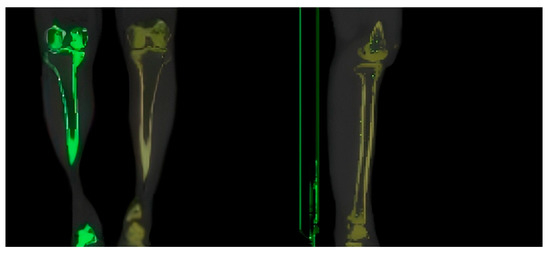
Figure 1.
CT image of the tibia of a volunteer.
Interpolation processing was required when constructing a tibial model using CT images before 3D modeling to generate new tomographic images due to the slice increment of the CT scanning being larger than the pixel size. The one-way linear interpolation method was used. This method placed each 2D fault image in the same 2D coordinate system based on spatial location parameters and then arranged them in order in space to form a 3D data field. Vertical parameters were weighted and averaged using one-way linear interpolation for each adjacent fault [10,11]. The equation for calculating the grayscale value of the inserted layer is shown in Equation (1).
is the grayscale value of pixel in the new tomographic image. and are the distances between the new fault and the images of the th and th layers, respectively. and are the grayscale values of pixel in the th and th layers of the image, respectively. Although the interpolation of CT images can improve modeling accuracy, the new tomographic image must be sharpened due to the large clarity differences between the new and original images. The Laplace operator is selected as the sharpening method, which is calculated as shown in Equation (2).
In Equation (2), is the Laplace operator, is a 2D function, and is the Cartesian coordinate. Equation (3) is obtained using a template to represent.
In Equation (3), represents the grayscale variation in the orthogonal direction. The grayscale changes in the diagonal direction are introduced because the above equation only considers the grayscale value changes in the orthogonal direction, as shown in Equation (4).
In Equation (4), and are the grayscale changes in the diagonal direction. The sharpened image is overlaid with the original CT image to obtain the final image, as shown in Equation (5).
In Equation (5), is the final image. is the original image. The image can be visualized after the CT image processing is completed. The selected visualization processing software is MIMICS 21.0. First, the CT data were imported into the software, and six display orientations were set, including up, down, left, right, front, and back. The reconstructed coronal and sagittal images were obtained after processing. Second, graphic segmentation was performed to obtain the tibial images. Segmentation based on grayscale values was an appropriate choice due to wide differences in the grayscale values among the tissues in the human body. The ability to accurately and completely extract relevant organizations depended on whether the threshold segmentation range was reasonable. If the threshold segmentation range was set too large, it would result in many irrelevant tissues in the final extraction result. If the threshold segmentation range was set too small, it would result in missing tissue to be extracted, thereby causing the constructed model to lack some features. The target tissue of this study was the human tibia, and MIMICS recommended a threshold segmentation range of 226–3071. Based on this range, the selected tissues in the three views (sagittal, coronal, and horizontal) were observed layer by layer to ascertain whether any tissues were absent or superfluous. This was done to adjust the recommended threshold segmentation range. The final tibial threshold segmentation range selected in this article was 220–2474. After threshold segmentation, there were still many other bone tissues (femur, fibula, foot bones, etc.) connected to the tibia. To extract a complete and independent tibia model, it was necessary to separate the tibia from other bones. Firstly, the Multiple Slice Edit command was used to eliminate other bone pixels connected to the tibia. This operation required extra attention to detail by observing the images in the three views to determine which pixels needed to be eliminated, otherwise the generated 3D model would not conform to the anatomical structure of the tibia. Then, the Region Growing command was used to extract independent tibial masks. Due to interference factors such as noise and vibration during CT scanning, there were some abnormal cavities in the final mask obtained, so a cavity-filling operation was required. Manually filling the cavity layer by layer was tedious. The Calculate Polylines command was used to obtain the contour line of the tibial mask plate, whether the contour line was complete layer by layer was observed, and using the contour line to fill the cavity could greatly improve work efficiency [12]. However, CT scans were affected by factors such as noise, which resulted in the presence of abnormal cavities. Therefore, the generated contour lines were used to fill the cavities.
The 3D model of the human tibia was constructed using the aforementioned method, which resulted in the formation of surface defects and an overall model that was relatively complex. Therefore, the model was first converted into a point cloud model. Then, the Geomagic Studio 2015 software was used for surface reconstruction, repairing surface defects, and streamlining the model. The first step in the surface reconstruction was point cloud simplification, which involved using a unified sampling method to reduce the number of point clouds in the model with an absolute sampling spacing of 0.48 mm. Second, the simplified point cloud model needed to be converted into a polygon model before being encapsulated with a maximum of 30 triangles during encapsulation. Mesh redrawing and noise reduction treatments were required because of the presence of surface imperfections, such as holes and nails, with the packaged model. This required setting target edge length to 0.8 mm, smoothness level to 3, smoothness to 70, and deviation limit to 1 mm. The models before and after polygon repair are shown in Figure 2.
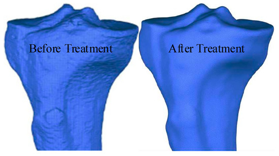
Figure 2.
Models before and after the polygon repair.
As shown in Figure 2, after polygon processing, the surface of the model was relatively smooth, without obvious defects such as holes or nails. This model was used as a basis to perform surface fitting on the tibial model. The selected surface was a NURBS surface, and the contour lines were manually drawn when performing surface fitting. Then, a surface patch (with 30 grids) was constructed based on the contour lines. Adaptive fitting considering the irregular shape of the surface patches was required to ensure the accuracy of the model. When fitting, the control point should not exceed 18 and the surface tension should be 0.3. Compared to models obtained through specialized software, the tibial 3D model obtained through the above method had good dimensional and structural universality. The axial functional gradient model could effectively avoid boundary abnormal stresses caused by discontinuous material properties, allowing the material properties of the model to continuously and smoothly change. Thus, finite element simulation results that were closer to the actual situation could be obtained. The hand-drawn contour lines and fitted tibial model are shown in Figure 3.
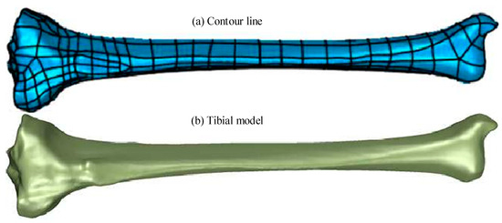
Figure 3.
Hand-drawn outline and the fitted tibia model. (a) Contour line. (b) Tibial model.
2.2. Construction of Finite Element Model of Human Tibia
After constructing the 3D model of the human tibia using the above-described methods, an FEM of the tibia based on this 3D model was built. The Three-matic 8.0 software was used to locally refine and optimize the mesh of the model to ensure its accuracy and simulation effectiveness when constructing the FEM. Compared to other software, Three-matic has the ability to highly automate the design modification, FEA/CFD pre-processing, and mold design of STL files while also enabling design modifications for complex free-form surfaces. The mesh was homogenized to ensure the accuracy and reliability of the simulation. The number of triangular meshes on the surface of the model was minimized as much as possible while retaining accuracy to reduce the size of the model. Through the above operation, high-quality surface meshes were obtained with a mesh count of 66,780. For body meshes, traditional hexahedral elements could increase simulation accuracy, but generating hexahedral elements was prone to errors due to the irregular shape of the tibia. Using the appropriate tetrahedral elements could effectively ensure simulation accuracy during biomechanical analysis [13]. Therefore, tet 10 elements were used as the body mesh of the model, with a maximum side length of 3 mm. The tet 10 elements had appropriate plasticity and creep as well as a large strain capacity. Each node had three degrees of freedom in the X, Y, and Z directions. The mesh quality distribution of the tibial model is shown in Figure 4.
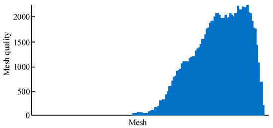
Figure 4.
Body mesh of tibial model.
In Figure 4, the quality of all grids is above the set maximum. The tibial material was assigned values after dividing the surface and body meshes of the tibial model. The common assignment methods included homogenization, binary assignment, and grayscale assignment. The homogeneous assignment method did not accurately capture the actual situation of the tibia. The binary assignment method was prone to abnormal stress mutations, and the grayscale assignment method was prone to producing non-bone materials in the model [14]. Therefore, a material assignment method based on the grayscale gradient was developed. This method divided the tibia into five regions for allocation. First, 10 layers of fault images were uniformly extracted from the small beam areas at both ends, and 20 layers of fault images were uniformly extracted in the backbone area. The MIMICS software was used to evenly set 10 detection lines on each layer of the fault image for CT value detection. Then, all data were extracted, data points within the medullary cavity were filtered and removed, and the mean method was used to obtain the average CT values of the two end-shaft and trabecular regions. Finally, the CT values were converted into material parameters and mapped to the model. This method could effectively prevent non-bone materials from appearing in the tibial model. Figure 5 shows the regional division of the tibial model.
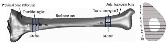
Figure 5.
Regional division of the tibial model.
As shown in Figure 5, the tibial model includes five regions: the proximal trabecular (A1), distal trabecular (A2), and diaphyseal (A3) areas and a transition zone between the proximal trabecular and diaphyseal areas (A4 and A5, respectively). The boundaries of A1 and A2 are 68 mm and 282 mm, respectively. Furthermore, the distribution of CT values must be ascertained when assigning values to tibial materials. Based on the CT value detection results, data points in the medullary cavity can be proposed to obtain the average CT values of the trabecular and diaphyseal regions at both ends. This allows for the subsequent calculation of the apparent density and Young’s modulus (YoM) of each region. This expression is shown in Equation (6).
is the apparent density, is the grayscale value, and is the YoM. Due to the varying degrees of calcification in different tibial regions, materials in the transition zone are used as functional grading materials to accurately simulate the mechanical properties of the tibia. The volume fraction of each region of the tibia is given in Equation (7).
In Equation (7), is the volume grouping of the backbone region. is the height of a certain position in the transition zone. is the length of the transition zone. is a constant that defines a change in the material composition, having a value of 0.5. is the volume fraction of A1. The YoM for the transition zone is calculated as shown in Equation (8).
represents the YoM of the transition zone. and are the style moduli of A3 and A1, respectively. Poisson’s ratio (PoR) in the transition zone is calculated using Equation (9).
In Equation (9), , , and are the PoR of the transition zone, A1, and A3, respectively. Table 1 shows the material parameters for each region.

Table 1.
Material parameters for each region of the model.
The FEM model of human lower limbs based on the above tibial model is shown in Figure 6.
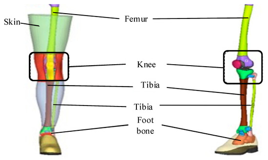
Figure 6.
A FEM model of human lower limbs.
As shown in Figure 6, during the modeling process, the lower limb surface skin was used as the outer boundary, and the lower limb femur surface was used as the inner boundary. High-quality hexahedral elements were also selected to mesh the lower limb muscle model, and a 2.5 mm-thick shell element was generated on the surface of the muscle mesh model using the faces function as the skin. The muscles and bones in the model were connected using a common node method, and the skin and muscles were also connected using a common node method. The final finite element models of the thigh and calf muscles were obtained. The focus of model development is on the long bones and knee joints of the lower limbs. By importing the established finite element models of various tissue structures of the lower limbs into finite element pre-processing software for assembly and connection adjustment, a standard 50 percentile Chinese adult male standing posture lower limb biomechanical finite element model with complete structure can be obtained.
3. Results
The biomechanical characteristics of the tibia during flexion motion were analyzed, and the damage tolerance of the human tibia under impact loading was explored.
3.1. Biomechanical Analysis of Tibia Under Flexion Movement
The FEA was conducted to investigate the biomechanical characteristics of tibial flexion in normal and dynamic knee valgus poses (DKVPs). The Workbench was used to simulate the flexion movement under normal and dynamic genu valgus positions and analyze the stress distribution of the tibia. The finite element analysis method is as follows: Due to the volunteer’s weight of 65 kg, vertical loads of 980 N, 1360 N, 1820 N, and 2360 N are applied to the meniscus area of the tibial plateau to simulate LLFM at 30°, 60°, 90°, and 120°. In normal posture, the inner and outer meniscus each bear 50% of the external force. For dynamic knee valgus posture, the lateral side of the tibial plateau bears 60% of the external load, while the medial side bears 40% of the external load. A rotational torque eM of 4 N · m is applied to the proximal end of the tibia to simulate rotational motion during tibial flexion. A horizontal external load F of 50 N is applied on the left side of the proximal tibia to simulate the inward movement of the tibia under femoral traction during dynamic knee flexion. The 25 mm-long area of the distal tibia is set as a fixed constraint. The equivalent stress curves of the flexion motion in the different poses are shown in Figure 7.
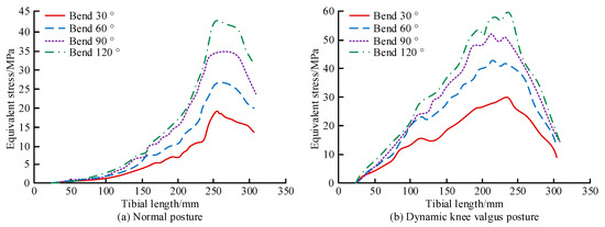
Figure 7.
Equivalent stress curves for flexion from 30° to 120° in different postures. (a) Normal posture. (b) Dynamic knee valgus posture.
Figure 7a shows that under normal posture, as the tibia lengthened, the equivalent force first increased and then decreased, reaching a maximum at 250 mm. The curve before the peak was approximately a quadratic curve. In addition, the growth rate of the equivalent stress substantially accelerated as the bending angle increased. For the four different flexion angles, the stress concentration with the normal posture mainly occurred in the anterior part of the middle and lower tibia. The peak stress roughly occurred at the junction of the middle and lower third of the tibia. Figure 7b shows that under the DKVPs, the equivalent force also first increased and then decreased, reaching a maximum at 250 mm, as the length of the tibia increased. Unlike for normal posture, the curve before the peak is close to linear. The growth rate of the equivalent force also considerably accelerated as the bending angle increased. The stress concentration in the DKVP group mainly occurred on the inner side of the middle tibia, roughly distributed along the inner edge, gradually decreasing from the middle of the tibia to both ends. The reason for this is the imbalance in the torque between the internal and external extensor muscles of the hip, which causes abnormal lateral force on the tibia. The maximum equivalent stress (MES) of the tibia and its plateau in the different poses is shown in Figure 8.
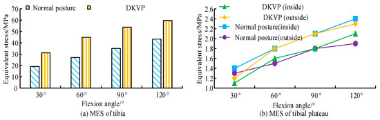
Figure 8.
MES of tibia and its plateau in different postures flexed from 30° to 120°. (a) MES of tibia. (b) MES of tibial plateau.
As shown in Figure 8a, the MES in the DKVPs was larger than that in the normal pose under the same flexion angle. For 30° and 90° flexion, the MES in the normal posture and DKVPs were 19.1 MPa/35.0 MPa and 31.2 MPa/53.8 MPa, respectively. During bending from 30° and 90° to 120°, the MES increased 29%, 22.69%, and 19.23%, respectively. Figure 8b shows that the equivalent stress of the medial tibial plateau (MTP) in the normal posture was higher than that on the lateral side, whereas the equivalent stress in the DKVPs was less than that on the lateral side. For 30° flexion, the equivalent stresses of the medial and lateral tibial plateaus in normal posture were 1.4 MPa and 1.8 MPa, respectively. Those of the DKVPs were 1.1 MPa and 1.2 MPa, respectively. The MES in the DKVPs was higher by 38.8%, 39.65%, 34.95%, and 27.52% compared with that in the normal posture group at the four different flexion angles. Dynamic knee flexion was more likely to cause substantial tibial damage due to the middle tibia having a smaller cross-sectional area than the mid-lower tibia.
3.2. Analysis of Injury Tolerance of Human Tibia
The damage to a human tibia under impact load was analyzed to investigate the damage tolerance of the human tibia. The software used for the analysis was the Workbench. The tibia showed both viscoelastic and nonlinear material characteristics during injury analysis. Therefore, the tibia was considered as an elastic–plastic material to accurately simulate the response characteristics of the tibia to impact loads. A cylindrical impact block was used, with a bottom radius of 12.5 mm, a height of 30 mm, and a mass of 6.25 kg. Steel 1006 material was used in the simulation. The impact positions were 75 mm, 175 mm, and 260 mm; the impact directions were frontal and lateral. Frictional contact was considered between the impact block and the tibia, with a friction coefficient of 0.6 and an impact velocity of 1 m/s. During the experiment, the A2 of the tibia was set as a fixed constraint, and a uniformly distributed load of 280 N was applied along the axis at the meniscus platform. The cloud map of the isoeffect force of the tibia under frontal impact is shown in Figure 9.
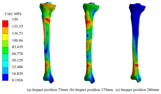
Figure 9.
Equivalent force cloud map of tibia for different impact positions. (a) Impact position 75 mm. (b) Impact position 175 mm. (c) Impact position 260 mm.
Figure 9 shows that under proximal impact, the strain at the elements near the impact point reaches failure, so the tibia begins to fracture. Stress concentrated at the distal end of the tibia due to the constraining effect of the ankle joint, but the failure strain was not reached, and no fracture occurred. Under mid-end impact, the tibia began to fracture and fail. Stress concentrated at both ends of the tibia due to the constraints of the distal ankle joint and proximal knee joint. Under distal impact, the units near the impact point reached failure strain, and the tibia began to fracture. After the tibia was impacted, the stress concentration at the impact point was larger due to the direct impact force, reaching the failure strain first, indicating that the impact point is more likely to result in fracture. The position of the distal tibial trabecular bone was subjected to a relatively high equivalent stress level when impacted due to its fixation by the ankle joint. Fractures might also occur at this location if the impact load was large enough. Figure 10 shows the contact force response and cross-sectional moment (CSM) for different impact positions.
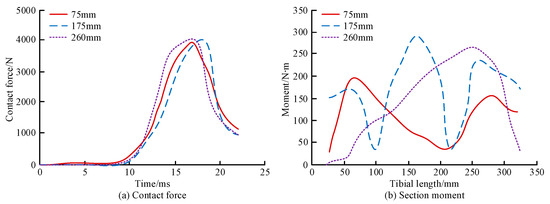
Figure 10.
Contact force response and CSM for different impact positions. (a) Contact force. (b) Section moment.
As shown Figure 10a, the contact force first increased and then decreased over time after impacts at different positions of the tibia, reaching a peak between 15 and 20 ms. The maximum contact forces of q were 3927 N, 4000 N, and 4083 N when the tibia q was impacted at 75 mm, 175 mm, and 260 mm, respectively. The maximum contact force values at three different impact positions were similar. However, the maximum contact force appeared later during mid-section impact than in the other two groups. As shown in Figure 10b, when the tibia impacts 75 mm and 175 mm, the CSM fluctuated along the length of the tibia, with peak moments of 192 N∙m and 289 N∙m, respectively. With a 260 mm impact, the tibial CSM first increased and then decreased, with a peak moment of 272 N∙m. All three impacts exhibited the largest sectional moments on the cross-section near the impact location, and the sectional bending moment of the middle impact was larger than that of the other two impacts. Figure 11 shows the contact force and CSM of the tibia for the different impact directions.
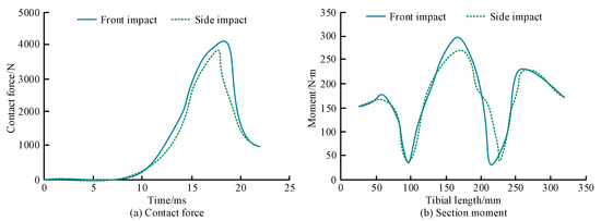
Figure 11.
Contact force and CSM of the tibia for different impact directions. (a) Contact force. (b) Section moment.
Figure 11a shows that the variation in the contact force in the tibia is consistent for the different impact directions. The maximum contact force for the frontal impacts was larger than that of the external impacts, 4109 N and 3927 N, respectively. As shown in Figure 11b, the CSM changes in the tibia for the different impact directions are also basically consistent. The ultimate torque with frontal impact was slightly higher than that with lateral impact, being 298 N∙m and 277 N∙m, respectively. The contact force of the two to contact the tibia after the impact block rises rapidly, and the bone failure falls off a cliff at the peak point. The maximum contact force of the front and rear impact is slightly larger than the left and right impact and appears slightly later. These results indicate that the tibia has a higher tolerance for frontal than lateral impact injuries. Figure 12 shows the influence of size and age on the ultimate moment of the tibia.
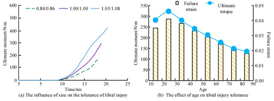
Figure 12.
The influence of size and age on the ultimate moment of the tibia. (a) The influence of size on the tolerance of tibial injury. (b) The effect of age on tibial injury tolerance. Note: x/y denotes the scaling ratio of the dimensions, where x indicates the scaling ratio of the tibial length, and y represents the scaling ratio of the lower limb width.
As shown in Figure 12a, the ultimate torque also increased as the size of the tibia increased. The ultimate moments of the tibia with scaling ratios of 0.84/0.86, 1.00/1.00, and 1.05/1.08 were 168 N∙m, 297 N∙m, and 420 N∙m, respectively. Figure 12b shows the ultimate moment and failure strain of the tibia both increase first and then decrease with age. The maximum ultimate torque and failure strain occurred at the age of 25 years, at 323 N∙m and 0.041, respectively.
4. Discussion
A 3D model of the human tibia was constructed, and FEA was conducted to investigate the biomechanical characteristics and injury tolerance of the human tibia under flexion movement. The MES of the tibia was located at 250 mm under the normal and DKVPs. In terms of positioning, under the same conditions, the MES of DKVP was greater than that of normal positioning. Taking a 30° flexion as an example, the MES for normal and DKVPs were 19.1 MPa and 31.2 MPa, respectively. DKVP was more likely to cause tibial injury than normal posture. The stress was mainly concentrated on the inner side of the muscles and bones for the DKVPs, which may be due to the imbalance in the torque between the hip abductor and abductor muscles [15,16]. The equivalent stress of the MTP in the normal posture was higher than that on the lateral side but less than that on the lateral side under DKVPs. With 30° flexion, the equivalent stresses of the medial and lateral tibial plateaus in the normal posture were 1.4 MPa and 1.8 MPa, respectively, and 1.1 MPa and 1.2 MPa under the DKVPs, respectively. This indicated that this side was more prone to shear injury due to the higher load on the lateral tibial plateau under the DKVPs [17]. This is consistent with the research findings of Wang S et al., who found that 64.1% of tibial plateau medial fractures were caused by eversion. The Wahlquist type C fractures caused by outward rotation force were significantly more than those caused by inward rotation force (p < 0.05) [18]. The study by Zhang Y et al. also demonstrated that tibial plateau fractures may be caused by outward or rotational forces, which is consistent with the results of this study [19].
In terms of tibial injury tolerance, the contact force reached a peak between 15 and 20 ms when the tibia was subjected to frontal impact. The ultimate contact force was approximately 4000 N, at which point the impact point reached the failure strain and fractures occurred. After impact, the equivalent stress in A2 remained high because the distal trabecular bone was fixed by the ankle joint and could not release stress through deformation or displacement [20]. If the impact was large enough, both the impact point and ankle might fracture. In addition, the maximum contact forces were larger for frontal than external impacts, at 4109 N and 3927 N, respectively. The ultimate torque with frontal impact was slightly larger than that of lateral impact, at 298 N∙m and 277 N∙m, respectively. The reason for the above finding might be the irregular cross-sectional shape of the tibia. Comparing the experiment with the impact test results from the cadaveric tibia specimens, the difference in the ultimate bending moment of the midsection impact was 2.4% and the maximum contact force error was 4.0%. The constructed model may be used for studying the impact injury tolerance limit of the tibia. The effects of tibial size and age on injury tolerance were also investigated. It was found that as the size of the tibia increased, its ultimate torque increased, and the tibia had the highest tolerance to injury at the age of 25 years. As age increased, bone loss gradually occurred, bone density decreased, and osteoporosis might occur [21,22].
5. Conclusions
A 3D human tibia model was constructed based on the tibia of a volunteer weighing 65 kg and standing 175 cm tall. The FEA on the model was conducted to investigate the biomechanical properties of LLFM and analyze the damage tolerance of the tibia. In the experiment, under normal and DKVPs, as the length of the tibia increased, its equivalent force first increased and then decreased, reaching a maximum at 250 mm. For the same flexion angle, the MES of the DKVPs was larger than that of the normal pose. This indicated that DKVPs were more likely to cause tibial damage. After the tibia was impacted, the equivalent stress in various regions of the tibia rapidly increased. The impact point reached failure strain the fastest, resulting in fracture, whereas the equivalent stress values on both sides of the impact point remained high but did not reach the failure strain. The stress at the A2 position on the tibia, due to its fixation by the ankle joint, was high, so A2 was also prone to injury. The biomechanical analysis of the tibia enabled the accurate prediction of the locations where the tibia was susceptible to injury during exercise. This allows for early protection and a reduction in the probability of sports injuries. Concurrently, the research method can be used to accurately ascertain the carrying capacity of the lower extremities, thereby facilitating the development of efficacious rehabilitation plans for lower limb injuries. Due to the fact that the finite element method only considers the material properties of the tibia and takes into account the damping effect of human muscles, the research results differ from the actual situation. Meanwhile, although a gradient grayscale assignment method was used to construct a tibial axial functional gradient model, the influence of porosity was ignored, and complex pores existed at both ends of the tibia. Therefore, in the future, we will comprehensively consider the interaction between muscles and tibia and establish a porous gradient model of the tibia to obtain more accurate finite element simulation results.
Author Contributions
Conceptualization, L.L. and J.-C.P.; methodology, L.L.; software, L.L. and Q.Q.; validation, L.L.; formal analysis, L.L.; investigation, H.L. (Hengjia Liu); resources, J.-C.P.; data curation, L.L.; writing—original draft preparation, L.L.; writing—review and editing, J.-C.P.; visualization, Q.Q.; supervision, L.L.; project administration, H.L. (Hongyan Liu); funding acquisition, J.-C.P. All authors have read and agreed to the published version of the manuscript.
Funding
This research received no external funding.
Informed Consent Statement
Informed consent was obtained from all subjects involved in this study.
Data Availability Statement
Data are contained within the article.
Conflicts of Interest
The authors declare no conflicts of interest.
References
- He, Y.; Shao, S.; Fekete, G.; Yang, X.; Cen, X.; Song, Y.; Sun, D.; Gu, Y. Lower Limb Muscle Forces in Table Tennis Footwork during Topspin Forehand Stroke Based on the OpenSim Musculoskeletal iModel: A Pilot Study. Mol. Cell. Biomech. 2022, 19, 221–235. [Google Scholar] [CrossRef]
- Xu, P.; Shin, I. Preparation and Performance Analysis of Thin-Film Artificial Intelligence Transistors Based on Integration of Storage and Computing. IEEE Access 2024, 12, 30593–30603. [Google Scholar] [CrossRef]
- Minematsu, A.; Nishii, Y. Effects of Whole Body Vibration on Bone Properties in Growing Rats. Int. Biomech. 2022, 9, 19–26. [Google Scholar] [CrossRef] [PubMed]
- Maghami, E.; Moore, J.P.; Josephson, T.O.; Najafi, A.R. Damage Analysis of Human Cortical Bone under Compressive and Tensile Loadings. Comput. Methods Biomech. Biomed. Eng. 2022, 25, 342–357. [Google Scholar] [CrossRef]
- Hu, Y.; Peng, A.; Wang, S.; Pan, S.; Zhang, X. Flexion tibial plateau fractures: 3-dimensional CT simulation-based subclassification by injury pattern. Orthop. Surg. 2022, 14, 543–554. [Google Scholar] [CrossRef] [PubMed]
- Liu, Z.; Wang, S.; Tian, X.; Peng, A. The relationship between the injury mechanism and the incidence of ACL avulsions in Schatzker type IV tibial plateau fractures: A 3D quantitative analysis based on mimics software. J. Knee Surg. 2023, 36, 644–651. [Google Scholar] [CrossRef]
- Quevedo Gonzalez, F.J.; Steineman, B.D.; Sturnick, D.R.; Deland, J.T.; Demetracopoulos, C.A.; Wright, T.M. Biomechanical Evaluation of Total Ankle Arthroplasty. Part II: Influence of Loading and Fixation Design on Tibial Bone–Implant Interaction. J. Orthop. Res. 2021, 39, 103–111. [Google Scholar] [CrossRef]
- Liu, H.; Zhang, H.; Lee, J.; Xu, P.; Shin, I.; Park, J. Motor Interaction Control Based on Muscle Force Model and Depth Reinforcement Strategy. Biomimetics 2024, 9, 150. [Google Scholar] [CrossRef] [PubMed]
- Salvatore, G.; Berton, A.; Orsi, A.; Egan, J.; Walley, K.C.; Johns, W.L.; Nazarian, A. Lateral Release with Tibial Tuberosity Transfer Alters Patellofemoral Biomechanics Promoting Multidirectional Patellar Instability. Arthrosc. J. Arthrosc. Relat. Surg. 2022, 38, 953–964. [Google Scholar] [CrossRef] [PubMed]
- Xiang, L.; Gu, Y.; Wang, V.F.J. Effect of Foot Pronation During Distance Running on the Lower Limb Impact Acceleration and Dynamic Stability. Acta Bioeng. Biomech. 2022, 24, 21–30. [Google Scholar] [CrossRef] [PubMed]
- Willey, M.C.; Kern, A.M.; Goetz, J.E.; Marsh, J.L.; Anderson, D.D. Biomechanical Guidance Can Improve Accuracy of Reduction for Intra-Articular Tibia Plafond Fractures and Reduce Joint Contact Stress. J. Orthop. Res. 2023, 41, 546–554. [Google Scholar] [CrossRef] [PubMed]
- Hadeed, M.M.; Prakash, H.; Yarboro, S.R.; Weiss, D.B. Intramedullary Nailing of Extra-Articular Distal Tibial Fractures: Biomechanical Evaluation of Stability Immediately After Fixation in a Synthetic Bone Model. Bone Jt. J. 2021, 103, 294–298. [Google Scholar] [CrossRef] [PubMed]
- González, F.J.Q.; Sculco, P.K.; Kahlenberg, C.A.; Mayman, D.J.; Lipman, J.D.; Wright, T.M.; Vigdorchik, J.M. Undersizing the Tibial Baseplate in Cementless Total Knee Arthroplasty Has Only a Small Impact on Bone-Implant Interaction: A Finite Element Biomechanical Study. J. Arthroplast. 2023, 38, 757–762. [Google Scholar] [CrossRef] [PubMed]
- Van den Berghe, P.; Derie, R.; Gerlo, J.; Bauwens, P.; Segers, V.; Leman, M.; De Clercq, D. Influence of Music-Based Feedback Training on Peak Tibial Acceleration During Running Outside of the Biomechanics Laboratory. Footwear Sci. 2021, 13, 39–41. [Google Scholar] [CrossRef]
- Naruse, K.; Takegami, Y.; Tokutake, K.; Shimizu, K.; Sudo, Y.; Shinohara, T.; Imagama, S. What is the Radiographic Factor Associated with Meniscus Injury in Tibial Plateau Fractures? Multicenter Retrospective (TRON) Study. Indian J. Orthop. 2023, 57, 1076–1082. [Google Scholar] [CrossRef] [PubMed]
- Shao, B.; Xing, J.; Zhao, B.; Wang, T.; Mu, W. Role of the Proximal Tibiofibular Joint on the Biomechanics of the Knee Joint: A Three-Dimensional Finite Element Analysis. Injury 2022, 53, 2446–2453. [Google Scholar] [CrossRef] [PubMed]
- Goyal, A.; Prasad, J. An in Silico Model for Woven Bone Adaptation to Heavy Loading Conditions in Murine Tibia. Biomech. Model. Mechanobiol. 2022, 21, 1425–1440. [Google Scholar] [CrossRef] [PubMed]
- Wang, S.; Peng, A.Q.; Pan, S.; Hu, Y.N.; Zhang, X.; Gao, J.G. Analysis of medial tibial plateau fracture injury patterns using quantitative 3D measurements. J. Orthop. Sci. 2021, 26, 831–843. [Google Scholar] [CrossRef] [PubMed]
- Zhang, Y.; Wang, R.; Hu, J.; Qin, X.; Chen, A.; Li, X. Magnetic resonance imaging (MRI) and computed topography (CT) analysis of Schatzker type IV tibial plateau fracture revealed possible mechanisms of injury beyond varus deforming force. Injury 2022, 53, 683–690. [Google Scholar] [CrossRef] [PubMed]
- Johnson, C.D.; Outerleys, J.; Davis, I.S. Agreement Between Sagittal Foot and Tibia Angles During Running Derived from an Open-Source Markerless Motion Capture Platform and Manual Digitization. J. Appl. Biomech. 2022, 38, 111–116. [Google Scholar] [CrossRef] [PubMed]
- Scolaro, J.A.; Wright, D.J.; Lai, W.; Fraipont, G.; Hitchens, H.; Kwak, D.; McGarry, M.; Lee, T.Q. Fixation of Extra-Articular Proximal Tibia Fractures: Biomechanical Comparison of Single and Dual Implant Constructs. J. Am. Acad. Orthop. Surg. 2022, 30, 629–635. [Google Scholar] [CrossRef]
- Yao, J.; Crockett, J.; D’souza, M.; Day, G.A.; Wilcox, R.K.; Jones, A.C.; Mengoni, M. Effect of Meniscus Modelling Assumptions in a Static Tibiofemoral Finite Element Model: Importance of Geometry Over Material. Biomech. Model. Mechanobiol. 2024, 23, 1055–1065. [Google Scholar] [CrossRef] [PubMed]
Disclaimer/Publisher’s Note: The statements, opinions and data contained in all publications are solely those of the individual author(s) and contributor(s) and not of MDPI and/or the editor(s). MDPI and/or the editor(s) disclaim responsibility for any injury to people or property resulting from any ideas, methods, instructions or products referred to in the content. |
© 2024 by the authors. Licensee MDPI, Basel, Switzerland. This article is an open access article distributed under the terms and conditions of the Creative Commons Attribution (CC BY) license (https://creativecommons.org/licenses/by/4.0/).