Article

Novel Artificial Neural Network Aided Structural Topology Optimization

College of Civil Engineering, Tongji University, Shanghai 200092, China
*
Authors to whom correspondence should be addressed.
Appl. Sci. 2024, 14(23), 11416; https://doi.org/10.3390/app142311416
Submission received: 7 November 2024 / Revised: 2 December 2024 / Accepted: 6 December 2024 / Published: 8 December 2024
(This article belongs to the Section Civil Engineering)

Abstract

:
In this paper, novel artificial neural networks are adopted for the topology optimization of full structures at both coarse and fine scales. The novelty of the surrogate-based method is to use neural networks to optimize the relationship from boundary and mesh conditions to structure density distribution. The objective of this study is to explore the feasibility and effectiveness of deep learning techniques for structural topology optimization. The newly developed neural networks are used for optimizing various types of structures with different meshes, partition numbers, and parameters. The finite element computation takes more than 90% of the total operation time of the SIMP method, but it decreases to 40%. It is indicated that the computational cost for the whole structural design process is relatively low, while the accuracy is acceptable. The proposed artificial neural network method is used to perform topology optimization for some numerical examples such as the cantilever beam, the MBB beam, the L-shape beam, the column, and the rod-supported bridge. It is demonstrated that computational efficiency is considerably improved while the proposed neural network method is adopted.

1. Introduction

The importance of topology optimization includes improving network performance, cost reduction, and improving efficiency and performance. In network topology optimization, optimizing the physical connections of network nodes can reduce latency, improve bandwidth utilization, and enhance network reliability and fault tolerance. For example, using the minimum spanning tree method can reduce network latency and congestion, and improve the network’s fault resilience. In 3D printing, topology optimization can reduce the amount of material used, thereby lowering production costs. In game modeling, a reasonable topology structure can make the model more natural and smoother in animation and deformation, reduce the number of faces in the model, and improve the running efficiency of the game. For example, by keeping quadrilaterals as the main feature, planning edge flow, and reducing unnecessary faces, the animation effect and rendering efficiency of the model can be improved.
Topology optimization uses mathematical methods to find the optimal structural design that meets mechanical requirements while reducing material usage, achieving the goal of reducing the weight. For example, in 3D printing, topology optimization can reduce material usage, lower costs, and improve product performance. In network topology optimization, reasonable node deployment and link allocation can enhance the performance and reliability of the network. For example, using greedy algorithms and genetic algorithms can optimize the location selection of network nodes and link bandwidth allocation, improving network performance and efficiency. Topology optimization can adapt to constantly changing network environments and requirements. For example, in network topology optimization, genetic algorithms can cope with complex environmental changes by simulating mechanisms such as natural selection, crossover, and mutation. Genovese et al. presented an efficient method for optimizing damping system parameters using design sensitivity analysis to relate design changes to available variables [1].
Topics of topology optimization have received increasing attention from researchers lately. For example, Vantyghem et al. [1,2,3,4] used structural topology optimization to design a post-tensioned prestressed concrete pedestrian bridge. They used 3D concrete printing technology to construct corresponding assembly components. However, the major challenge currently hindering the widespread application of topology optimization in industrial design is the high computational cost of large-scale structural topology optimization [5]. How to reduce the computational resource cost of structural topology optimization has been an important issue for engineers.
One type of topology optimization method discretized the optimized design area into a series of design density units. This type of method, known as the density-based topology optimization method, mainly includes solid isotropic material with a penalization (SIMP) method [6,7,8]. The other most widely used method is the ESO method initially developed by Xie and Steven [9]. Subsequently, Yang et al. [10] made improvements to the method via the addition of efficient units to the structure, while inefficient units were removed. Another optimization method constructed high-order functions in implicit or explicit form for the boundary. This kind of method includes the level-set method [11,12,13], the phase field method [14], the moving deformable components/voids method [15,16,17,18], and the bubble method [19,20].
In recent years, the field of machine learning, especially deep learning, has shown excellent capabilities in terms of feature recognition and the approximation of complex relationships [21,22,23,24,25]. From the perspective of function fitting, machine learning could be seen as a series of models. When an input–output mapping relationship was difficult to define explicitly, these frameworks provided multiple means of implementing function approximation [26]. The deep learning field, located at the center of the flourishing development of Artificial Intelligence (AI), was based on artificial neural networks. AI performance was shown to be superior to human beings in many fields such as image recognition [27,28]. Thus, how to use the diverse deep neural network techniques to improve structural topology optimization has been one of the most important issues in the scientific field. The application of machine-learning-based techniques into structural topology optimization mainly focused on reducing the computational costs of finite element analyses. One of the most well-known methods was used to train artificial neural networks to predict the final structural shape. The computational costs of topology optimization iterations were considerably decreased. Several neural networks, such as convolutional neural networks (CNNs), generative adversarial networks (GANs), and moving morphable component-based (MMC) frameworks, have been well developed [29,30]. In addition, neural networks have been extensively used in metaheuristics, which should be appreciated [31,32,33,34]. Multi-objective optimization has also been extensively studied [35,36,37].
To increase the efficiency of the machine learning models, it is necessary to limit the size of the training dataset and number of elements. Many researchers avoided the full connection layer with a fixed number of input parameters. For example, Zheng et al. [38] designed a large grid domain to ensure the flexibility of input data. The size of data input into a surrogate-based model could range from 4000 to 26,000 [39]. The other issue with the surrogate-based approach regards how to prevent disconnection in the optimized structure. Yu et al. [40] generated volume fractions between 0.2 and 0.8 for two-dimensional structures with specific boundary conditions under randomly distributed loading. Nakamura and Suzuki [41] increased the number of training data while disconnection still existed. Woldseth et al. [21] found that discontinuity in the structure might result from a high mean average error (MAE) in the training model. Mechanical response information has been added to the loss function to prevent disconnection [42,43].
In the solid mechanics area, physics-informed neural networks (PINNs) [44] and deep operator networks (DeepONets) [45] are two well-developed techniques that have impressed many researchers in recent years. PINN added physical information constraints of partial differential equations to the loss function of the network training process. DeepONet, on the other hand, used neural networks for nonlinear mapping in different vector spaces. To reduce the computational cost of finite element analyses, researchers [46,47,48,49,50] have been enlightened by some conventional topology optimization acceleration methods, such as Deep Belief Network (DBN) [51,52]. For instance, Kallioras et al. [53,54] used Deep Belief Network (DBN) to predict the unit density change throughout the entire iteration process.
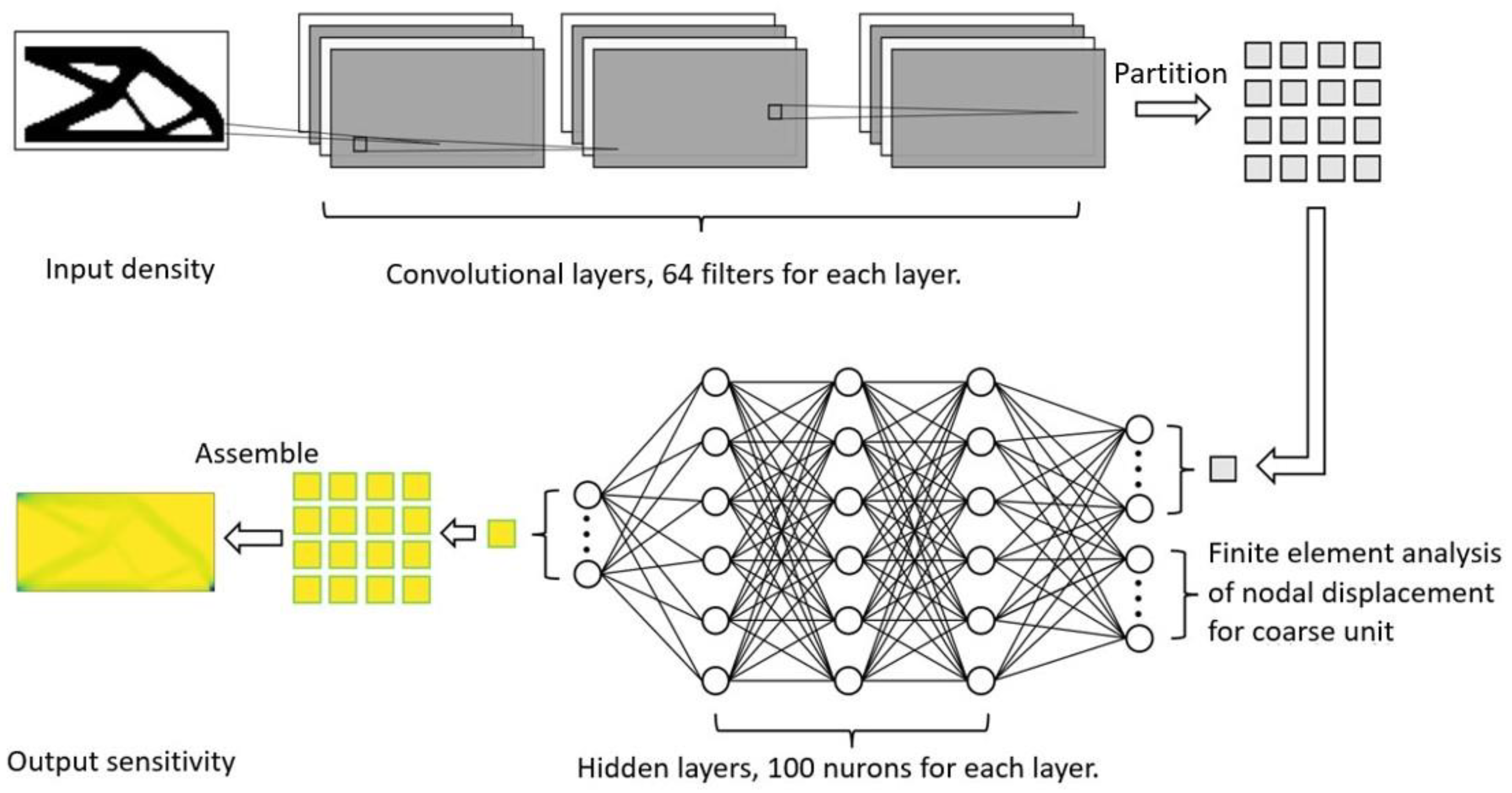
However, in most studies, using deep neural networks was not sufficiently accurate for topology optimization, mainly because it was required to perform finite element analyses of the full-scale structure at each iteration. Thus, it is necessary to improve the efficiency of finite element computation as well as the convergence of iterations during optimization. This study developed a novel partitioned deep learning algorithm to enhance structural topology optimization. The method decomposed a full-scale structure into several partitions at a coarse scale. The partition-based architecture was adopted to train the neural networks at both coarse and fine scales to reduce the computational costs of finite element analyses during topology optimization. Novel neural networks were used to optimize various types of structures of different meshes, partition numbers, and parameters. In addition, patterns of sensitivity maps were analyzed with various visualization tools to assess structural performance with high accuracy. Computational efficiency was considerably increased when the neural network technique was adopted.
The main contents of this paper are given as follows. Section 2 presents the theoretical background of the deep learning topology optimization method. Section 3 introduces the construction and training of the partitioned neural network model. Section 4 evaluates the accuracy and efficiency of neural network models in some numerical examples. Section 5 visualizes the sensitivity of neural networks with different partition numbers for several representative structures. Section 6 summarizes the contributions and limitations of this study, and points out several directions for further research in the future.

2. Theoretical Background

The idea of the surrogate-based method is to use neural networks to optimize the relationship from boundary and mesh conditions to structure density distribution. Although this type of method could maximize efficiency, the geometric connectivity might give rise to problems in the prediction results. In addition, it should be explored whether this type of method can be generalized for different types of structures. Research manuscripts reporting large datasets that are deposited in a publicly available database should specify where the data have been deposited and provide the relevant accession numbers. If the accession numbers have not yet been obtained at the time of submission, please state that they will be provided during review. They must be provided prior to publication.

2.1. Solid Isotropic Material Penalty Method

The most well-known solid isotropic material punishment (SIMP) method is adopted in this study. The density is taken as the design variable. It is gradually adjusted through iterative processes to obtain optimized configuration. Via this method, the constraint factor of the optimized structure is set from 0 to 1. The objective function and constraint conditions of the SIMP method for the minimum compliance problem are given in Equation (1).
{ min x : c ( x ) = U T K U = i = 1 N ( x e ) p u e T k 0 u e s . t . { V ( x ) V 0 = f K U = F x χ = { x n ,   0 < x min x 1 }
where F and U denote load and displacement vectors, respectively; K is the total stiffness matrix; xe is the design variable; p is the penalty factor, taken as 3 in this study; c is the overall compliance of the structure; x is the vector composed of all design variables; V0 is the volume of the initial structure; f is the percentage of the final total volume optimized by the design to the initial volume, namely, the target volume fraction; n is the total number of units in the design domain; xmin is the lower limit of the minimum density, usually taken as a non-zero minimum to prevent singular matrices in finite element computations.
The problem can be solved using several different optimization methods, such as the optimal criteria method, the sequential linear programming method, and the moving asymptotic line method. However, the optimal criterion method is used in this paper. The density update criteria are given in Equation (2).
{ max ( x min , x e m ) , x e B e η max ( x min , x e m ) x e B e η max ( x min , x e m ) x e B e η min ( 1 , x e + m ) min ( 1 , x e + m ) min ( 1 , x e + m ) x e B e η
where m denotes a positive number, limiting the range of variable changes for each iteration; η is the numerical damping coefficient taken as 1/2 in this study; Be is the density update factor, obtained from the sensitivity of each iteration, given in Equation (3).
B e = c x e λ V x e
where the Lagrange multiplier λ can be obtained by dichotomy. The sensitivity of the objective function is given in Equation (4).
c x e = p ( x e ) p 1 u e T k 0 u e
It is assumed that the derivative of the design variable with respect to volume is 1. In the optimization process, mesh dependency and a checkerboard pattern might appear. It is indicated that different grid resolutions used for optimization lead to different results. When the number of grids is increased, voids might appear in the final configuration because of grid dependency. That is, different numbers of grids might result in different topology optimization. To prevent this situation, unit density is defined as a weighted average parameter for adjacent units. The filtered unit density is written in Equations (5) and (6).
x ˜ e = 1 i N e H e i i N e H e i x i
H e i = max ( 0 , r min Δ ( e , i ) )
where Ne denotes the distance from unit e, Δ(e, i) is smaller than the filtering radius rmin of all elements; Hei is the weight factor. The weight of elements near element e is negatively correlated with the distance between two elements. The sensitivity of the ith fine-grained unit could be modified as in Equation (7).
c x e = u T K ( x e ) x e u
where u and K denote the displacement vector and stiffness matrix, respectively. Transformation from fine scale to coarse scale is given in Equation (8).
u = K 1 f = K 1 N f C = K 1 N K C u C
where superscript C denotes coarse scale, and N is loading. Thus, the sensitivity of the ith fine-grained unit can be written as in Equation (9).
c x e = ( K 1 N K C u C ) T K ( x e ) x e ( K 1 N K C u C )
The total stiffness matrices KC and K of coarse and fine grains are determined when the geometric information of the designed structure, the displacement of coarse grain structure, the distribution of the fine-grain structure, and the mapping multiple of coarse and fine grains are given. Then, the transformation matrix N is also determined. In addition, the displacement uC of coarse-grained structures is directly given in the form of input. Then, the information required to calculate the sensitivity of unit density of the objective function is obtained.

2.2. Deep Artificial Neural Networks

The behavior and function of artificial neural networks (ANNs) are determined by their network architecture. The architecture of a neural network mainly consists of several neurons among layers. In a simple fully connected neural network, the initial input layer information is first determined. Subsequently, based on the values of the input layer, the input values of the next layer of neurons are calculated through the formula written in Equation (10).
x k ( n + 1 ) = f ( i = 1 N ω i x i ( n ) + b )
where xi(n) denotes the ith neuron in the nth layer, ωi is the weight between these two layers, b is the offset between the two layers, and f(∙) is the activation function of this layer. The most commonly used activation functions are the rectified linear units (ReLU), logistic Sigmoid, and tanh functions.

2.3. Deep Learning Aided SIMP Method

The development of the first generation of computers is remarkable for their excellent computing power. The finite element method has been one of the most representative methods. In recent years, machine learning methods have made rapid progress and undergone another revolution. The goal of this study is to explore the feasibility and applicability of machine learning methods in structural optimization problems. The structural optimization problem is given in Equation (11).
( S O ) { min x , u   g 0 ( x , u ) s . t . { K ( x ) u = F ( x ) g i ( x , u ) 0 ,   i = 1 , , l x χ = { x n ,   x j min x j x j max ,   i = 1 , , n }
where K(x) is the global stiffness matrix of the structure, u is the global displacement vector, and F(x) is the global external force vector. The displacements could be written as functions of the design variables in Equation (12).
u(x) = K−1(x)F(x)
In general, the final finite element matrix form is given as K(x)u = F(x). Thus, the structural optimization problem is modified into Equation (13).
( S O ) { min x , u   g 0 ( x , u ) s . t . { a ( w h ,   v h ) = ( w h ,   f ) + ( w h ,   h ) Γ a ( w h ,   g h ) g i ( x , u ) 0 ,   i = 1 , , l x χ = { x n ,   x j min x j x j max ,   i = 1 , , n }
The surrogate-based optimization scheme is expressed in Equation (14).
( S O ) { min x , u   g 0 ( x , u ) s . t . { FEM l = 1 L g i ( x , u ) 0 ,   i = 1 , , l x χ = { x n ,   x j min x j x j max ,   i = 1 , , n }
It is indicated that the computational scheme of finite element analysis is replaced by the trained learning neural network. Displacement data are standardized in Equation (15).
u ¯ = u μ ( u ) σ ( u )
where μ(u) denotes the mean value of all displacement, and σ(u) s the variance of all displacement, which is used as the standardized input data. Because the final predicted sensitivity results may have characteristics of sparse distribution and extreme values, the coarse-grained sensitivity is used for transformation, as given in Equation (16).
s ¯ = s fine s coarse
where sfine denotes sensitivity values at fine scales, scoarse corresponds to the sensitivity of coarse mesh corresponding to fine mesh, and is the s ¯ standardized input data.

3. The Partitioned Neural Network

3.1. Schematic Diagram

The architecture of the proposed partitioned neural network scheme is shown in Figure 1. The ANN is composed of several convolutional modules. The convolution module consists of a convolution operation layer, a batch regularization layer and an activation function layer. The final convolution module outputs four feature channels. FNN consists of input layers for feature maps and coarse-grained unit node displacements, several hidden layers, and output layers representing unit sensitivity information. The activation function between hidden layers is the ReLU function. The output layer is processed by the ReLU function. Compared to traditional neural network activation functions such as logistic sigmoid and tanh hyperbolic functions, linear rectification functions have the following advantages. Firstly, linear correction and regularization can be used to adjust the activity of neurons in machine neural networks. In contrast, logic functions reach a stable state of semi saturation when the input is 0, which is not in line with the expectations of actual biology applied when simulating neural networks. Secondly, it is more efficient in gradient descent and backpropagation, and it avoids the problems of gradient explosion and vanishing. Furthermore, it simplifies the calculation process, and eliminates the influences of other complex activation functions such as exponential functions. The decentralization of activity also reduces the overall computational cost of neural networks.
To predict the sensitivity of topology optimization, cell density is essential information. A comparison between the density and sensitivity of optimization shows the spatial similarity between the two maps. The operation of the convolutional neural network (CNN) extracts relevant position features of elements in a two-dimensional matrix. It is represented in the new feature map.

3.2. Training Procedures

After several nodes are randomly selected on four boundary grid lines, displacement constraints are applied in both x and y directions. Subsequently, on other boundary grids, nodal loading is added in either the x or y direction. After the boundary conditions are set, a certain range of target volume fractions are applied. The SIMP method is used for topology optimization based on density and sensitivity. After the optimized structure is generated, the density distribution of the corresponding structure is obtained. The density of coarse-grained units is taken as the average value of corresponding fine-grained units. Subsequently, the displacement field and sensitivity map are constructed.
Next, specific training procedures are given as follows. At first, all data are distributed into specific partitions. Secondly, each batch of data is used as an input of the CNN to obtain output feature maps of several channels. Then, the output feature map is divided based on the dimensionality reduction scale, and data of each partition are transferred to ANN. The next step is to output the predictive value to calculate the error. At last, parameters of two neural networks are updated by the optimization solver based on the loss value. The previous steps are repeated for each batch of data until the entire training set is generated through specific algebra.

3.3. Verification

Figure 2 presents a simple case called the Sobel convolutional kernel. Results of scaling data and finite element computation are expressed. The unit density map and sensitivity map are given at the original scale and separated into partitions. Topology optimization iterations are randomly generated with different partitions. The time taken to complete the whole process is approximately 30 min.
To understand the impact of the number of hidden layers on the training and prediction performance of neural networks, neural networks with 10 hidden layers are trained. The CNN filter size is set to 64, and the hidden layer neurons number 100. The loss function curve for the training of the network is shown in Figure 3. It is indicated that the decline of the error gets smaller. The partitioned network consisting of 10 layers of CNN is selected for the experiment among neural networks with 20, 50, 100, 200, 300, and 400 hidden layer neurons, respectively. After 100 generations of training, the result of the training dataset is shown in Figure 4. Next, preliminary training is conducted on the neural network using a random dataset. Figure 4 shows that the loss function value rapidly decreases before 20 steps during the training process. At around 20 steps, the deceleration tends to ease. At 80 steps, it almost converges. However, there was a certain degree of oscillation throughout the entire process. The predicted results of the training model are compared with the experimental results, as shown in Figure 5. Figure 5a presents the fine scale structure density map. Figure 5b shows the difference between results from SIMP with and without ANN. It is indicated that the solutions of the training model are in good agreement with the experimental results. However, ANN obtains both convolutional features and displacement input from finite element computation. Displacement data have a sparse distribution and individual extreme values.

4. Numerical Examples

In this section, the proposed artificial neural network method is used to perform topology optimization for some numerical examples such as the cantilever beam, the MBB beam, the L-shape beam, the column, and the rod-supported bridge. The tool of visualization used in this study is Visio. Visio is fully functional and easy to learn, supporting the creation of various types of diagrams, including network topology diagrams. It is suitable for various application scenarios, but is mainly used for chart design and does not have professional topology management functions. Details of the numerical experiments are given as follows.

4.1. The Cantilever Beam

One numerical experiment is performed for the cantilever beam with 60 × 60 meshes under concentrated loading at the middle of the right end in this section. The structure is generated with the target volume fraction Vf of 0.2 and a density filter radius rmin of 1.5, and 20 optimization iteration steps. Figure 6 presents boundary conditions and topological configuration of the cantilever beam.

4.2. The MBB Beam

Another numerical experiment is performed for the MBB beam with 360 × 120 meshes under concentrated loading on the top of the left end in this section. The structure is generated with the target volume fraction Vf of 0.2 and a density filter radius rmin of 1.5, and the optimization iteration steps are set at 20. Figure 7 reveals the boundary conditions and topological configuration of the MBB beam.

4.3. The L-Shape Beam

Another numerical experiment is performed on an L-shaped beam with 240 × 240 meshes under concentrated loading on the top of the right end in this section. The structure is generated with the target volume fraction Vf of 0.2 and a density filter radius rmin of 1.5. The optimization iteration steps are set at 20. Figure 8 unveils the boundary conditions and topological configuration of the L-shaped beam.

4.4. The Column

A numerical experiment is performed for the column with 240 × 240 meshes under distributed loading on the top in this section. The structure is generated with the target volume fraction Vf of 0.2 and a density filter radius rmin of 1.5. The optimization iteration steps are set at 20. Figure 9 presents the boundary conditions and topological configuration of the column.

4.5. The Rod Supported Bridge

A numerical experiment is performed for a rod-supported bridge with 240 × 240 meshes under distributed loading on the top in this section. The structure is generated with the target volume fraction Vf of 0.2 and a density filter radius rmin of 1.5. The optimization iteration steps are set at 20. Figure 10 displays the boundary conditions and topological configuration of the rod-supported bridge.

5. Results and Discussion

Comparing two multi-objective meta-heuristic algorithms involves several steps to ensure a comprehensive and fair evaluation. Here are some of the best practices and metrics to consider. First of all, clearly specify the objectives that the algorithms aim to optimize. This could include maximizing/minimizing multiple conflicting objectives. Secondly, select a diverse set of benchmark problems that are widely used in the literature for multi-objective optimization. These problems should vary in complexity, dimensionality, and characteristics. Then, choose appropriate performance metrics to evaluate the algorithms. Common metrics include convergence metrics, measurement of the volume of the objective space covered by the Pareto front, evaluation of the distance from a set of solutions to the true Pareto front, and assessment of how well the solutions cover the Pareto front. Next, ensure both algorithms are properly tuned for their parameters to guarantee a fair comparison. Run each algorithm multiple times to account for stochasticity in results. Use statistical tests to analyze the significance of the results. In addition, use statistical methods to analyze the performance of the algorithms. Common approaches include Wilcoxon rank-sum test, analysis of variance, and effect size measures. Also, graphical representations help in understanding the performance visually, such as Pareto front visualization, boxplots, and convergence plots. Furthermore, evaluate the robustness of the algorithms by testing them on different problem instances or varying conditions. Finally, measure and compare the computational time and resources required by each algorithm to reach the results. This includes execution time and memory usage. If applicable, consider any specific characteristics of the problem domain that may impact the performance or suitability of the algorithms. In general, a thorough comparison involves a combination of quantitative metrics, statistical analysis, visual representation, and consideration of robustness and computational efficiency. This holistic approach ensures that the strengths and weaknesses of each algorithm are well understood, leading to informed conclusions about their relative performances.

5.1. Convergency

The SIMP method is used for the numerical examples given in the previous section. The decline of the optimization objective functions is shown in Figure 11. It is indicated that most of them reach convergence from 10 to 20 steps, although the rate of convergence of random structures is different.
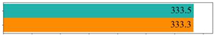
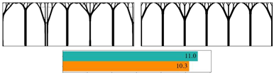
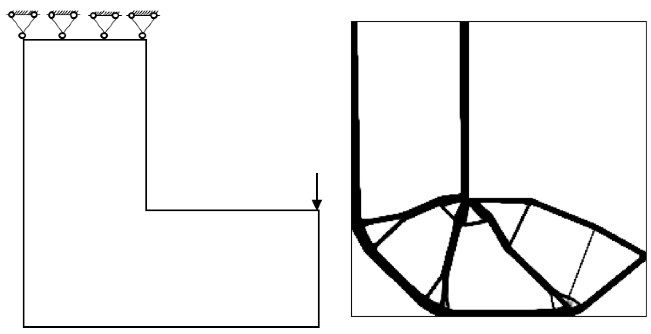
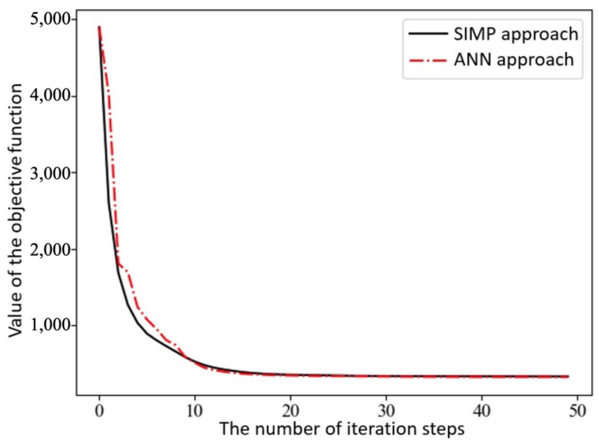
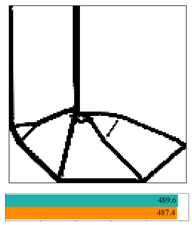
The final convergent values of the objective function using the partitioned deep learning algorithm-aided optimization method newly developed in this paper are similar. Figure 12 made a comparison between iterative objective functions of SIMP and ANN.

5.2. Effect of Partition Number on Optimization

Table 1, Table 2 and Table 3 list the neural network prediction results for three different grid numbers and two block dimensions, where sensitivity filters with a radius of 4 are applied to all cases with a partition number Np = 3.
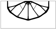
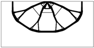
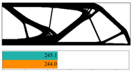
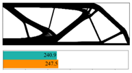
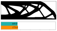
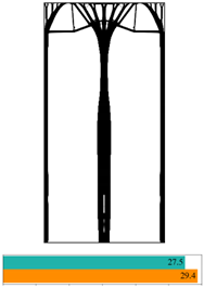
It is demonstrated that the proposed method can be generalized to different cases. That is, the method is applicable for different target volume fractions and filtering radii. More numerical examples and experiments are given in Appendix A.

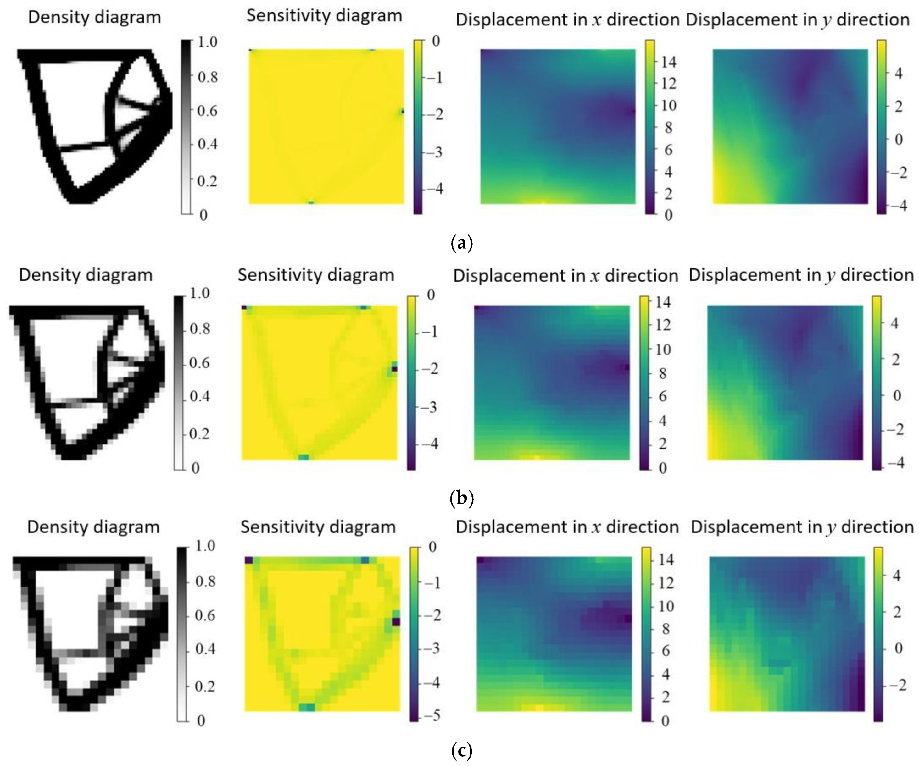
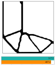
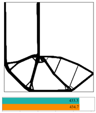
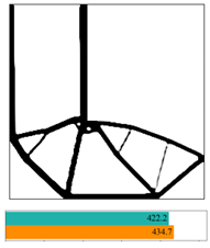
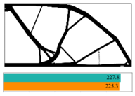
5.3. Effect of Topology Optimization Parameter on Optimization

Table 4, Table 5 and Table 6 compare the previous numerical examples with various target volume fractions and filtering radii. It is indicated that sensitivity is independent of the target volume fraction, density filtering radius and other parameters of topology optimization. More numerical examples and experiments are given in Appendix A.

5.4. Proportion of FEA Time Consumption

Next, the proportion of FEA time consumption in the entire process of SIMP and ANN methods is investigated. The main source of consumption in finite element calculation is the sparse matrix equation solver. The computational cost in other steps is represented by the density updating of the optimization solver. The test results are shown in Figure 13.
It is demonstrated that the finite element computation takes more than 90% of the total operation time of the SIMP method. This result is in good agreement with one obtained by Mukherjee et al. [
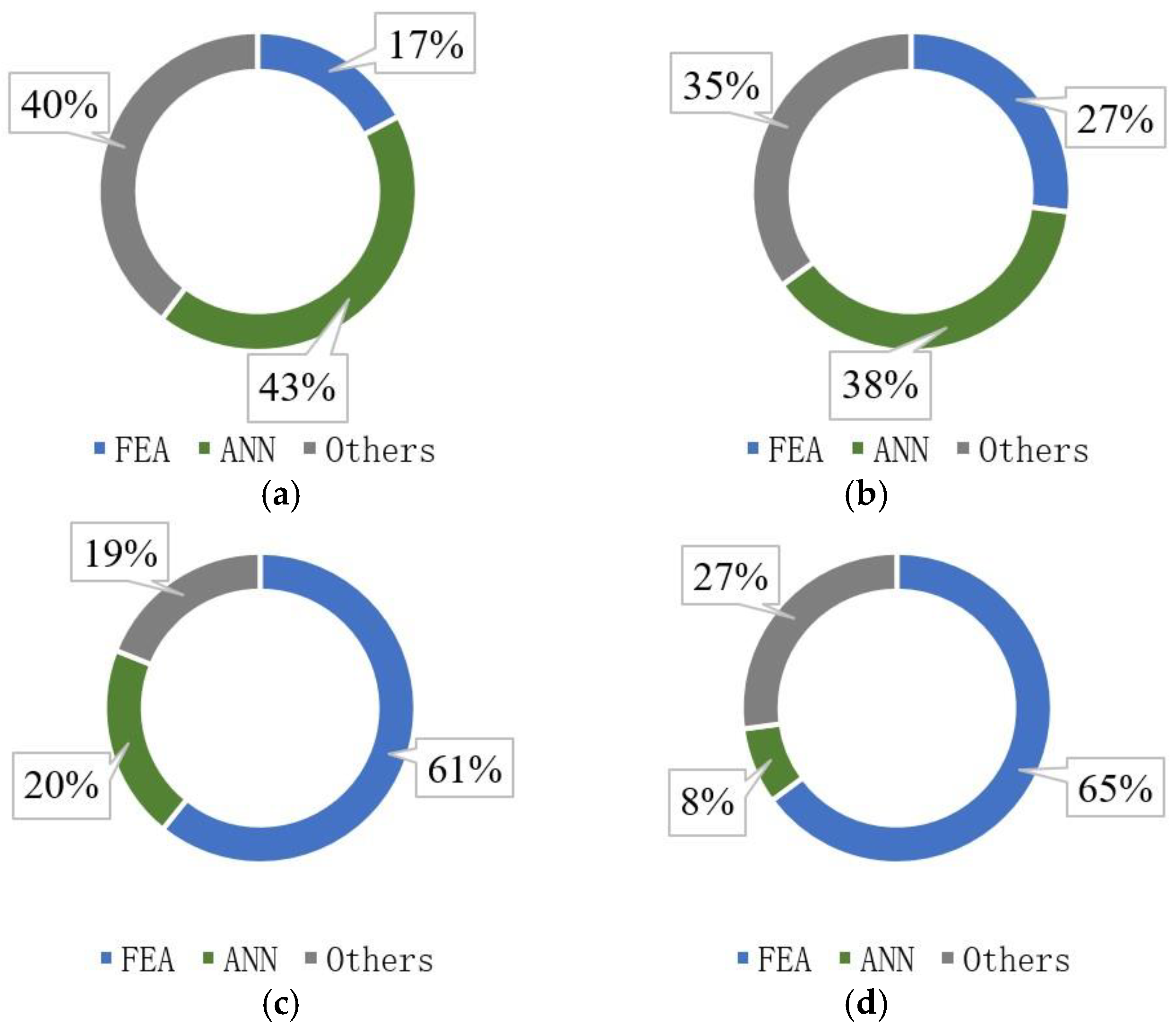
5]. Also, the proportion represented by running time in finite element computations via neural network methods with different partitions and different design variables is explored, as shown in
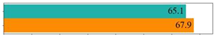
 Figure 14.
It is observed that the computational cost and ratio of finite element method are lower than those of traditional SIMP method. The larger the dimension of partitioning is, the smaller the computational cost and proportion of finite element analysis are. It is indicated that the proposed technique effectively alleviates excessive works of finite element computation during topology optimization. In addition, as the number of structural grids increases, the time proportion of neural network inference in the entire process gradually decreases. It is inferred that under the condition of millions of elements, as are seen in actual application scenarios, the additional computational consumption of neural network prediction can be ignored. That is, using neural network methods to enhance large-scale structural topology optimization is feasible.

6. Conclusions

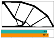
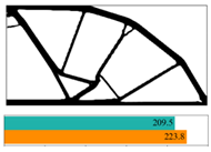
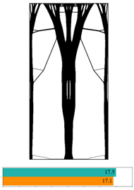
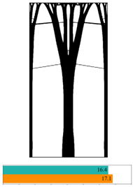
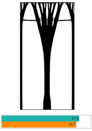
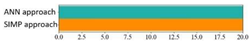
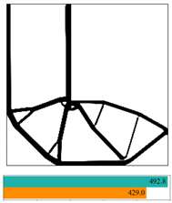
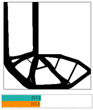
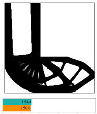
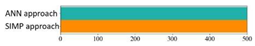
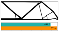
This study proposes a partitioned deep learning algorithm to aid structural topology optimization. The main conclusions obtained from this study are summarized as follows. First, in the training phase of neural networks, it is found that using random structural training datasets significantly improves the prediction accuracy of neural networks for different structures. The larger the size of the training dataset is, the higher the prediction accuracy is. In addition, selecting several steps of data training in the early stage of iteration convergence results in a high prediction accuracy for the model. Also, it is demonstrated that the smaller the size of partition is, the better the training result is. Secondly, the topology configuration obtained from the novel approach is similar to that derived using the SIMP method. The difference in structural performance between the two approaches is less than 10%. Also, compared with the SIMP method, the neural network method of structural optimization significantly increases computational efficiency. As the number of partitions in the neural network further increases, the difference in cost proportion when fully using finite element computation further increases.
However, this study only investigated a small number of partitions. That is, it is possible that the generalization performance could be improved using neural networks only for simple problems. In addition, in this study, only two-dimensional plane stress problems were considered. Further explorations into the use of the proposed method in three-dimensional complex structures with large numbers of partitions will be necessary in the future.

Author Contributions

Conceptualization, X.K. and Y.W.; methodology, X.K.; resources and data curation, Q.Y. and P.Z. (Peng Zhu); software, P.Z. (Peng Zhi); validation, Q.Y. and X.K.; formal analysis, X.K.; investigation, X.K. writing—original draft preparation, X.K.; writing—review and editing, Y.W.; visualization, X.K.; supervision, P.Z. (Peng Zhu); project administration, Y.W.; funding acquisition, Y.W. All authors have read and agreed to the published version of the manuscript.

Funding

This research was funded by the National Natural Science Foundation of China, grant number 52178299.

Institutional Review Board Statement

Not applicable.

Informed Consent Statement

Not applicable.

Data Availability Statement

The original contributions presented in this study are included in the article. Further inquiries can be directed to the corresponding authors.

Acknowledgments

The authors wish to thank Jesus Christ for listening to our prayers and the anonymous reviewers for their thorough review of this article and their constructive advice.

Conflicts of Interest

The authors declare no conflicts of interest.

Appendix A

For the sake of comparison, structural topology optimizations of more numerical examples are made using the proposed artificial neural network approach and conventional SIMP method, as shown in Table A1.
Table A1. Structural topology optimizations of 25 numerical examples.
Structure StyleBoundary and Loading Methodology
ANN Applsci 14 11416 i001SIMP Applsci 14 11416 i002
Cantilever beamApplsci 14 11416 i003Applsci 14 11416 i004Applsci 14 11416 i005
Applsci 14 11416 i006
Two-node constrained beamApplsci 14 11416 i007Applsci 14 11416 i008Applsci 14 11416 i009
Applsci 14 11416 i010
1/2 canyon BridgeApplsci 14 11416 i011Applsci 14 11416 i012Applsci 14 11416 i013
Applsci 14 11416 i014
1/3 low approach bridgeApplsci 14 11416 i015Applsci 14 11416 i016
Applsci 14 11416 i017
1/3 middle approach bridgeApplsci 14 11416 i018Applsci 14 11416 i019
Applsci 14 11416 i020
1/3 high approach bridgeApplsci 14 11416 i021Applsci 14 11416 i022
Applsci 14 11416 i023
1/2 load-bearing columnApplsci 14 11416 i024Applsci 14 11416 i025Applsci 14 11416 i026
Applsci 14 11416 i027
CraneApplsci 14 11416 i028Applsci 14 11416 i029Applsci 14 11416 i030
Applsci 14 11416 i031
DamApplsci 14 11416 i032Applsci 14 11416 i033Applsci 14 11416 i034
Applsci 14 11416 i035
Suspension bridgeApplsci 14 11416 i036Applsci 14 11416 i037Applsci 14 11416 i038
Applsci 14 11416 i039
1/2 suspension structureApplsci 14 11416 i040Applsci 14 11416 i041Applsci 14 11416 i042
Applsci 14 11416 i043
1/2 cyclic structureApplsci 14 11416 i044Applsci 14 11416 i045Applsci 14 11416 i046
Applsci 14 11416 i047
Thin L-shaped beamApplsci 14 11416 i048Applsci 14 11416 i049Applsci 14 11416 i050
Applsci 14 11416 i051
Thick L-shaped beamApplsci 14 11416 i052Applsci 14 11416 i053Applsci 14 11416 i054
Applsci 14 11416 i055
1/2 MBB beamApplsci 14 11416 i056Applsci 14 11416 i057
Applsci 14 11416 i058
1/2 Michell beamApplsci 14 11416 i059Applsci 14 11416 i060Applsci 14 11416 i061
Applsci 14 11416 i062
1/2 Michell beamApplsci 14 11416 i063Applsci 14 11416 i064Applsci 14 11416 i065
Applsci 14 11416 i066
1/2 multi-story structureApplsci 14 11416 i067Applsci 14 11416 i068Applsci 14 11416 i069
Applsci 14 11416 i070
1/2 pure bending moment beamApplsci 14 11416 i071Applsci 14 11416 i072Applsci 14 11416 i073
Applsci 14 11416 i074
SlopeApplsci 14 11416 i075Applsci 14 11416 i076Applsci 14 11416 i077
Applsci 14 11416 i078
1/3 roofApplsci 14 11416 i079Applsci 14 11416 i080
StaircaseApplsci 14 11416 i081Applsci 14 11416 i082Applsci 14 11416 i083
Applsci 14 11416 i084
1/2 suspension bridgeApplsci 14 11416 i085Applsci 14 11416 i086
1/3 supported bridgeApplsci 14 11416 i087Applsci 14 11416 i088
1/3 double deck bridgeApplsci 14 11416 i089Applsci 14 11416 i090

References

  1. Genovese, F.; Alderucci, T.; Muscolino, G. Design sensitivity analysis of structural systems with damping devices subjected to fully non-stationary stochastic seismic excitations. Comput. Struct. 2023, 284, 107067. [Google Scholar] [CrossRef]
  2. Khatir, A.; Capozucca, R.; Khatir, S.; Magagnini, E. Vibration-based crack prediction on a beam model using hybrid butterfly optimization algorithm with artificial neural network. Front. Struct. Civ. Eng. 2022, 16, 976–989. [Google Scholar] [CrossRef]
  3. Carbas, S.; Artar, M. Comparative seismic design optimization of spatial steel dome structures through three recent metaheuristic algorithms. Front. Struct. Civ. Eng. 2022, 16, 57–74. [Google Scholar] [CrossRef]
  4. Wang, X.; Wu, J.; Yin, X.; Liu, Q.; Huang, X.; Pan, Y.; Yang, J.; Huang, L.; Miao, S. QPSO-ILF-ANN-based optimization of TBM control parameters considering tunneling energy efficiency. Front. Struct. Civ. Eng. 2023, 17, 25–36. [Google Scholar] [CrossRef]
  5. Vantyghem, G.; De Corte, W.; Shakour, E. 3D printing of a post-tensioned concrete girder designed by topology optimization. Autom. Constr. 2020, 112, 103084. [Google Scholar] [CrossRef]
  6. Mukherjee, S.; Lu, D.; Raghavan, B. Accelerating large-scale topology optimization: State-of-the-art and challenges. Arch. Comput. Methods Eng. 2021, 28, 4549–4571. [Google Scholar] [CrossRef]
  7. Bendsøe, M.P.; Kikuchi, N. Generating optimal topologies in structural design using a homogenization method. Comput. Methods Appl. Mech. Eng. 1988, 71, 197–224. [Google Scholar] [CrossRef]
  8. Zhou, M.; Rozvany, G. The COC algorithm, Part II: Topological, geometry and generalised shape optimisation. Comput. Methods Appl. Mech. Eng. 1991, 89, 309–336. [Google Scholar] [CrossRef]
  9. Bendsøe, M.P.; Sigmund, O. Material interpolation schemes in topology optimization. Arch. Appl. Mech. 1999, 69, 635–654. [Google Scholar] [CrossRef]
  10. Yang, X.; Xie, Y.; Steven, G. Bidirectional evolutionary method for stiffness optimization. AIAA J. 1999, 37, 1483–1488. [Google Scholar] [CrossRef]
  11. Huang, X.; Xie, Y. Convergent and mesh-independent solutions for the bi-directional evolutionary structural optimization method. Finite Elem. Anal. Des. 2007, 43, 1039–1049. [Google Scholar] [CrossRef]
  12. Allaire, G.; Jouve, F.; Toader, A.-M. A level-set method for shape optimization. Comput. Rendus Math. 2002, 334, 1125–1130. [Google Scholar] [CrossRef]
  13. Allaire, G.; Jouve, F.; Toader, A.-M. Structural optimization using sensitivity analysis and a level-set method. J. Comput. Phys. 2004, 194, 363–393. [Google Scholar] [CrossRef]
  14. Wang, M.Y.; Wang, X.; Guo, D. A level set method for structural topology optimization. Comput. Methods Appl. Mech. Eng. 2003, 192, 227–246. [Google Scholar] [CrossRef]
  15. Bourdin, B.; Chambolle, A. Design-dependent loads in topology optimization. ESAIM: Control Optim. Calc. Var. 2003, 9, 19–48. [Google Scholar] [CrossRef]
  16. Guo, X.; Zhang, W.; Zhong, W. Doing topology optimization explicitly and geometrically—A new moving morphable components based framework. J. Appl. Mech. 2014, 81, 081009. [Google Scholar] [CrossRef]
  17. Guo, X.; Zhang, W.; Zhang, J. Explicit structural topology optimization based on moving morphable components (MMC) with curved skeletons. Comput. Methods Appl. Mech. Eng. 2016, 310, 711–748. [Google Scholar] [CrossRef]
  18. Zhang, W.; Chen, J.; Zhu, X. Explicit three-dimensional topology optimization via Moving Morphable Void (MMV) approach. Comput. Methods Appl. Mech. Eng. 2017, 322, 590–614. [Google Scholar] [CrossRef]
  19. Zhang, W.; Yang, W.; Zhou, J. Structural topology optimization through explicit boundary evolution. J. Appl. Mech. 2017, 84, 011011. [Google Scholar] [CrossRef]
  20. Eschenauer, H.A.; Kobelev, V.V.; Schumacher, A. Bubble method for topology and shape optimization of structures. Struct. Optim. 1994, 8, 42–51. [Google Scholar] [CrossRef]
  21. Cai, S.; Zhang, W. An adaptive bubble method for structural shape and topology optimization. Comput. Methods Appl. Mech. Eng. 2020, 360, 112778. [Google Scholar] [CrossRef]
  22. Woldseth, R.V.; Aage, N.; Bærentzen, J.A. On the use of artificial neural networks in topology optimisation. Struct. Multidiscip. Optim. 2022, 65, 294. [Google Scholar] [CrossRef]
  23. Bolandi, H.; Li, X.; Salem, T.; Boddeti, V.N.; Lajnef, N. Bridging finite element and deep learning: High-resolution stress distribution prediction in structural components. Front. Struct. Civ. Eng. 2022, 16, 1365–1377. [Google Scholar] [CrossRef]
  24. Teng, S.; Chen, G.; Wang, S.; Zhang, J.; Sun, X. Digital image correlation-based structural state detection through deep learning. Front. Struct. Civ. Eng. 2022, 16, 45–56. [Google Scholar] [CrossRef]
  25. Wu, X.; Li, J.; Wang, L. Efficient Identification of water conveyance tunnels siltation based on ensemble deep learning. Front. Struct. Civ. Eng. 2022, 16, 564–575. [Google Scholar] [CrossRef]
  26. Yang, Y.F.; Liao, S.M.; Liu, M.B. Dynamic prediction of moving trajectory in pipe jacking: GRU-based deep learning framework. Front. Struct. Civ. Eng. 2023, 17, 994–1010. [Google Scholar] [CrossRef]
  27. Goodfellow, I.; McDaniel, P.; Papernot, N. Making machine learning robust against adversarial inputs. Commun. ACM 2018, 61, 56–66. [Google Scholar] [CrossRef]
  28. Morrison, O.M.; Pichi, F.; Hesthaven, J.S. GFN: A graph feedforward network for resolution-invariant reduced operator learning in multifidelity applications. arXiv 2024, arXiv:2406.03569. [Google Scholar] [CrossRef]
  29. Valentino, C.; Pagano, G.; Conte, D.; Paternoster, B.; Colace, F.; Casillo, M. Step-by-step time discrete Physics-Informed Neural Networks with application to a sustainability PDE model. Math. Comput. Simul. 2024, in press. [Google Scholar] [CrossRef]
  30. Zheng, S.; Fan, H.; Zhang, Z. Accurate and real-time structural topology prediction driven by deep learning under moving morphable component-based framework. Appl. Math. Model. 2021, 97, 522–535. [Google Scholar] [CrossRef]
  31. Hoang, V.N.; Nguyen, N.L.; Tran, D.Q.; Vu, Q.-V.; Nguyen-Xuan, H. Data-driven geometry-based topology optimization. Struct. Multidiscip. Optim. 2022, 65, 69. [Google Scholar] [CrossRef]
  32. Kaveh, A.; Bahreininejad, A.; Mostafaie, M. A hybrid graph-neural method for domain decomposition. Comput. Struct. 1999, 70, 667–674. [Google Scholar]
  33. Kaveh, A.; Servati, H. Design of double layer grids using back-propagation neural networks. Comput. Struct. 2001, 79, 1561–1568. [Google Scholar] [CrossRef]
  34. Kaveh, A.; Raiessi, D.M. RBF and BP neural networks for the analysis and design of domes. Int. J. Space Struct. 2003, 18, 181–194. [Google Scholar] [CrossRef]
  35. Iranmanesh, A.; Kaveh, A. Structural optimization by gradient base neural networks. Int. J. Numer. Methods Eng. 1999, 46, 297–311. [Google Scholar] [CrossRef]
  36. Kaveh, A.; Dadras, A.; Geran, M.N. Robust design optimization of laminated plates under uncertain bounded buckling loads. Struct. Multidiscip. Optim. 2018, 59, 877–891. [Google Scholar] [CrossRef]
  37. Kaveh, A.; Kalateh-Ahani, M.; Fahimi-Farzam, M. Constructability optimal design of reinforced concrete retaining walls using a multi-objective genetic algorithm. Struct. Eng. Mech. 2013, 47, 227–245. [Google Scholar] [CrossRef]
  38. Kaveh, A.; Laknejadi, K. A novel hybrid charge system search and particle swarm optimization method for multi-objective optimization. Expert Syst. Appl. 2011, 38, 15475–15488. [Google Scholar] [CrossRef]
  39. Zheng, S.; He, Z.; Liu, H. Generating three-dimensional structural topologies via a U-Net convolutional neural network. Thin-Walled Struct. 2021, 159, 107263. [Google Scholar] [CrossRef]
  40. Lei, X.; Liu, C.; Du, Z. Machine learning-driven real-time topology optimization under moving morphable component-based framework. J. Appl. Mech. 2019, 86, 011004. [Google Scholar] [CrossRef]
  41. Yu, Y.; Hur, T.; Jung, J. Deep learning for determining a near-optimal topological design without any iteration. Struct. Multidiscip. Optim. 2019, 59, 787–799. [Google Scholar] [CrossRef]
  42. Nakamura, K.; Suzuki, Y. Deep learning-based topological optimization for representing a user-specified design area. arXiv 2020, arXiv:2004.05461. [Google Scholar]
  43. Luo, J.; Li, Y.; Zhou, W. An Improved Data-Driven Topology Optimization Method Using Feature Pyramid Networks with Physical Constraints. CMES-Comput. Model. Eng. Sci. 2021, 128, 823–848. [Google Scholar] [CrossRef]
  44. Behzadi, M.M.; Ilies, H.T. GANTL: Towards practical and real-time topology optimization with conditional GANs and transfer learning. J. Mech. Des. 2022, 144, 021711. [Google Scholar] [CrossRef]
  45. Raissi, M.; Perdikaris, P.; Karniadakis, G.E. Physics-informed neural networks: A deep learning framework for solving forward and inverse problems involving nonlinear partial differential equations. J. Comput. Phys. 2019, 378, 686–707. [Google Scholar] [CrossRef]
  46. Lu, L.; Jin, P.; Pang, G. Learning nonlinear operators via DeepONet based on the universal approximation theorem of operators. Nat. Mach. Intell. 2021, 3, 218–229. [Google Scholar] [CrossRef]
  47. Chi, H.; Zhang, Y.; Tang, T.L.E. Universal machine learning for topology optimization. Comput. Methods Appl. Mech. Eng. 2021, 375, 112739. [Google Scholar] [CrossRef]
  48. Zhang, Y.; Chi, H.; Chen, B. Speeding up Computational Morphogenesis with Online Neural Synthetic Gradients. International Joint Conference on Neural Networks. arXiv 2021, arXiv:2104.12282. [Google Scholar]
  49. Qian, C.; Ye, W. Accelerating gradient-based topology optimization design with dual-model artificial neural networks. Struct. Multidiscip. Optim. 2021, 63, 1687–1707. [Google Scholar] [CrossRef]
  50. Tan, R.K.; Qian, C.; Xu, D. An Adaptive and Scalable ANN-based Model-Order-Reduction Method for Large-Scale TO Designs. arXiv 2022, arXiv:2203.10515. [Google Scholar]
  51. Yue, T.; Yang, H.; Du, Z. A mechanistic-based data-driven approach to accelerate structural topology optimization through finite element convolutional neural network (FE-CNN). arXiv 2021, arXiv:2106.13652. [Google Scholar]
  52. Nguyen, T.H.; Paulino, G.H.; Song, J. Improving multiresolution topology optimization via multiple discretizations. Int. J. Numer. Methods Eng. 2012, 92, 507–530. [Google Scholar] [CrossRef]
  53. Groen, J.P.; Langelaar, M.; Sigmund, O. Higher-order multi-resolution topology optimization using the finite cell method. Int. J. Numer. Methods Eng. 2017, 110, 903–920. [Google Scholar] [CrossRef]
  54. Kallioras, N.A.; Kazakis, G.; Lagaros, N.D. Accelerated topology optimization by means of deep learning. Struct. Multidiscip. Optim. 2020, 62, 1185–1212. [Google Scholar] [CrossRef]
Figure 1. Schematic diagram of partitioned neural network architecture.
Applsci 14 11416 g001
Figure 2. Density, sensitivity, and displacement maps of sample structures at different partitions, (a) 60 × 60, (b) 30 × 30, and (c) 20 × 20.
Applsci 14 11416 g002
Figure 3. Descent of loss function of neural networks with (a) 5 and (b) 10 hidden layers.
Applsci 14 11416 g003
Figure 4. Training loss function descent history.
Applsci 14 11416 g004
Figure 5. (a) Fine-scale structure density map; (b) difference between results from SIMP with and without ANN.
Applsci 14 11416 g005
Figure 6. Boundary conditions and topological configuration of the cantilever beam with 60 × 60 mesh loaded at the middle of the right end.
Applsci 14 11416 g006
Figure 7. Boundary conditions and topological configuration of the MBB beam with 360 × 120 mesh.
Applsci 14 11416 g007
Figure 8. Boundary conditions and topological configuration of the L-shaped beam with 240 × 240 meshes.
Applsci 14 11416 g008
Figure 9. Boundary conditions and topological configuration of the 1/3 column with 240 × 240 meshes.
Applsci 14 11416 g009
Figure 10. Boundary conditions and topological configuration of the 1/3 rod-supported bridge with 240 × 240 mesh.
Applsci 14 11416 g010
Figure 11. The descent history of the objective function for five numerical examples.
Applsci 14 11416 g011
Figure 12. Comparison between iterative objective functions of SIMP and ANN.
Applsci 14 11416 g012
Figure 13. The proportion of time consumption for each module of the SIMP method with (a) 60 × 60, (b) 120 × 120, (c) 240 × 240, and (d) 480 × 480 meshes.
Applsci 14 11416 g013
Figure 14. The proportion of time consumption of each module in the neural network method for 3×3 partitioned structure with (a) 60 × 60, (b) 120 × 120, (c) 240 × 240, and (d) 480 × 480 meshes.
Applsci 14 11416 g014
Table 1. Comparison among L-shaped beams with different partition numbers.
MeshNp = 2Np = 3
120 × 120Applsci 14 11416 i091Applsci 14 11416 i092
240 × 240Applsci 14 11416 i093Applsci 14 11416 i094
480 × 480Applsci 14 11416 i095Applsci 14 11416 i096
Applsci 14 11416 i097
Table 2. Comparison among MBB beams with different partition numbers.
MeshNb = 2Nb = 3
240 × 120Applsci 14 11416 i098Applsci 14 11416 i099
360 × 180Applsci 14 11416 i100Applsci 14 11416 i101
480 × 240Applsci 14 11416 i102Applsci 14 11416 i103
Applsci 14 11416 i104
Table 3. Comparison among columns with different partition numbers.
MeshNp = 2Np = 3
120 × 480Applsci 14 11416 i105Applsci 14 11416 i106
180 × 720Applsci 14 11416 i107Applsci 14 11416 i108
240 × 960Applsci 14 11416 i109Applsci 14 11416 i110
Applsci 14 11416 i111
Table 4. The predicted results of the L-beams (240 × 240) with different topology optimization parameters.
Vfrmin = 2rmin = 3rmin = 4
0.2Applsci 14 11416 i112Applsci 14 11416 i113Applsci 14 11416 i114
0.4Applsci 14 11416 i115Applsci 14 11416 i116Applsci 14 11416 i117
0.6Applsci 14 11416 i118Applsci 14 11416 i119Applsci 14 11416 i120
Applsci 14 11416 i121
Table 5. The predicted results of the MBB beams (320 × 120) with different topology optimization parameters.
Vfrmin = 2rmin = 3rmin = 4
0.2Applsci 14 11416 i122Applsci 14 11416 i123Applsci 14 11416 i124
0.4Applsci 14 11416 i125Applsci 14 11416 i126Applsci 14 11416 i127
0.6Applsci 14 11416 i128Applsci 14 11416 i129Applsci 14 11416 i130
Applsci 14 11416 i131
Table 6. The predicted results of the columns (120 × 480) with different topology optimization parameters.
Vfrmin = 2rmin = 3rmin = 4
0.2Applsci 14 11416 i132Applsci 14 11416 i133Applsci 14 11416 i134
0.3Applsci 14 11416 i135Applsci 14 11416 i136Applsci 14 11416 i137
0.4Applsci 14 11416 i138Applsci 14 11416 i139Applsci 14 11416 i140
Applsci 14 11416 i141
Disclaimer/Publisher’s Note: The statements, opinions and data contained in all publications are solely those of the individual author(s) and contributor(s) and not of MDPI and/or the editor(s). MDPI and/or the editor(s) disclaim responsibility for any injury to people or property resulting from any ideas, methods, instructions or products referred to in the content.

