Water Demand (or Specific Surface) of Aggregate as a Dominating Factor for SCC Composition Design

Abstract

In the modern era of superplasticizer-based concrete technology, water demand (or specific surface) of aggregate is a significantly underestimated factor influencing cement paste demand in the self-compacting concrete (SCC) design process. The presented data show that it is the key factor for optimization criterion of SCC cement paste demand. Four models were taken into consideration (Bolomey, Stern, modified Loudon, and Relative Specific Surface), and all of them fit linearly very well (R² ≥ 0.95) to the relative thickness of coating aggregate with cement paste (t_rel). This means that all of these models may be used interchangeably in the process of SCC design without any alteration (so there is no need to develop a new model). Including the water demand of aggregate in the design procedure in its proposed version sets the bottom limit of superplasticizer dose for laboratory trials, leaving only small gap for eventual minor adjustments.

1. Introduction

Self-compacting concrete (SCC) has been known for about 30 years, but its composition design is still a serious technical problem: in the works [1,2,3,4,5] over 60 methods of composition design of SCC have been collected (till 2018). Due to the application nature of this publication, the literature query is deliberately limited. All examples given below have been deliberately selected from the entire 30-year period of SCC use (also newer ones than those mentioned in Refs. [1,2,3,4,5]), usually citing 3 characteristic methods illustrating a given phenomenon or feature.

Such a wide spectrum of reported design methods indicates, on the one hand, great research interest in this regard. On the other hand, however, it indicates a lack of agreement on the basic rules governing self-compacting ability. As an example, one can give the simplest and probably most obvious distinguishing factor regarding the selection of aggregate composition for SCC: whether the aggregate should be composed assuming its compacted or loose state as the basis. The cited methods are divided in this respect roughly 50:50. Thus, half of them are based on the traditional method transferred directly from normal fluidity concretes (e.g., all methods described in Ref. [2]; modern examples: Refs. [6,7,8]). The second half is based on the assumption of a loose state formulated for the first time in Ref. [9]; other examples can be found in Refs. [3,10].

It should not be forgotten that the universal application of a given technical solution is always the ultimate goal of all scientific research in the field of building industry. That is why there is a fundamental question, unfortunately basically rhetorical: which methods are used by designers of SCC mixtures for industry. In this respect, the author is not aware of any comprehensive source data. In general, in engineering practice, it is easiest to rely on something already known which only needs to be modified in some way—see for instance an interesting attempt to adopt the standard ACI method [11]. Therefore, the author has decided to base his own research on the Polish laboratory method of designing a traditional concrete mix according to Kuczyński [12]. The method of determining the aggregate composition described in Ref. [3] was adopted from this method. In the further development of the method, it turned out [13,14] that the minimum paste content necessary to achieve self-compacting ability (V_{paste min}) depends on the specific surface area determined by the method of Oh et al. [15]. This observation is somewhat “against the flow” of the main trends in SCC design, as only four other methods are based on this assumption [9,15,16,17]. The rest of methods are based on:

• The voids of the aggregate (overfilling or paste/mortar thickness methods), e.g., [17,18,19] etc.;
• The packing of particles (CPM method [20] and its modern derivatives, e.g., [7,8] etc.);
• Blocking criterion for obtaining good passing ability, e.g., [21,22] etc.;
• Nomograms or fixed aggregate content, e.g., [21,23,24], the UCI method [2,5] and its derivatives—e.g., [25]—etc.

Therefore, specific surface of aggregate assessment for a SCC composition design is generally underestimated. Neglecting specific surface of aggregate in SCC design is based on the use of super-efficient superplasticizers (SP) based on polycarboxylates. In the case of the occurrence of problems resulting from the greater water demand of the granular phase, typically it is enough to use more admixture. This approach is proposed in almost all cited SCC design methods. It results from the tendency of use of high dosages of fine-grained additions in SCC composition. In such a case, paste phase water demand dominates the water demand of the aggregate. Unfortunately, the approach requires troublesome adjustment of the SP content on the test mixtures and results in obtaining not always satisfactory (i.e., too high) paste content.

That is why the natural next step in development of our own method is to check whether other existing simple methods of water demand/specific surface calculation are also suitable for this purpose. This is also a “remake” of old Polish analytical method of traditional concrete design, called “three equations method” [12,26,27,28]. This method is still in common use in Poland. One of these equations is called “water demand equation” and it is used to calculate total water content in fresh concrete using Stern’s Water Demand Table. The values in this table are calculated according to the formula explained below in Section 2.3.

The positive verification of this check would be a very important step towards the achievement of tailored paste content design of SCC using very simple-to-obtain input data and simple and well-known calculation procedures and would make it easy to implement in engineering practice. The specific feature of proposed approach has the capability to reduce laborious SP content (sp) assessment at the concrete mix testing stage. Including water demand of aggregate in the design procedure sets the bottom limit of sp value for laboratory trials, leaving only a small gap for minor adjustments. The negative verification would be a purpose to develop a new theory aiming the same goal. That is why in the Section 2, chosen formulas of water demand and specific surface of aggregate assessment are presented, followed by the brief description of the author’s SCC design method used.

2. Methods

2.1. Water Demand vs. Specific Surface

Typically, water demand w_a and specific surface area are related by a simple formula:

w_a = S_at t_w

(1)

where S_at is the total surface of the aggregate grains in the considered volume and t_w is the thickness of the water film required to cover the aggregate grain to achieve the assumed consistency level. w_a is usually given as a dimensionless coefficient (i.e., mass/volume of water per unit mass/volume of aggregate).

2.2. The Experimental Methods of Water Demand/Specific Surface Assessment

Modern efforts on specific surface assessment of fluid cement-based mixes are focused primarily on dust materials, mostly for grouting and other geotechnical purposes, for example [29,30,31]. Cepuritis et al. [30] tested nine methods for assessing the specific surface area of dusts (five of them experimentally). According to this source, each of the tested methods gives slightly incompatible results: only one strong correlation was observed between the assessed methods (at the R ≈ 0.8 level), namely between X-ray sedimentation (XS) and the BET (N₂) methods. Moreover, each of the tested methods turned out to be the most sensitive in a different grain size range. It is noteworthy here that the authors used a constant procedure for obtaining all powder materials tested. All of these indirectly indicate that these methods are significantly sensitive to the type of parent rock (i.e., its hardness, texture after grinding, etc.). Then, it appears that so far, no method has been developed to assess the grain size of powders obtained from any type of parent rock with constant accuracy. Therefore, the experimental approach of assessing the specific surface was abandoned in further considerations.

The second important path is focused on pastes and mortars. It is dedicated to obtain as dense a fresh cement paste microstructure as possible to obtain HSC and RPC—see for instance Refs. [32,33]. This path tries to establish proper water, paste, and mortar film thicknesses but omits the problem of specific surface assessment volumetrically, i.e., using a typical overfilling method.

The modification of this approach used in SCC case is the method proposed by Bucher et al. [34]. The cement and fillers specific surfaces are assessed using the BET_H2O method, and water film thickness is assessed volumetrically by the method described in Ref. [32]. The aggregate water demand is assessed using vacuum method presented in Ref. [35]. A similar centrifugal method is presented in Ref. [16]. Such methods are very promising in theory, but in practice, they are significantly material-sensitive. The time to reach external water removal may be very different and not easy to recognize, even if quite sophisticated method of analysis is proposed (see [34] case). That is why this path was also abandoned in further considerations.

2.3. Models of Water Demand/Specific Surface Area Based on Aggregate Grading Curve

The specific surface area of the aggregate depends on many parameters: texture, roughness, shape factor, sphericity coefficient, etc. (see for instance Refs. [29,30,31,32,33,34]). Unfortunately, these parameters are very difficult to assess directly. That is why it was decided to use the simplest solution relating water demand to the single parameter: grain size distribution of the rounded aggregate. Many models of this type were created at the beginning of the development of concrete technology. For example, the monograph [12] describes seven of them by Bolomey, Dutron, Kuczyński, Stern, Sousa de Coutinho, Valette, and Vieser. According to this source, all these models can be divided into two groups: those similar to the Bolomey model [36] and those similar to the Stern one [37]. Therefore, only these two models are presented in detail below.

Bolomey [36] presented the following formula for the water demand of the j fraction

$$w_{aBj}=k{\displaystyle \frac{1}{\sqrt[3]{d_{j-1}{d}_j}}}$$

(2)

where:

• k—consistency coefficient of the concrete mix (proportional to the thickness of the water film on the aggregate grains; value constant for all fractions in consideration);
• d_j—maximum grain size contained in a given aggregate fraction (mm);
• d_j−1—minimum size of grain contained in a given aggregate fraction (mm).

As in the European standard set of sieves (i.e., acc. to EN-933-1 [38]) d_j = 2 d_j−1:

$$w_{aBj}=k {\displaystyle \frac{1}{\sqrt[3]{\frac{1}{2}{d}_j^2}}}= k’ d_j^{-2/3}$$

(3)

Stern [37] provided the formula for the water demand of the fraction j:

$$w_{aSj}=k{\left[{\displaystyle \frac{1}{0.5(\log { d}_{j-1}+\log { d}_j)}}\right]}^3$$

(4)

d values are to be put here in μm.

Again, assuming the European set of sieves, one can write that

$$w_{aSj}={k\left[0.5(\log {\displaystyle \frac{{ d}_j}{2}}+\log { d}_j)\right]}^{-3}$$

(5)

The water demand of the entire aggregate is obtained in both cases from the weighted average of the mass share of fraction j (y_j) in the grain size distribution (i.e., it is assumed that $\sum _{j=1}^n{y}_j=100\%$).

$$w_a=k{\displaystyle \frac{\sum _{j=1}^n{y}_j{w}_{aj}}{\sum _{j=1}^n{y}_j}}=k’\sum _{j=1}^n{y}_j{w}_{aj}$$

(6)

The third model taken for comparison is the above-announced method for calculating the specific surface area presented by Oh, Noguchi, and Tomosawa (partly following the so-called Loudon’s approach) [15], hereinafter referred to as the ONT model. The author used this solution in an extension of the method [3], detailed in Ref. [15]. The formula for the specific surface area S_SO according to these authors is as follows:

$$S_{\mathrm{SO}}={\displaystyle \frac{1}{{\varphi }_a}}{\sum }_{i=1}^n{\displaystyle \frac{f_i}{k_i}}\cdot {\displaystyle \frac{{\varphi }_{ai}}{d_{mi}}}$$

(7)

where:

• φ_a—volume concentration (absolute volume) of aggregate in the total volume of concrete mix (typically in dm³/m³);
• φ_{a i}—volume concentration of aggregate grains of fraction i;
• d_{m i}—average diameter of grains of fraction i;
• k_i—volumetric shape factor for fraction i (for a sphere k = π/6);
• f_i—surface shape factor for fraction i (for a sphere f = π).

Below, for simplicity, it is assumed that for a given aggregate both f_i and k_i are constant. It is a reasonable assumption for rounded aggregate, but it may not work in the case of the crushed one, see e.g., [39,40]. Then, it can be written that

$$S_{\mathrm{SO}}={\displaystyle \frac{1}{{\varphi }_a}}{\displaystyle \frac{f}{k}}{\sum }_{i=1}^n\cdot {\displaystyle \frac{{\varphi }_{ai}}{d_{mi}}}$$

(8)

A similar formula, but in mass units, is also given in Ref. [41]:

$$RSS=c \sum _{j=1}^n{\displaystyle \frac{y_j}{d_{mj}}}$$

(9)

In this formula:

• RSS is the relative specific surface area;
• y_j is the mass fraction of fraction j in the grain size distribution of aggregate;
• d_mj—average grain diameter of the fraction with the upper dimension d_j (mm);
• c—a coefficient depending on the consistency level and/or the shape of the grains.

RSS was adopted as the fourth model for the comparison.

2.4. The Method for Determining the Relative Thickness of Aggregate Coating with Cement Paste

The previous own research [13,14] showed that the self-compaction limit of concrete is strongly correlated with the dimensionless t_rel value, which is the relative thickness of the aggregate grains coating with cement paste, defined as

t_rel = t_m/d_m

(10)

where:

• t_m—average distance of aggregate grains in the concrete mix;
• d_m—average grain size of aggregate in the aggregate composition;
• t_m is determined from the formula given by Oh et al. [9].

$$t_m=V_{exc}/S_{at}=\left(1-{\displaystyle \frac{{\phi }_a}{{\phi }_{solids}}}\right){\displaystyle \frac{10}{{\phi }_a{S}_{so}}}$$

(11)

In this formula:

• V_exc—volume of the excess paste in the mix (i.e., the volume of paste overfilling the intergranular spaces in the mix) (mm³);
• S_SO—specific surface area of the aggregate (mm²/mm³) calculated from Formula (7);
• φ_solids—volume concentration of the solid phase (i.e., aggregate (a) + cement (c) + additions (ad)).

In the previous research program [3,13] only the ONT model was tested, with very high correlation (R² ≈ 0.95). The current research program was devoted to validate these results on the new set of data and compare them to the remaining three models described above. Next, in the case of negative validation (R² < 0.9 was assumed), it was considered a trial to find a new model.

Formula (1) shows that w_a is directly proportional to S_at through the thickness of the water film, which is a consistency-dependent variable. In the previous studies [13,14] the fluidity of the paste used for testing was kept constant (in accordance with the recommendations of the methodology described in Ref. [3]). It allowed for the purposes of the current research program to treat t_c as the constant used for converting units from w_a to S_at. Therefore, in Formula (11), one can substitute the remaining values (RSS or w_a) instead of S_at simply by introducing the appropriate unit correction constant in each of these cases. Therefore, t_rel can be written generally as:

$$t_{rel}={\displaystyle \frac{\chi }{d_m}}{\displaystyle \frac{{\Sigma }_p}{{\Sigma }_a}}$$

(12)

where χ is the constant including aspect ratio of the aggregate particles, model constants, unit conversion, and consistency effects. For the ONT model, χ is equal to χ_O = 10 k/f, which gives 1.66 for ideal spheres, 1.54 for rounded aggregate, and 1.33 for crushed aggregate. Σ_a is the influence of the aggregate given by the formula

$${\Sigma }_a={\phi }_a{S}_{at}$$

(13)

and Σ_p is the influence of the cement paste with constant fluidity/consistency given by the formula

$${\Sigma }_p=\left(1-{\displaystyle \frac{{\phi }_a}{{\phi }_{solids}}}\right)=\left({\displaystyle \frac{{\phi }_c+{\phi }_{ad}}{1-{\phi }_w}}\right)=\left({\displaystyle \frac{{\phi }_{c+ad}}{{\phi }_a+{\phi }_{c+ad}}}\right) =\left(1-{\displaystyle \frac{{\phi }_a}{{\phi }_a+{\phi }_{c+ad}}}\right)$$

(14)

where the indices denote the individual basic concrete ingredients (c—cement, ad—additive, w—water, a—aggregate, solids—the sum of all solid ingredients). As a result, in specific cases in consideration, one can obtain:

$$t_{\mathit{relO}}={\displaystyle \frac{{\chi }_O}{d_m}}{\displaystyle \frac{{\Sigma }_p}{{\sum }_{i=1}^n\frac{{\varphi }_{ai}}{d_{mi}}}}$$

(15)

$$t_{\mathit{relB}}={\displaystyle \frac{{\chi }_B}{d_m{\phi }_a}}{\displaystyle \frac{{\Sigma }_p}{{\sum }_{j=1}^n{y}_j{d}_j^{\raisebox{1ex}{$-2$}\!\left/ \!\raisebox{-1ex}{$3$}\right.}}}$$

(16)

$$t_{\mathit{relS}}={\displaystyle \frac{{\chi }_S}{d_m{\phi }_a}}{\displaystyle \frac{{\Sigma }_p}{{\sum }_{j=1}^n{y}_j{\left(\mathit{log}\frac{d_j}{2}+\log d_j\right)}^{-3}}}$$

(17)

$$t_{\mathit{relR}}={\displaystyle \frac{{\chi }_R}{d_m{\phi }_a}}{\displaystyle \frac{{\Sigma }_p}{{\sum }_{j=1}^n\frac{y_j}{d_{mj}}}}$$

(18)

The following part of the article presents experimental verification of all these four models.

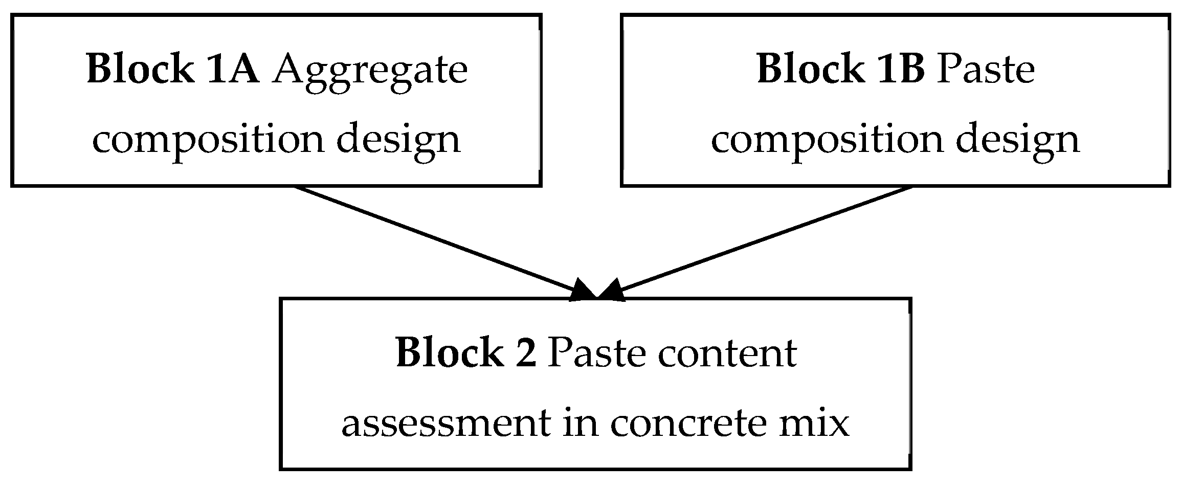
2.5. The Auhor’s Method of SCC Composition Design

2.5.1. The Method Principle

The design method described in Refs. [3,13,14] is based on the very simple scheme shown in Figure 1, where both first level blocks are designed independently. That is why this part of work is organized in the same pattern: aggregate testing and composition design, paste testing and composition design, and concrete mix composition design and testing.

2.5.2. Aggregate Block (1A)

The principle of aggregate composition design is to minimize voids in a loose state of aggregate using successive approximation method. The loose state is chosen to ensure good self-compactibility and low risk of coarse aggregate settlement in formwork. This is based on the assumption that any granular matter has to obtain a loose state during free flow. When the density of this matter during the flow is as high as possible and all voids are properly filled with fluid—but with only small excess (i.e., as low as possible)—after the flow stoppage, the loose state remains “frozen”, guaranteeing good settlement prevention. It was shown in Ref. [13] that typically, the range of similar (i.e., within the error of its estimation) voids content in a loose state is very broad, even up to a 10% sand-to-total-aggregate ratio (s/a). This parameter value is directly proportional to water demand, so it may be used as a secondary criterion for the quick choice of optimum aggregate composition estimation.

2.5.3. Cement Paste Block (1B)

The principle of this design stage is to obtain a ready-to-use cement paste of fluidity high enough to obtain the self-compactibility of concrete but low enough to prevent settlement/sedimentation problems. The fluidity is estimated on Haegerman’s cone slump flow test. The goal is to obtain visible—but not severe—sedimentation after the slump flow stoppage. This is demonstrated in Figure 2 (exemplary photographs, from different testing series). Part (a) shows the example of stable paste. Part (b) presents a “Visible sedimentation” case, i.e., the lightest component of paste (typically addition—here: limestone powder) is easy visible on the “cake” surface. Part (c) reveals a “Severe sedimentation” case, i.e., fluid cement milk is visible on the “cake” rim (here, for better contrast, the example with black unburned coal coming from siliceous fly ash is shown). The obtained gap between these two limits is 4–5 cm wide in terms of final slump flow diameter (D₀). Sedimentation occurs at the similar D₀ if only minimum SP content is reached (sp_min). The example is shown below, Section 4. The excess of fluidity (over primary sedimentation limit) is assumed to wet aggregate surface without obtaining visible segregation on concrete slump flow. If it is too small, concrete consistency is too low. If it is too big, concrete mix tends to sedimentate. Finally, a constant fluidity is chosen 1–2 cm below severe sedimentation occurrence.

Looking from the point of view of concrete stability the best proportion of addition (ad) to cement (c) ratio is the one, when the visible sedimentation is obtained on the highest D₀. Such tests are to be performed, if needed, on high sp (i.e., in a range between 75 to 100% of maximum dose allowed by instruction, sp_max).

Next, a required w/c ratio(s) is/are assumed (due to strength and durability reasons). This allows us to calculate the required ad/c ratio (taking into consideration viscosity and stability classes). For a chosen this way binder (b) proportions the test on pastes to establish primary sp is performed. During the test, sp is kept constant and water content steeply raised until at least a visible sedimentation limit is reached. This allows us to obtain curves in a D₀-w/b space. Preferably, the whole range of sp is tested (i.e., from sp_min to sp_max). The example is shown below, Section 4, (see also examples shown in References. [3,13,14])

The next step is to check the fines content in aggregate (f), as their water demand is typically comparable to the binder one. The author uses a washing method according to EN 933-1.

At the end, primary sp value is assessed. The idea is to add fines f to binder, i.e., to obtain b_cor = c + ad + f and to use b_cor to read sp from the D₀-w/b plot (details: see example in Section 4 below).

2.5.4. Paste Content Assessment in Fresh Concrete Block (2)

The principle of this stage is to put aggregate into the mixer and to prepare ready-to-use cement paste in a separate bucket. Next, the mixer is turned on and the paste is added step-by-step to the mixer until the required consistency level is obtained.

2.6. The Assumptions of the Research Program

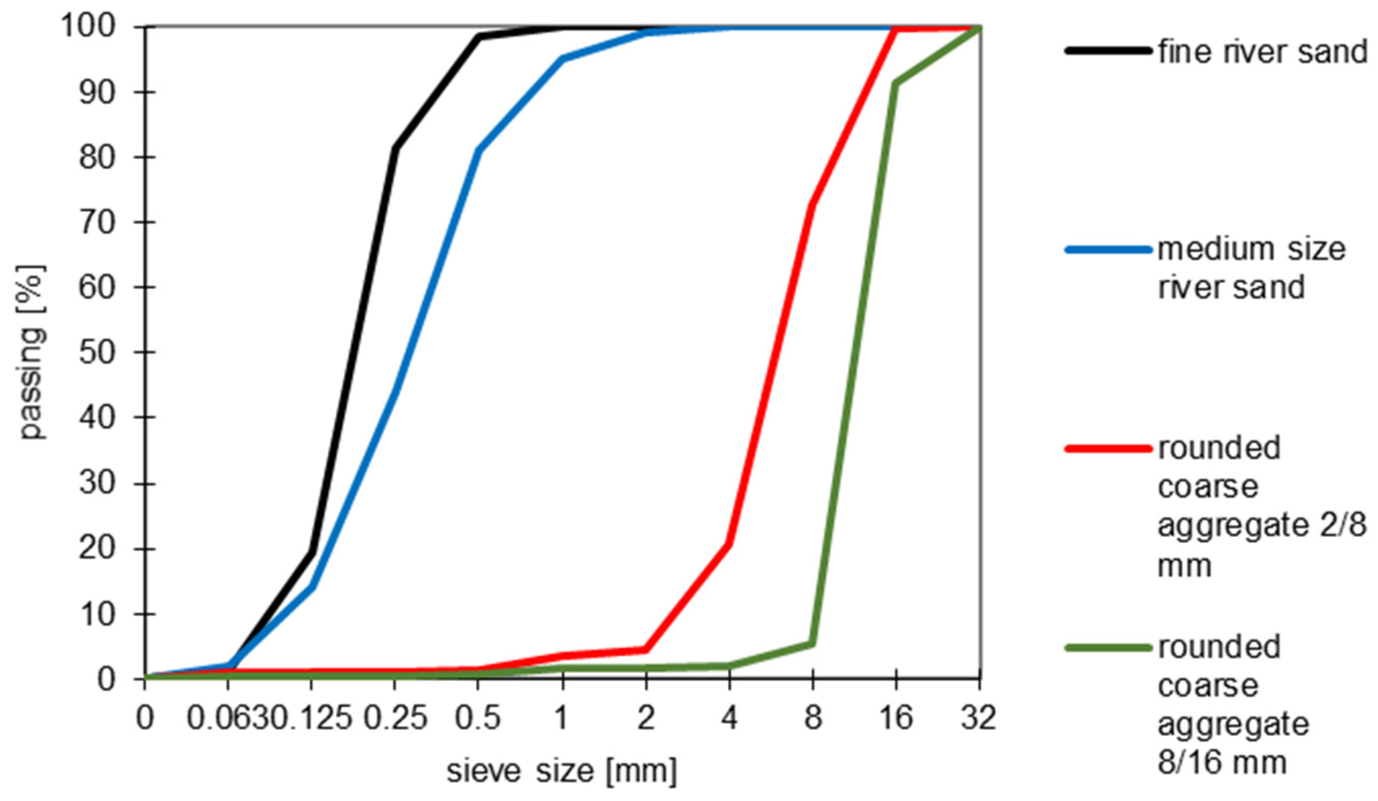
Due to the aim of the research, i.e., to test the usability of the methods for assessing the water demand of aggregates, it was decided to select the widest possible range of aggregate grading compositions in this respect. For this purpose, the same set of 12 compositions which were successfully tested in the previous research program was adopted [13]. Therefore, materials from the same local source were used—of course from new deliveries. The same decision was taken for the components of the paste, but it was decided to optimize the paste not taking into consideration the previous compositions. In order to limit the number of variable parameters, 1 basic level w/b ratio and one level ad/c ratio were adopted. Additionally, for the selected four aggregate compositions, two additional levels of w/b ratio were tested, similarly to the program presented in Ref. [13].

3. Materials

The aggregate was delivered by two local suppliers. The first one delivered fine sand, and the second one delivered the lasting three materials. The parent rock for all of these materials was Carpathian flysch containing mostly sandstone and schist.

Cement paste was composed from commercial CEM II/B-S 32.5R cement (Heidelberg Materials, Poland), commercial limestone powder dedicated to SCC (Lafarge, Poland) and a polycarboxylate type superplasticizer (Sika, Poland).

4. Research Program and Main Results

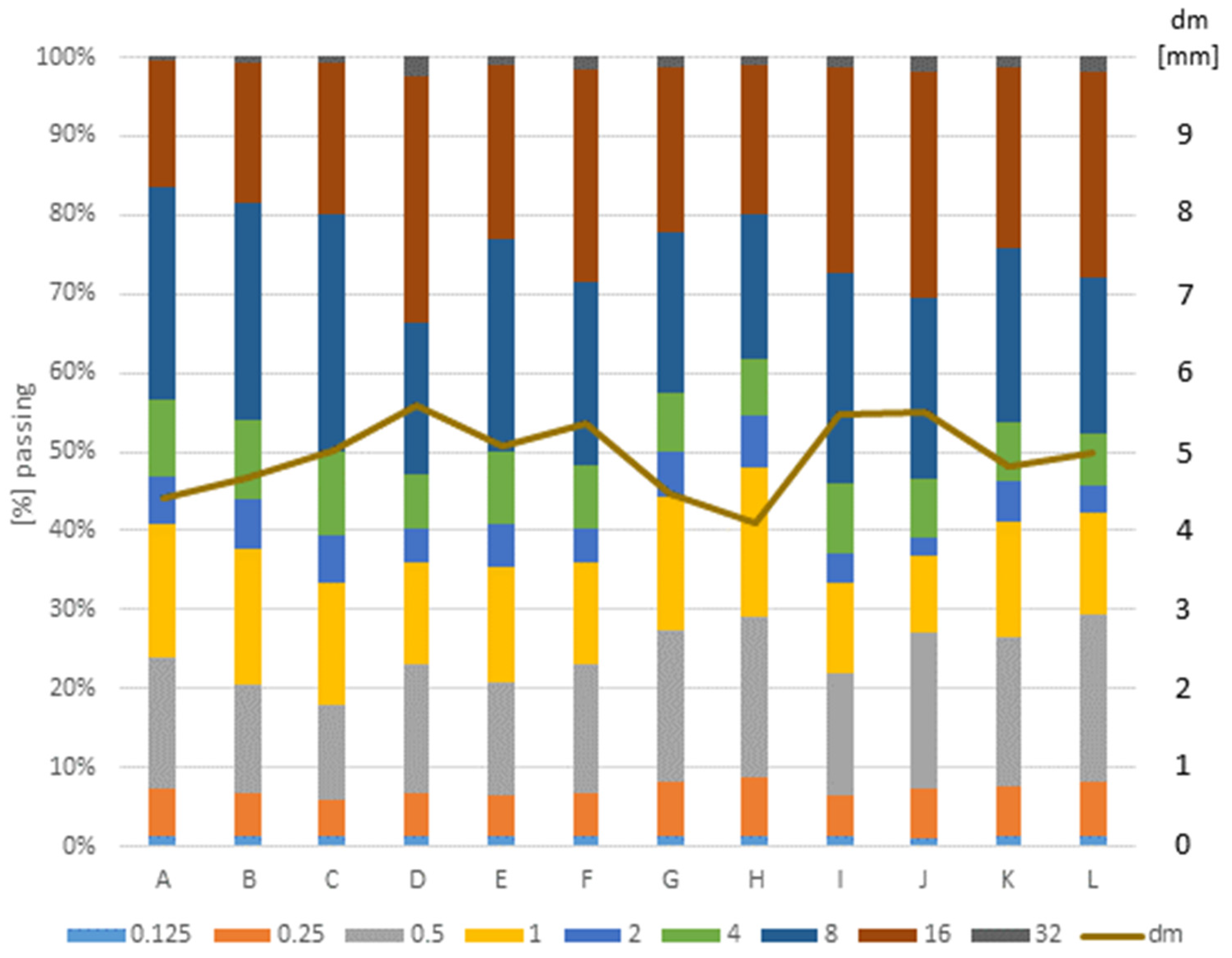
4.1. Aggregate Block (1A)

Aggregate grading curves differed only very slightly from those described in Ref. [13] (max. 5%, average 2% in particle distribution curve of component aggregates). The particle distribution curves of the component aggregates used are shown in Figure 3. As the 2/8 mm fraction coarse aggregate contained a significant oversize (25%), it had to be compensated by the reduced dose of 8/16 mm size aggregate. The difference in the s/a ratio (i.e., the percentage content of grains up to 2 mm in the entire aggregate mass) compared to the value from [13] was approximately +1%. The grading curves were therefore comparable to the previous ones. The loose state density difference between both series was within the measurement error (the error calculation was described in Ref. [13]).

The grading curves of obtained compositions (in mass units, i.e., as for calculations using the Stern, Bolomey, and RSS methods) are shown in Figure 4. Fine content in aggregate was tested using the washing method according to EN 933-1 [38]. The aggregate compositions are denoted by capital letters A–L, as shown on the horizontal axis.

4.2. Cement Paste Block (1B)

The stability check (ad/c value assessment) results are given in

Table 1. Addition dosage assessment (sp = 0.75 sp_max).

Parameter	Value
ad/c	0	0.1	0.2	0.3	0.4	0.5	0.6
D0 stab [cm]	34	36	37	38	38	38	37

. D_{0 stab} is a slump flow diameter of Haegermann’s cone when the first traces of paste instability on the “cake” surface are detected.

So that stability criterion was chosen at ad/c = 0.3 and fluidity one at D₀ = 39 cm. This value is presented in Figure 5 as a vertical, black dotted line. w/b ratios were kept at the same levels like in Ref. [13], it means that the main level was set at 0.4, and the supplementary ones at 0.34 and 0.46.

Since the measured content of fines in the aggregate f was within a quite narrow range of 2–2.6% (see Figure 3), a constant value equal to the average one (2.4%) was set for the calculations. Another needed assumption was the paste content equal to the average value from the program [13] equal to 350 dm³/m³. This means that f = 22.25 kg/m³ of surplus powders was added with the aggregate.

However, after performing a test mix on the concrete scale, it turned out that the paste lost fluidity in the mix much more than in the previous program. Since the aggregate in both cases was very similar (mineral and grain composition, fines content), it can be hypothesized that the SP also adhered to the aggregate grains, not only to the powders. In order to limit the number of variables in the research program, it was decided to omit this problem by adopting the value of b_cor = c + ad + 2f for better compensation of consistency loss. The test results are shown in Figure 5. The minimum sp value to obtain required paste fluidity is 0.4% of binder/powder mass, for w/b_cor ≈ 0,41. In the opposite edge, the maximum reasonable sp is between 1.2 and 1.6%, for w/b_cor ≈ 0.2. Within this last range, the accuracy of sp prediction is low, below 1.2%—good. In this way, the sp values presented in

Table 2. Superplasticizer dosage assessment.

Parameter	Paste
w/b	0.34	0.40	0.46
w/bkor	0.313	0.365	0.417
sp [% b]	0.67	0.5	0.4

were obtained. In the case of a non-exact match, linear interpolation was used.

4.3. Fresh Concrete Block (2)

The fresh concrete block part of the research program was performed following the abovementioned procedure (Section 2.5.4), as follows. Test mixes with a volume of approximately 15 dm³ were assumed. Firstly, the cement paste was prepared in a bucket using an appropriate size submersible mortar mixer. Typically, ca. 60–70 s mixing procedure was used, pouring powders to the liquid within 5–7 s. The paste volume was designed in excess, assuming that its consumption would be approximately 430 dm³/m³. Secondly, the aggregate was placed in a laboratory counter-current mixer with a maximum capacity of 25 dm³, and the ready-mixed paste was gradually poured during mixing until the target consistency was achieved. Typically, ca. 30 s interval between pours was used. When consistency seemed to be visually satisfactory, final mixing for ca. 120 s was performed. At the first attempt, the target consistency was set around the self-compaction limit in the sense of European requirements (i.e., EN 206 [42]). This means that the target values were D₀ = 550 ± 20 mm and t_V = 25 ± 3 s. After mixing, consistency tests were performed (Abrams cone flow D₀, t₅₀₀ time, t_V time; all according to EN 12350 [43,44]). The tests were performed within 5–6 min. Next, the mix was placed back in the mixer and another (single) portion of the paste was added, corresponding to an increase in its content in 15–30 dm³/m³ (i.e., aiming to obtain the next consistency level) of concrete, and the 120–150 s mixing time was applied. This way, 2–3 consistency measurements were obtained from one batch. Then, the second batch of the same composition was prepared in the same way. The first measurement was made at the paste content estimated on the basis of the results of the first batch as the “exact” self-compacting limit. The second measurement from this batch was to reflect one of the measurements from the first batch to compare the results (with an accuracy of 3 dm³/m³ due to weight tolerance and the fact that some minimal losses of paste during testing are unavoidable). Sometimes a third measurement was also performed to obtain a wider range of tested consistencies.

The obtained concrete compositions are presented in Figure 6 and in Appendix A. Notations of SCC mixes are presented on the horizontal axis. The number denotes assumed w/b ratio, and a capital letter following this number—the notation of aggregate composition, following Figure 4. Consistency level denoted “0” means borderline consistency as defined above. The “+1” consistency level denotes the first obtained consistency level above the limit, “−1”—the first one below the limit, and so on.

The results of consistency measurements are summarized in Figure 6, Figure 7 and Figure 8. The repeated compositions were either “1” or “0” ones. “0” composition was repeated when the exact self-compactibility limit was obtained on the first batch; otherwise, composition “1” was repeated. The maximum difference between repeated compositions was ±35 mm for D₀, ±2.5 s for t₅₀₀, and ±2 s for t_V. In these cases, average values were used to plot the points in Figure 6, Figure 7, Figure 8 and Figure 9. For a “40 L” composition, an example without averaging is shown (consistencies “−1” and “0”): ΔV_p = 2 dm³, ΔD₀ = 3 cm, Δt₅₀₀ = 1,9 s, t_V—without comparison, because it was initially assumed that if t₅₀₀ > 12 s was obtained, t_V testing was omitted due to the expected testing time being too long (which turned out to be an error in this particular case).

5. Discussion

Figure 10 and Figure 11 present the results of the analyses of models (15)–(18). To make the comparison between models easier, the calculations were made assuming the constants χ_i = 1. The model based on the Bolomey formula is presented in a separate figure due to the different magnitude of the obtained values.

A very high level of fit was achieved in all cases (R² between 0.95 and 0.985). This means that all four presented models are verified positively and that there is no need to work on the new model. It also means that the water demand/specific surface area of the aggregate can certainly be treated as the dominant parameter that determines the cement paste content necessary to achieve self-compactibility limit of SCC. That is why this line may be called the “minimum paste demand line”. Additionally, there is a clear indication that non-linear models (i.e., by Stern and Bolomey) are more precise (98% of good fit vs. 95.2% for the linear ones).

Next, the constants of all models were calibrated so as to obtain the same t_rel at the point of the average value of V_p = 350.5 dm³/m³. χ_O = 1.55 was assumed as a reference point. The results of this calibration are shown in Figure 12. Noteworthy here is a slightly different angle of inclination of the line obtained for the ONT model. The special feature of this model is the use of volume units to determine ∑_a. It can be hypothesized that this is related to the lack of the factor φ_a in the denominator of the expression in the t_relO model (15), but confirming this hypothesis would require the use of additional models using volume units.

Table 3. Comparison between χ_i parameter values depending on the “base” χ_O value and their influence on the final t_rel value.

Shape of Grains/ Aggregate Type	χO	χR	χS	χB	trel (Vp = 350)
Ideal spheres	1.66	1.07	0.38	65.80	0.0561
Rounded grains (river origin)	1.55	1.00	0.355	61.45	0.0524
Coarse aggregate partly crushed (grit) + river sand	1.50	0.97	0.34	59.45	0.0507
Crushed coarse aggregate + river sand	1.43	0.92	0.325	56.70	0.0484
Only crushed grains	1.33	0.86	0.305	52.725	0.0449

lists the χ_i parameter values depending on the adopted reference value χ_O. The match between the χ_i values and the type of aggregate used should be treated as a rough indication, as even small changes in V_p alter the obtained χ_i values significantly.

Additionally, the table shows the difference in t_rel value in these cases. The difference between the cases of ideal spheres and crushed aggregate is 24.4%, so it is a very important one. The replacement of rounded river origin coarse aggregate by the crushed one is smaller, but still significant (8.5%). Only the difference between rounded coarse aggregate and a grit is acceptable (ca. 3.5%). This means that the comparability of the t_rel determination results between different sets of aggregates of the same type should be considered limited but not excluded, contrary to comparison between different types of aggregate, which is highly questionable.

Theoretically, it is possible to determine the value of χ_O using Equation (11) directly, i.e., putting the real values of V_exc calculated by definition as a difference between V_p and a loose packing density of aggregate. Unfortunately, this method is highly questionable, as it has a very high risk of obtaining a very large dispersion of results. Each change—even a very small one in the paste content (V_p), which does not affect the measured consistency (e.g., 3 dm³/m³)—significantly shifts the paste demand line along both axes. The coefficient χ_i, on the contrary, influences the t_rel axis only. This is demonstrated in Figure 13 by the “one composition” line; a change in D₀ by 5 cm was achieved at ΔV_p from the range of around 15–20 dm³.

Figure 13, Figure 14 and Figure 15 present the three basic SCC consistency measures influence on the t_rel values, using the example of ONT model (15), assuming χ_O = 1. The correlation is always linear, and the lines are more or less parallel. The deviations from the parallel pattern and low fit (low R²) are most probably caused by the lower precision of the obtained results. In these cases the research program was not designed to minimize the error in the same way like in the case of the results shown in Figure 10 and Figure 11. Moreover, the range of values taken into account as one series in the case of Figure 13, Figure 14 and Figure 15 is wider. This resulted in some cases in more than one data point covered by a given consistency range, see example in Figure 14. Each such case significantly increases the standard deviation value and reduces the resulting R² value. This may significantly affect the final angle of inclination of the obtained regression line.

In summary, the presented method allows determination of the paste demand line for any SCC consistency test in scope (slump flow and viscosity measures) at any selected limit value. It should be noted that in the described method, it is not possible to estimate the content of cement paste necessary to increase consistency using an integrated consistency factor (like in the case of traditional water demand assessment methods). Here, this is performed by parallel shifting of the paste demand line along the line of increasing paste content, as shown in Figure 13 and Figure 14; the line is shifted along both axes, not along the t_rel axis solo.

The SCC composition design method using proposed minimum paste demand line may be summarized as follows [19].

• Design 4 mixes of extreme compositions in terms of t_rel using the method proposed in Section 2.5.2 and Section 2.5.3. This means that 2 extreme values of both w/b ratios (for extreme ∑_p obtaining) and water demand/specific surface of aggregate (for extreme ∑_a obtaining) are to be selected. As a quick indicator of the second value, a sand (i.e., aggregate up to 2 mm)-to-total aggregate ratio (s/a) may be used.
• Test the designed mixes according to Section 2.5.4. The target is to obtain the assumed consistency level.
• Calculate t_rel values for the designed concrete compositions and plot linear regression curve in the V_p − t_rel space to obtain the minimum paste demand line.
• Design composition conforming to a pre-assumed specification (e.g., strength class, etc.) of t_rel within the range covered by the line and read predicted V_p for this case.
• Prepare the trial batch using predicted V_p and adjust (rise) sp if necessary.

In the present version, the proposed approach enables to predict paste volume for SCC assuming a given aggregate and paste compositions. Unfortunately, it underestimates the superplasticizer dose (sp). The procedure of cement paste assessment described in Section 2.5.3 sets a bottom limit for sp, not a target value. Obtaining a more reliable sp will be the next step of the presented approach development. The examples of the proposed approach implementation are shown in details in Ref. [14].

6. Conclusions

The presented results and their analysis allow the following general conclusions to be formulated:

• The water demand/specific surface area of aggregate is a key factor determining the content of cement paste necessary to achieve self-compaction ability of concrete.
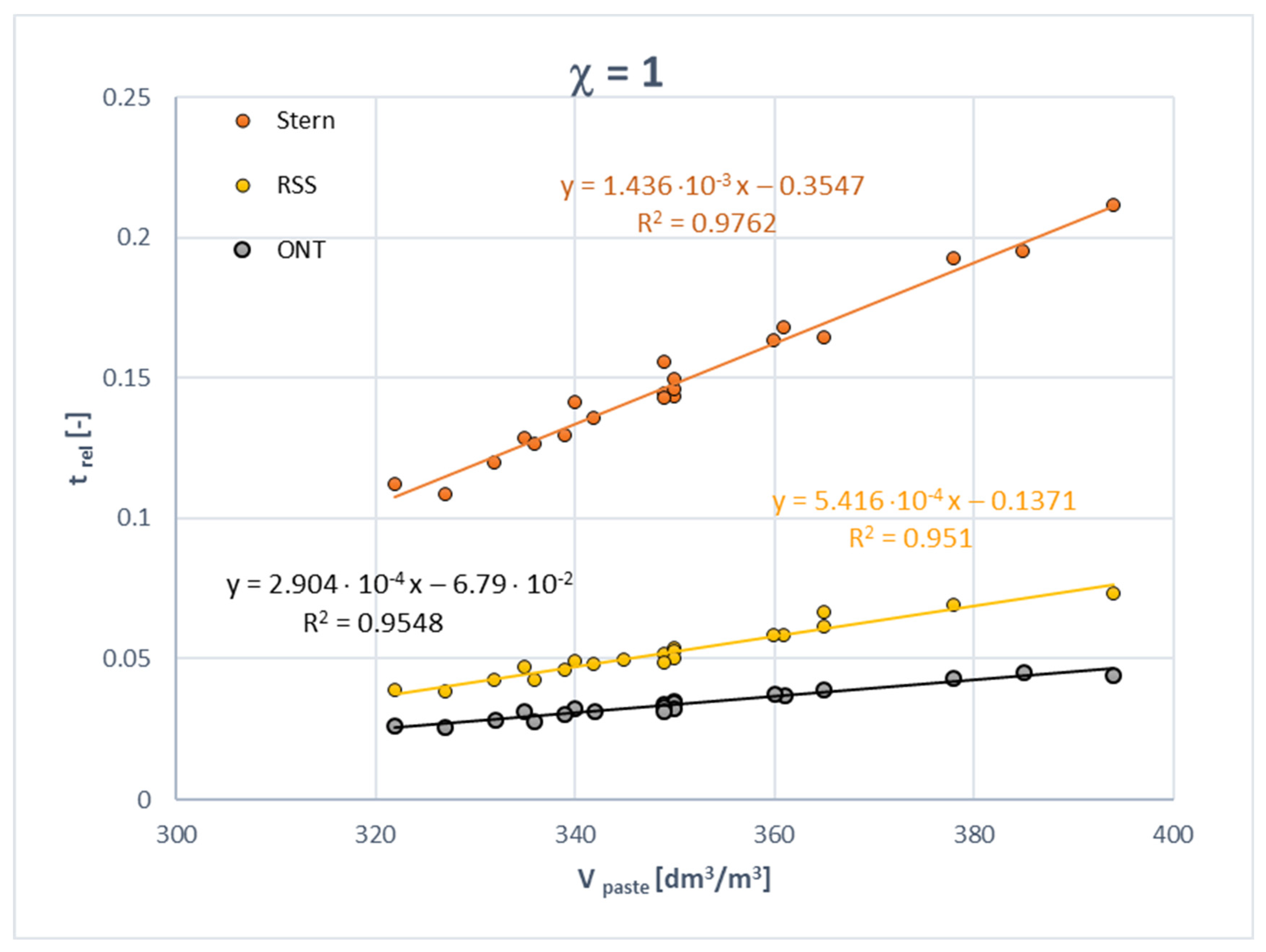
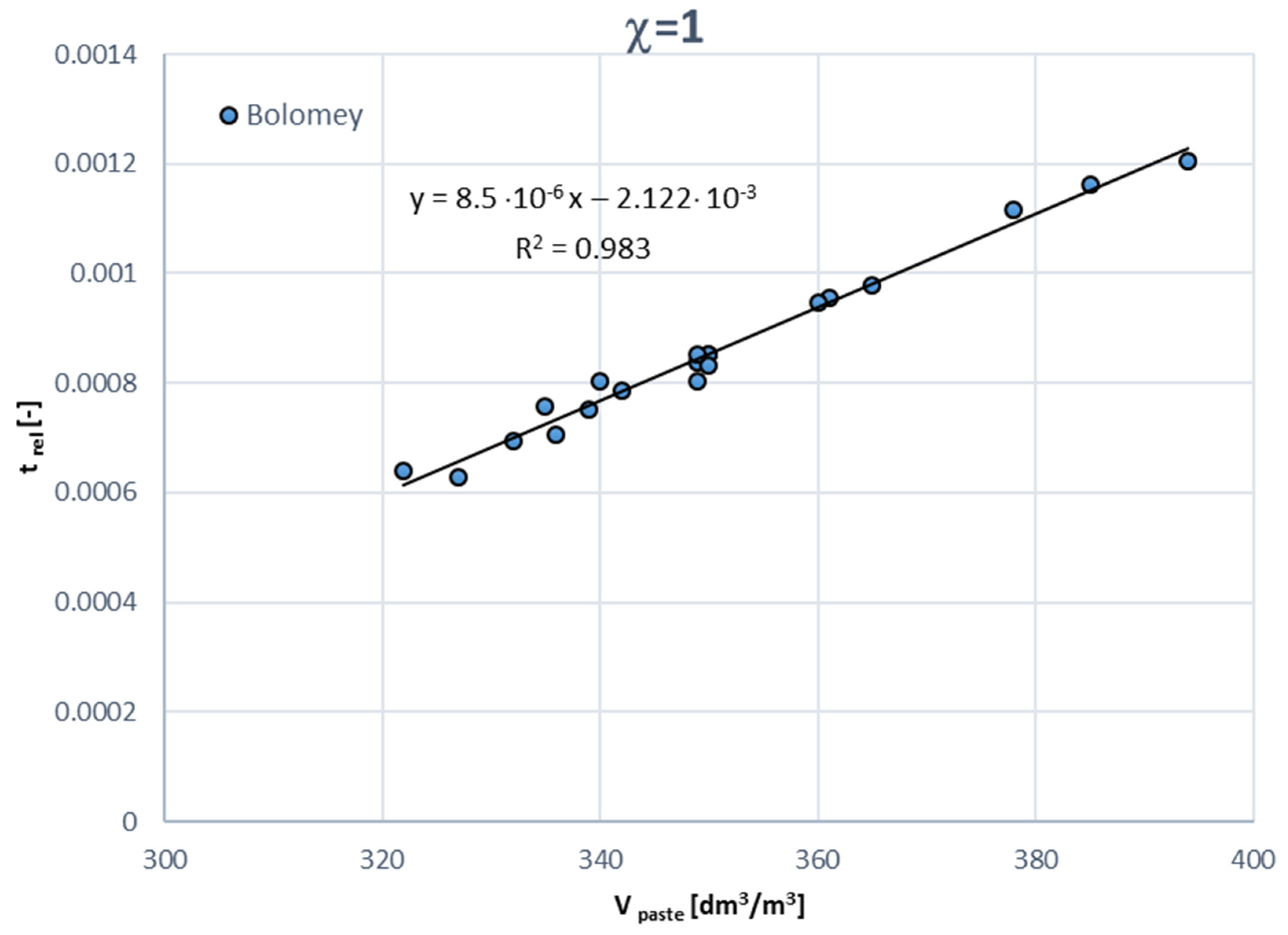
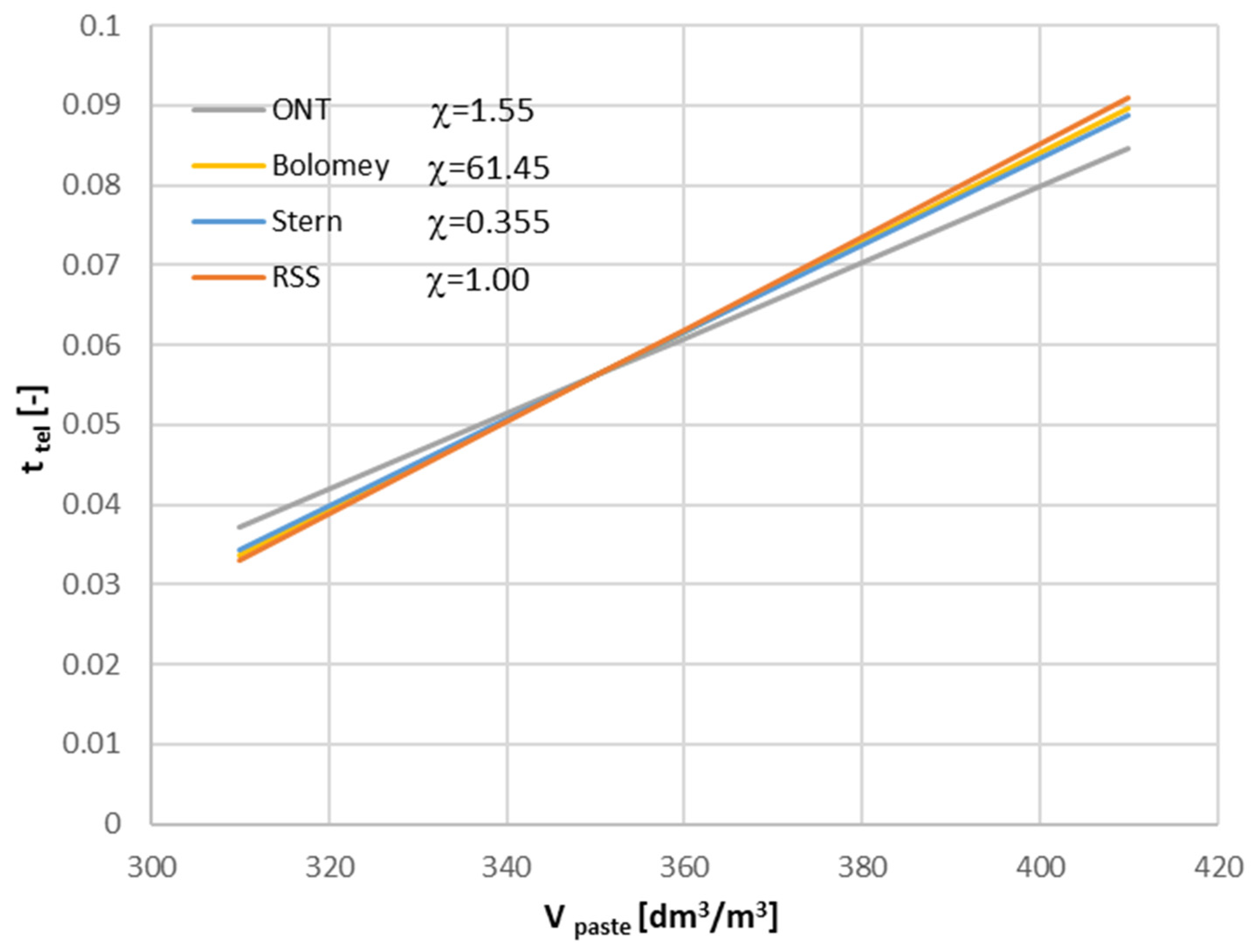
• The traditional methods of water demand/specific surface of aggregate assessment (Stern, Bolomey/Loudon based, RSS) are also valid in the SCC case and they may be used without any alteration. The best fit was obtained for traditional non-linear water demand models (by Stern and by Bolomey).
• The presented method allows to predict paste volume of SCC basing on specific surface/water demand of aggregate and the simple procedure to obtain cement paste of the proper fluidity. The capability to allow prediction of superplasticizer dosage needs further work.
• The method allows to assess minimum paste demand for any specified range for slump flow, t₅₀₀, and V-funnel tests.
• The disadvantage of the described approach is the need to use an arbitrarily determined integrated coefficient containing the total effect of grain shape, unit conversion, model constants, etc. Therefore:
  • The applicability of the model should be limited to a fixed set of component aggregates used to compose the aggregate skeleton.
  • The comparability of results between compositions containing aggregate of the same type (e.g., rounded) but of different origin should be considered limited.
  • The comparability of results between types of aggregates (rounded/crushed) should be considered questionable.

References

1. Ashisch, D.K.; Verma, S.K. An overview on mixture design of SCC. Struct. Concr. 2019, 20, 371–395. [Google Scholar] [CrossRef]
2. De Schutter, G.; Gibbs, J.; Domone, P.; Bartos, P.J.M. Self-Compacting Concrete; Whittles Publishing: Scotland, UK, 2008; ISBN 978-1904445-30-2. [Google Scholar]
3. Urban, M. The new conception of SCC composition design: Theoretical background, evaluation, presentation of procedure and examples of usage. Mater. Struct. 2015, 48, 1321–1341. [Google Scholar] [CrossRef]
4. Shi, C.; Wu, Z.; Lv, K.X.; Wu, L. A review on mixture design methods for SCC. Constr. Build. Mat. 2015, 84, 387–398. [Google Scholar] [CrossRef]
5. Kohler, E.P.; Fowler, D.W.; Foley, E.H.; Rogers, G.J.; Watanachet, S.; Jung, M.J. SCC for Precast Structural Applications: Mixture Proportions, Workability, and Early-Age Hardened Properties. CTR Technical Report; The University of Texas at Austin: Austin, TX, USA, 2008; pp. 51–66. [Google Scholar]
6. Trejo, D.; Hendrix, G. Influence of Aggregate and Proportions on Flowing Concrete Characteristics. ACI Mater. J. 2018, 115, 171–180. [Google Scholar] [CrossRef]
7. Zuo, W.; Liu, J.; Tian, Q.; Xu, W.; She, W.; Feng, P.; Miao, C. Optimum design of low-binder SCC based on particle packing theories. Constr. Build. Mater. 2018, 163, 938–948. [Google Scholar] [CrossRef]
8. Sebaibi, N.; Benzerzour, M.; Sebaibi, Y.; Abriak, N.-E. Composition of SCC using the CPM, the Chinese method and the European standard. Constr. Build. Mater. 2013, 43, 382–388. [Google Scholar] [CrossRef]
9. Brouwers, H.J.H.; Radix, H.J. SCC: Theoretical and experimental study. Cem. Concr. Res. 2005, 35, 2116–2136. [Google Scholar] [CrossRef]
10. Li, P.; Ran, J.; Nie, D.; Zhang, W. Improvement of mix design method based on paste rheological threshold theory for SCC using different mineral additions in ternary blends of powders. Constr. Build. Mater. 2021, 276, 122194. [Google Scholar] [CrossRef]
11. Kheder, G.F.; Al Jadri, R.S. New method for proportioning SCC based on compressive strength requirements. ACI Mater. J. 2010, 107, 490–497. [Google Scholar]
12. Kuczyński, W. (Ed.) Budownictwo Betonowe, t. 1 Technologia betonu, cz. 2. Projektowanie betonów. In Concrete Engineering, Part 1 Technology of Concrete; Arkady: Warszawa, Poland, 1972. (In Polish) [Google Scholar]
13. Urban, M. Zawartość zaczynu jako główne kryterium projektowania BSZ. (Paste content as a main criterion for SCC composition design). Mater. Bud. 2017, 540, 83–86. [Google Scholar]
14. Urban, M. Two limiting lines technique to obtain minimum paste demand of self-consolidating concrete. ACI Mater. J. 2019, 116, 131–138. [Google Scholar] [CrossRef]
15. Oh, S.G.; Noguchi, T.; Tomosawa, F. Toward mix design for rheology of SCC. In Proceedings of the PRO 007: 1st International RILEM Symposium, Stockholm, Sweden, 13 September 1999; pp. 361–372. [Google Scholar]
16. Marquardt, I.; Vala, J.; Diederichs, U. Optimization of SCC mixes. In Proceedings of the 2nd International Symposium on SCC, Tokyo, Japan, 23–25 October 2001; pp. 295–302. [Google Scholar]
17. Xie, Y.; Liu, Y.; Long, G. A mix design method for SCC. In Proceedings of the PRO 054: 5th International RILEM Symposium on Self-Compacting Concrete, Ghent, Belgium, 3–5 September 2007; pp. 189–198. [Google Scholar]
18. Su, N.; Hsu, K.-H.; Chai, H.-W. A simple mix design method for SCC. Cem. Concr. Res. 2001, 31, 1799–1807. [Google Scholar] [CrossRef]
19. Liu, L.; Lei, M.; Gong, C.; Gan, S.; Yang, Z.; Kang, L.; Jia, C. A robust mix design method for SCC. Constr. Build. Mater. 2022, 352, 128927. [Google Scholar] [CrossRef]
20. Sedran, T.; de Larrard, F. Optimization of self-compacting concrete thanks to packing model. In Proceedings of the PRO 007: 1st International RILEM Symposium, Stockholm, Sweden, 13 September 1999; pp. 321–332. [Google Scholar]
21. Okamura, H.; Ozawa, K. Mix design method for SCC. Concr. Libr. JSCE 1995, 25, 107–120. [Google Scholar]
22. Van, B.K.; Montgomery, D. Mixture proportioning method for SCC HPC with minimum paste volume. In Proceedings of the PRO 007: 1st International RILEM Symposium, Stockholm, Sweden, 13 September 1999; pp. 373–384. [Google Scholar]
23. Alyamac, E.; Ince, R. A preliminary concrete mix design for SCC with marble powders. Constr. Build. Mater. 2009, 29, 1201–1210. [Google Scholar] [CrossRef]
24. Wang, Z.; Wu, B. Mix design method for self-compacting recycled aggregate concrete targeting slump-flow and compressive strength. Constr. Build. Mater. 2023, 404, 133309. [Google Scholar] [CrossRef]
25. Nataraja, M.C.; Gadkar, A.; Jogin, G. A simple mix proportioning method to produce SCC based on compressive strength requirement by modification to IS 10262:2009. Indian Concr. J. 2018, 92, 15–23. [Google Scholar]
26. Jamroży, Z. Beton i jego technologie. In Concrete and Its Technologies; PWN: Warszawa/Kraków, Poland, 2006; ISBN 83-01-13253-1. (In Polish) [Google Scholar]
27. Piasta, J.; Piasta, W.G. Beton zwykły. In Ordinary Concrete; Arkady: Warszawa, Poland, 1994; ISBN 83-213-3667-1. (In Polish) [Google Scholar]
28. Śliwiński, J. Beton zwykły–projektowanie i podstawowe właściwości. In Ordinary Concrete–Design and Basic Properties; Polski Cement: Kraków, Poland, 1999; ISBN 83-907640-3-2. (In Polish) [Google Scholar]
29. Wang, Q.; Jingjang, H.; Sun, J.; Ho, J. Determining the specific surface area of coarse aggregate based on sieving curve via image-analysis approach. Constr. Build. Mater. 2021, 305, 124728. [Google Scholar] [CrossRef]
30. Cepuritis, R.; Garboczi, E.J.; Ferraris, C.F.; Jacobsen, S.; Sorensen, B.E. Measurement of particle size distribution and specific surface area for crushed concrete aggregate fines. Adv. Powder Technol. 2017, 28, 706–720. [Google Scholar]
31. Maroof, M.A.; Mahboubi, A.; Noorzad, A. A new method to determine specific surface area and shape coefficient of a cohesionless granular medium. Adv. Powder Technol. 2020, 31, 3038–3049. [Google Scholar] [CrossRef]
32. Wong, H.H.C.; Kwan, A.K.H. Packing density of cementitious materials: Part 1—Measurement using a wet packing method. Mater. Struct. 2008, 41, 689–701. [Google Scholar] [CrossRef]
33. Kwan, A.K.H.; Li, L.G. Combined effects of water film, paste film and mortar film thicknesses on fresh properties of concrete. Constr. Build. Mater. 2014, 50, 598–608. [Google Scholar] [CrossRef]
34. Bucher, R.; Diederich, P.; Mouret, M.; Escadeillas, G.; Cyr, M. SCC using flash-metakaolin: Design method. Mater. Struct. 2015, 48, 1717–1737. [Google Scholar] [CrossRef]
35. Barrioulet, M.; Legrand, C. Influence of the interstitial paste on the flow ability of fresh concrete. The importance of water retained by the aggregates. Mater. Struct. 1977, 10, 365–373. [Google Scholar]
36. Bolomey, J. Module de Finese d’Abrams et Calcul de L’eau de Gachage des Betons; EMPA: Zurich, Switzerland, 1930. [Google Scholar]
37. Stern, O. Zielsiechere Betonbildung; Springer Verlag: Berlin, Germany, 1934. [Google Scholar]
38. EN 933-1:2012; Test for Geometrical Properties of Aggregate—Part 1: Determination of Particle Size Distribution—Sieving Method. British Standards Institution: London, UK, 2012.
39. Westerholm, M.; Lagerblad, B.; Silfwerbrand, J.; Forssberg, E. Influence of fine aggregate characteristics on the rheological properties of mortars. Cem. Concr. Compos. 2008, 30, 274–282. [Google Scholar] [CrossRef]
40. Bengtsson, M.; Evertsson, C.M. Measuring characteristics of aggregate material from vertical shaft impact crushers. Miner. Eng. 2006, 19, 1479–1486. [Google Scholar] [CrossRef]
41. De Schutter, G.; Poppe, A.-M. Quantification of the water demand of sand in mortar. Constr. Build. Mater. 2004, 18, 517–521. [Google Scholar] [CrossRef]
42. EN 206:2013; Concrete—Specification, Performance, Production and Conformity. British Standards Institution: London, UK, 2013.
43. EN 12350 -8: 2019; Testing Fresh Concrete—Part 8: Self-Compacting Concrete—Slump-Flow Test. British Standards Institution: London, UK, 2019.
44. EN 12350 -9: 2012; Testing Fresh Concrete—Part 9: Self-Compacting Concrete—V-Funnel Test. British Standards Institution: London, UK, 2012.
Figure 1. The block diagram of used SCC design method described in detail in Refs. [3,19,20].
Applsci 14 11108 g001
Figure 2. Sedimentation of the cement paste tested using Haegerman’s cone—exemplary photographs. (a) No sedimentation, (b) visible sedimentation (acceptable/target), (c) severe sedimentation (unacceptable).
Applsci 14 11108 g002
Figure 3. Particle size distribution curves of the component aggregates used.
Applsci 14 11108 g003
Figure 4. Particle size distribution and dm values for aggregate compositions used in the research program.
Applsci 14 11108 g004
Figure 5. Cement paste testing phase. The selection of the superplasticizer content.
Applsci 14 11108 g005
Figure 6. Cement paste contents (Vp) used in the tested SCC compositions.
Applsci 14 11108 g006
Figure 7. Abrams cone flow test results (D0).
Applsci 14 11108 g007
Figure 8. t500 test results.
Applsci 14 11108 g008
Figure 9. V-funnel test results (tV).
Applsci 14 11108 g009
Figure 10. The correlation between Vp and trel for ONT (15), Stern (17) and RSS (18) models, assuming χi = 1.
Applsci 14 11108 g010
Figure 11. The correlation between Vzp and trel for the Bolomey (16) model, assuming χi = 1.
Applsci 14 11108 g011
Figure 12. The assessment of χi coefficient.
Applsci 14 11108 g012
Figure 13. The influence of slump flow diameter D0 on the ONT model (15), assuming χO = 1.
Applsci 14 11108 g013
Figure 14. The influence of t500 time on the ONT model (15), assuming χO = 1.
Applsci 14 11108 g014
Figure 15. The influence of V-funnel tV time on the ONT model (15), assuming χO = 1.
Applsci 14 11108 g015