Article

Heart Sound Classification Using Harmonic and Percussive Spectral Features from Phonocardiograms with a Deep ANN Approach

1
Computer Science and Engineering Department, Thapar Institute of Engineering & Technology, Patiala 147004, India
2
Electrical and Instrumentation Engineering Department, Thapar Institute of Engineering & Technology, Patiala 147004, India
*
Author to whom correspondence should be addressed.
Appl. Sci. 2024, 14(22), 10201; https://doi.org/10.3390/app142210201
Submission received: 30 August 2024 / Revised: 23 October 2024 / Accepted: 27 October 2024 / Published: 6 November 2024
(This article belongs to the Special Issue Machine Learning in Biomedical Applications)

Abstract

:
Cardiovascular diseases (CVDs) are a leading cause of mortality worldwide, with a particularly high burden in India. Non-invasive methods like Phonocardiogram (PCG) analysis capture the acoustic activity of the heart. This holds significant potential for the early detection and diagnosis of heart conditions. However, the complexity and variability of PCG signals pose considerable challenges for accurate classification. Traditional methods of PCG signal analysis, including time-domain, frequency-domain, and time-frequency domain techniques, often fall short in capturing the intricate details necessary for reliable diagnosis. This study introduces an innovative approach that leverages harmonic–percussive source separation (HPSS) to extract distinct harmonic and percussive spectral features from PCG signals. These features are then utilized to train a deep feed-forward artificial neural network (ANN), classifying heart conditions as normal or abnormal. The methodology involves advanced digital signal processing techniques applied to PCG recordings from the PhysioNet 2016 dataset. The feature set comprises 164 attributes, including the Chroma STFT, Chroma CENS, Mel-frequency cepstral coefficients (MFCCs), and statistical features. These are refined using the ROC-AUC feature selection method to ensure optimal performance. The deep feed-forward ANN model was rigorously trained and validated on a balanced dataset. Techniques such as noise reduction and outlier detection were used to improve model training. The proposed model achieved a validation accuracy of 93.40% with sensitivity and specificity rates of 82.40% and 80.60%, respectively. These results underscore the effectiveness of harmonic-based features and the robustness of the ANN in heart sound classification. This research highlights the potential for deploying such models in non-invasive cardiac diagnostics, particularly in resource-constrained settings. It also lays the groundwork for future advancements in cardiac signal analysis.

1. Introduction

In India and across the world, cardiovascular disease (CVD) is a significant cause of death. According to the World Health Organization (WHO) report in 2019 [1], 17.9 million Indians died due to CVD, which contributed to 31.00% of the global deaths from CVD. In total, 85.00% of these deaths were caused by strokes or heart attacks with no prior diagnosis. More than three-quarters of CVD deaths in India happen in lower- or middle-income families, for which affording regular primary healthcare is a significant challenge. Also, another survey from WHO reported that despite the estimated increase in global health professionals to 40 million by 2030, there will still be a shortfall of 18 million by that time [2]. This shortfall is enormous, and particularly in countries with large demographic and geographical diversities like India, it is a big challenge to make such health professionals available on the scale necessary to support CVD-related healthcare for the affected population.
Also, due to the recent COVID-19 pandemic, the number of CVD patients is expected to increase in the coming years [3]. This has motivated the research discussed in this manuscript, where the work related to the intelligent analysis of PCG recordings is presented. This work can further assist healthcare staff in diagnosis and telemedicine services, even in remote locations where only primary healthcare is available. In the past, few computer-assisted decision support systems (DSSs)/expert systems have assisted physicians in minimizing intra- and inter-observer variability. More heart sound data become available has helped practical algorithm developments and supported the cost-effective implementation of artificial intelligence (AI).
Therefore, the use of AI presents an opportunity to address the shortfall problem mentioned in [2] and has been experimentally used by various groups of health organizations to reduce treatment recommendation times with minimal health professional intervention for diseases like diabetes [4], CVD [5], various types of cancers [6], etc. This use of AI minimizes errors and controls disease progression.

1.1. Fundamental Heart Sound

Traditionally, the stethoscope is used to observe heart auscultation. Recognizing pathological heart conditions requires a trained ear. Heart auscultation aims to determine any abnormality in the fundamental heart sound (FHS). A normal FHS consists of two phases, diastole and systole, referred to as the cardiac cycle. Each phase produces a sound based on the opening and closing of heart valves. Thus, in a healthy heart, two sounds occur in a healthy heart, S1 (lub) and S2 (dub), with a rhythm. S1 is produced due to the closing of mitral and tricuspid valves, indicating the start of the systole phase, and S2 is produced due to the closing of aortic and pulmonic valves, indicating the start of the diastole phase. Figure 1, demonstrates the activity of human heart during systole and diastole phase.
Based on the reported research, Table 1 demonstrates the frequency range for various types of heart sounds that a PCG recording may contain.
Several ailments can be indicated through abnormalities in FHS, such as heart arrhythmia, endocarditis, rheumatic heart disease, myocardial infarction, congenital heart disease, etc. [8]. Following heart auscultation, as a follow-up, several tests are carried out to obtain the exact condition of the heart based on invasive and non-invasive procedures. Primarily, ECG is the standard way to recognize early signs of heart abnormalities. However, due to the integration of electronics in the stethoscopes, heart sounds can be recorded as PCG. Moreover, resident doctors can use these recordings or feed into an expert system to support decision-making. The system extracts relevant features from the signal, ultimately helping diagnose [7].

1.2. Standard Procedure for Classifying PCG

The standard approach followed by the reported research includes data acquisition and preprocessing, which is then segmented based on S1 and S2 peaks. Specific localized audio features are extracted, followed by feature selection. These features are then fed to a classification procedure to label the artifacts as normal or abnormal heart sounds or specifically identified ailments [5].These four stages are visually demonstrated in Figure 2. In the literature, among the various procedures, neural network-based classification procedures have outperformed various classic procedures such as SVM, Adaboost, etc. Various neural network architectures have been proposed, and each of these variations considers one or more parameters to introduce improvements to the basic ANN. Neural network-based algorithms, which learn incrementally based on the supervised, unsupervised, or reinforcement learning approach, can be scaled to add more connections without additional maintenance. Their intrinsic design efficiently executes the model over a massive parallel platform and performs massive calculations within the target time range [6]. In most cases, the training and test/validation datasets used are different. If the dataset is too small, the jack-knife technique [9,10] is used.
The key contribution of this research includes the following:
  • The selection of a balanced, usable dataset helps to avoid overfitting and improves the training of the ANN model.
  • Denoising the heart sounds using DWT for signals clipped up to 600 Hz.
  • When harmonic and percussive components are separated in PCG audio analysis, more accurate diagnoses are possible. Harmonic elements uncover periodic structures that are indicative of cardiac conditions. In contrast, percussive elements record important non-periodic events such as murmurs or valve closures, greatly enhancing the assessment of cardiac health assessment.
  • Outliers for each extracted harmonic and percussive feature are determined separately for both labels (i.e., normal and abnormal). This is performed to improve the model training and reduce overfitting.

2. Related Literature

Since 1994, significant research has been published that discusses approaches to simple classifications and identifying specific structural and functional abnormalities of the heart. The research literature published before 2016 was based on data collected from a small group of Outpatient Department (OPD) patients from specific hospitals. However, in 2016, a PhysioNet dataset [11] was published to the research community as a challenge to produce viable AI systems. This dataset is a repository of the best available PCG data of that time. Since then, this dataset has become a benchmark and is used in various research studies discussed further in the proposed methodology.
The reported research is based on heart sound recordings obtained through various types of stethoscopes. The heart sounds are collected from any of four locations: the aortic area (right second intercostal space), pulmonic area (left second intercostal space), tricuspid area (left fourth intercostal space), and mitral area (left fifth intercostal space). While the heart sounds were being recorded, the environmental noise was also being recorded. To reduce such additional noise, various preprocessing techniques were used. Additionally, with few exceptions, the authors generated synthetic dataset samples by intentionally adding noise to the heart sound recording to measure the sensitivity of their presented solution. Moreover, during the investigation of the research literature, it was observed that various neural networks are been trained and tested with or without modification for the classification of FHS. Furthermore, recent research has emphasized the significance of anomaly detection in heart rate data. Staffini et al. [12], Minic et al. [13], and Li et al. [14] highlighted the application of machine learning techniques for anomaly detection in heart rate using ECG. These methods can be extended to enhance the detection of irregular patterns in PCG signals.
Table 2 summarizes the various types of neural networks that were reviewed in the scholarly work under investigation.
Neural networks were trained using backpropagation [27,33,34,35,36,37], with computational complexity and resource and time constraints influencing the choice of network architecture. Moreover, transfer learning [38] enables neural networks to extend knowledge from one domain to a related domain. However, when there is a substantial difference between the pre-trained model’s dataset and the target dataset, it can lead to the transfer of irrelevant or uninformative features. Additionally, challenges such as insufficient fine-tuning data, architectural mismatches, and negative transfer may result in suboptimal performance or outcomes worse than a model trained from scratch.
In addition to neural network approaches, other methods such as CNNs [39], XGBoost decision tree algorithms [40], K-Nearest Neighbors (KNN), Fuzzy K-Nearest Neighbors (Fuzzy KNN) [41], Bayes Net, Naïve Bayes, SGD, and LogitBoost [42] have also been reported in research. These reported algorithms have certain limitations when compared to artificial neural networks (ANNs). In this study, a feed-forward artificial neural network (ANN) was selected over the referenced machine learning models, such as XGBoost, K-Nearest Neighbors, Naïve Bayes, and decision-tree-based methods, due to the specific challenges posed by PCG signal classification. Although models like decision trees and KNN are effective for structured and low-dimensional data, they often struggle to accurately process high-dimensional and non-linear data such as PCG signals, where the relationships between features are complex and interdependent [40].
With its layered architecture, an ANN captures these detailed patterns more effectively based on its ability to introduce non-linearity through activation functions and process multiple layers of features simultaneously. This makes the ANN highly robust against the noise and variability inherent in PCG data, resulting in a more reliable classification performance. Additionally, the ANN offers significant computational advantages, making it suitable for real-time applications. When supported by an appropriate hardware device, its parallel processing capabilities and scalability are critical for deploying PCG classification models in clinical settings, where rapid and efficient data processing is essential. This approach will further emphasize the deep learning model’s strengths and the added value that an ANN brings to PCG signal analysis.

3. Methodology

The steps considered for classifying PCG sound signals as normal or abnormal in the underlying research are highlighted in Figure 3. The PCG sound signals were sourced from the PhysioNet 2016 dataset [11], and based on the analysis provided in the research literature, the dataset was filtered to remove the unusable audio files. The overall research approach for this expert system is divided into four steps: selecting and denoising the data, extracting features from the data, selecting data for training and testing the feed-forward ANN model, and finally, feeding the data to the ANN model to classify the patient condition.

3.1. Dataset Acquisition

Physionet, also known as “Research Resources for Complex Physiologic Signals”, is a repository of extensive clinical and physiological data samples. The dataset, published under the Physionet CINC challenge 2016, contains PCG recordings ranging from 5 to 100 s, recorded under clinical or non-clinical conditions [43]. The dataset is a collection of eight independent heart sound recording datasets referenced in previous research and collected through various clinical and non-clinical settings. For simplicity, all the individual datasets are labeled ‘a’ through ‘i’ [11].
The PCG data sample recordings available in the challenge were collected from 1072 patients, along with information on their heart conditions. More than one recording sample is available from a single patient, as these were recorded from different chest locations as mentioned above; therefore, the overall available recordings are 4430. Additionally, the data sample is labeled with one of two values: abnormal or normal. Therefore, this qualifies the dataset for training the supervised machine learning classification model.
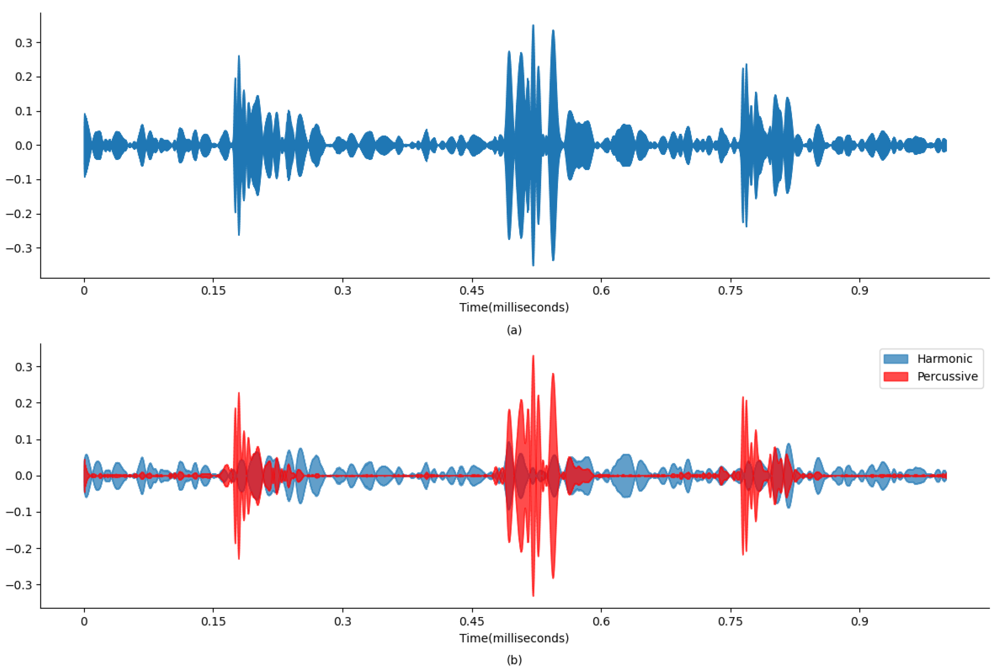
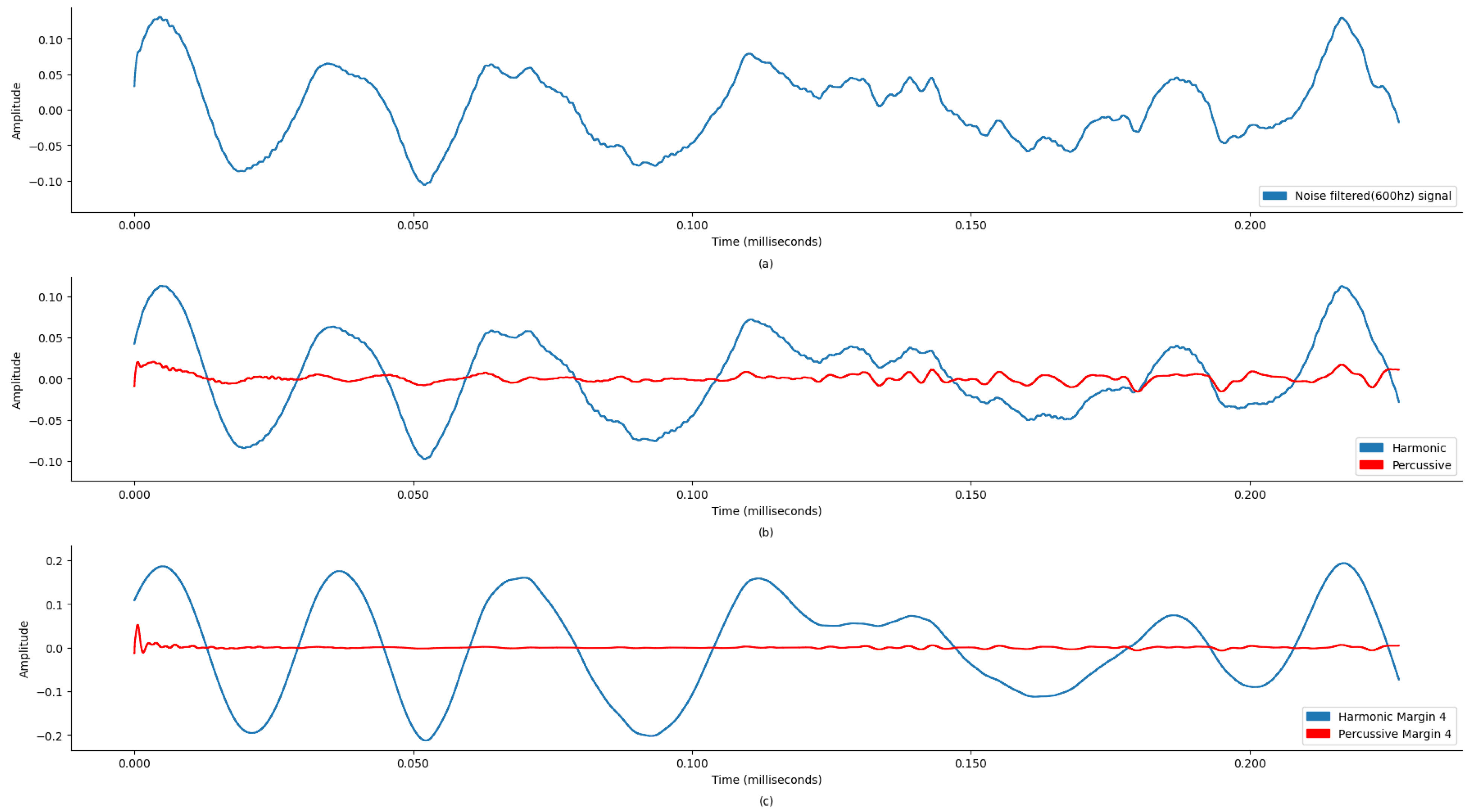
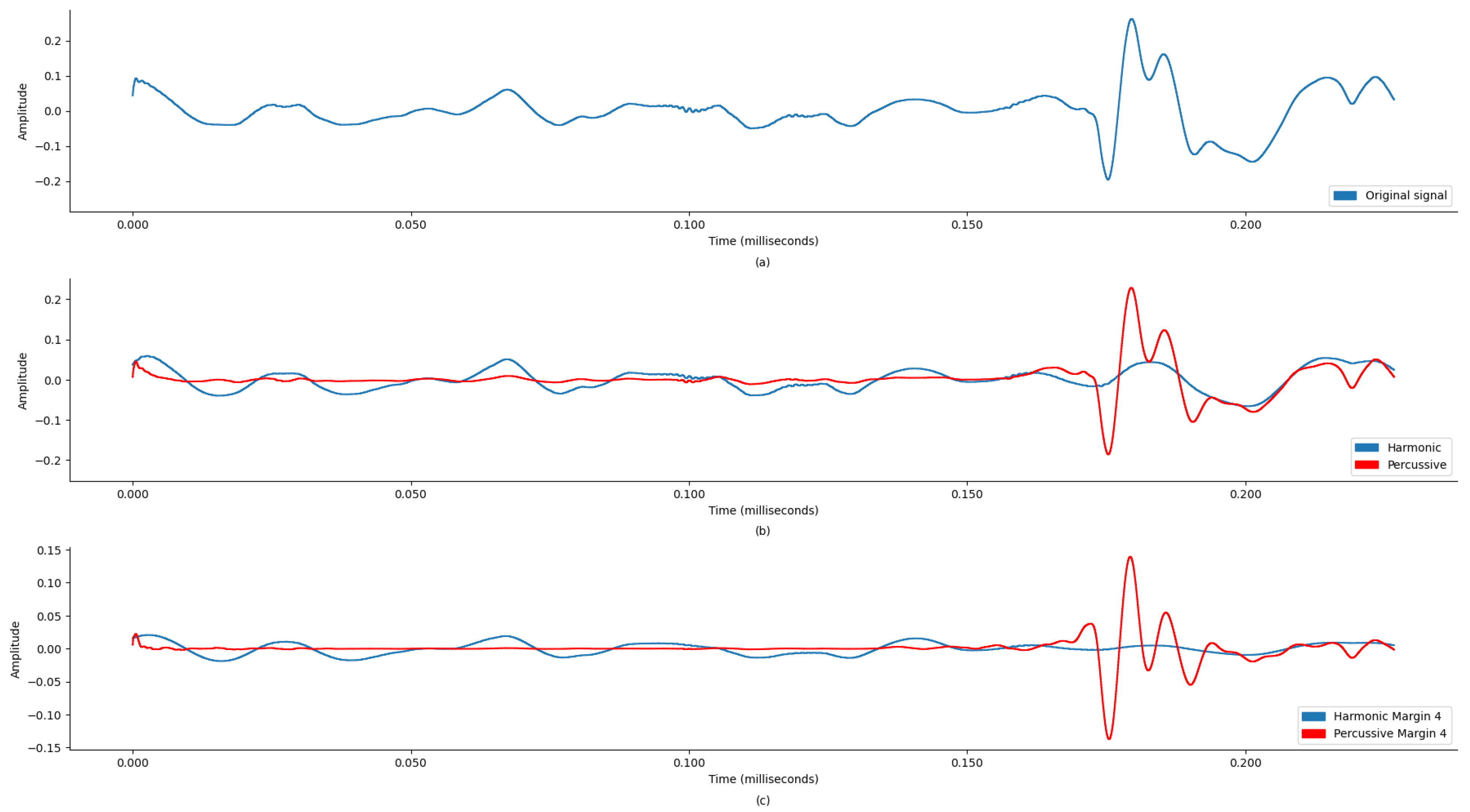
Figure 4 and Figure 5 display wave plots of normal and abnormal patient PCG samples from the dataset. Moreover, these figures display the harmonic–percussive source separation (HPSS), where harmonic and percussive sources will be further processed to extract the features from the presented PCG files for input into the ANN. The primary requirement of the challenge was to segment each sample and then develop a model to automatically classify the PCG recording as normal or abnormal. Additionally, the effectiveness of the submitted solutions was evaluated based on the sensitivity, specificity, and accuracy of the model.
Moreover, the dataset has been divided into training and test datasets, which are mutually exclusive based on the patient records. The training dataset contains the recordings from 764 patients, with 3153 recordings. The test dataset contains the mutually exclusive records from datasets ‘b’ through ‘e’ and a complete dataset from the ‘g’ and ‘i’ datasets, consisting of 308 patients with 1277 recordings. Table 3 highlights the training and test dataset record statistics [29]:
Based on the research analysis from the results reported in [29], datasets ‘b’ and ‘c’ contain the highest number of unsure recordings in both the training and test datasets. Here, the “unsure” recording label refers to audio with poor signal quality, but the dataset still contains a label for it, i.e., abnormal or normal. Also, training sets ‘a’, ‘c’, and ‘d’ contain the most abnormal cases, while training sets ‘b’, ‘d’, ‘e’, and ‘f’ contain the most normal cases. As reported in [11], the recordings labeled as abnormal may include the following pathologies: innocent or benign murmurs, aortic disease, coronary artery disease, mitral valve prolapse, and miscellaneous pathological conditions. Moreover, under pathologic recordings, the following conditions are mentioned: cardiomyopathies, congenital heart defects, arrhythmia, or valvular diseases. However, these are not specifically mentioned for each patient record.
Our study specifically excluded datasets ‘b’ and ‘c’ due to a high prevalence of recordings marked as “unsure,” which indicates poor signal quality. According to the challenge data documentation, recordings labeled as ‘unsure’ are typically characterized by significant noise and artifacts, which can compromise the reliability of machine learning models when used for classification tasks. This work chose to exclude these subsets to ensure that the training data provided a cleaner and more consistent signal, which is crucial for the robustness of our classification model. Therefore, to accommodate the optimal proportion of the abnormal and normal cases for the neural network training and to avoid overfitting, this research will use the composition of the original datasets, as mentioned in Table 4. However, the categorizations of unsure signals are highlighted in Table 5 for analysis purposes to compose a balanced dataset, while for training the model, the audio signals identified as “unsure” are included in the training, along with their designated label of abnormal or normal. Similarly, the test dataset also included the unsure records for testing the model after training.
This selection of datasets for the training of the model arguably yields a few advantages:
(a)
Through considering a training dataset with less than 10.00% of unsure recordings (i.e., dropping training datasets ‘b’ and ‘c’), training a machine learning model with higher accuracy will become much easier. Also, this research did not segment the dataset recordings, but instead directly worked on the short-term features. This reduction in unsure recordings by 3.73% facilitates more effective training of the machine learning model. This led to removing 137 patient records (521 recordings) from the training dataset and 59 patient records (219 recordings) from the test dataset.
(b)
With the exclusion of training datasets ‘b’ and ‘c’, the training and test datasets’ overall composition changed toward a more balanced set. As a result, in the training dataset, the abnormal recordings increased from 18.10% to 39.71%, and normal recordings decreased from 73.00% to 60.29%. It should be noted that 8.80% of the unsure recordings were merged into abnormal or normal classes as per the labels mentioned in the original dataset. Similarly, in the test dataset, the abnormal recordings increased from 12.00% to 36.00%, while normal recordings decreased from 77.10% to 64.00%. As in the training dataset, 10.90% of the unsure recordings of the test dataset were merged into abnormal or normal classes as per the labels mentioned in the original dataset.
(c)
With the dataset now more balanced between normal and abnormal recordings, this should discourage the neural network from overfitting the model concerning normal heart recordings and lead it toward an effective solution. Although these conditions will not prevent the model from overfitting, they will help reduce the likelihood of model overfitting.
Moreover, based on the new dataset composition, this work considered the following dataset-wise pathologies [11].

3.2. Feature Extraction and Selection

Based on the literature survey, the proposed work skipped the segmentation phase, based on the arguments of its high complexity and computation. Additionally, the research conducted by [44,45,46,47] presented valid arguments for skipping the segmentation step. The selected heart sound recording datasets from the Physionet CINC Challenge [11] were used, as discussed previously. Since the dataset was not preprocessed for noise, it was extremely important to process each recording for noise removal.
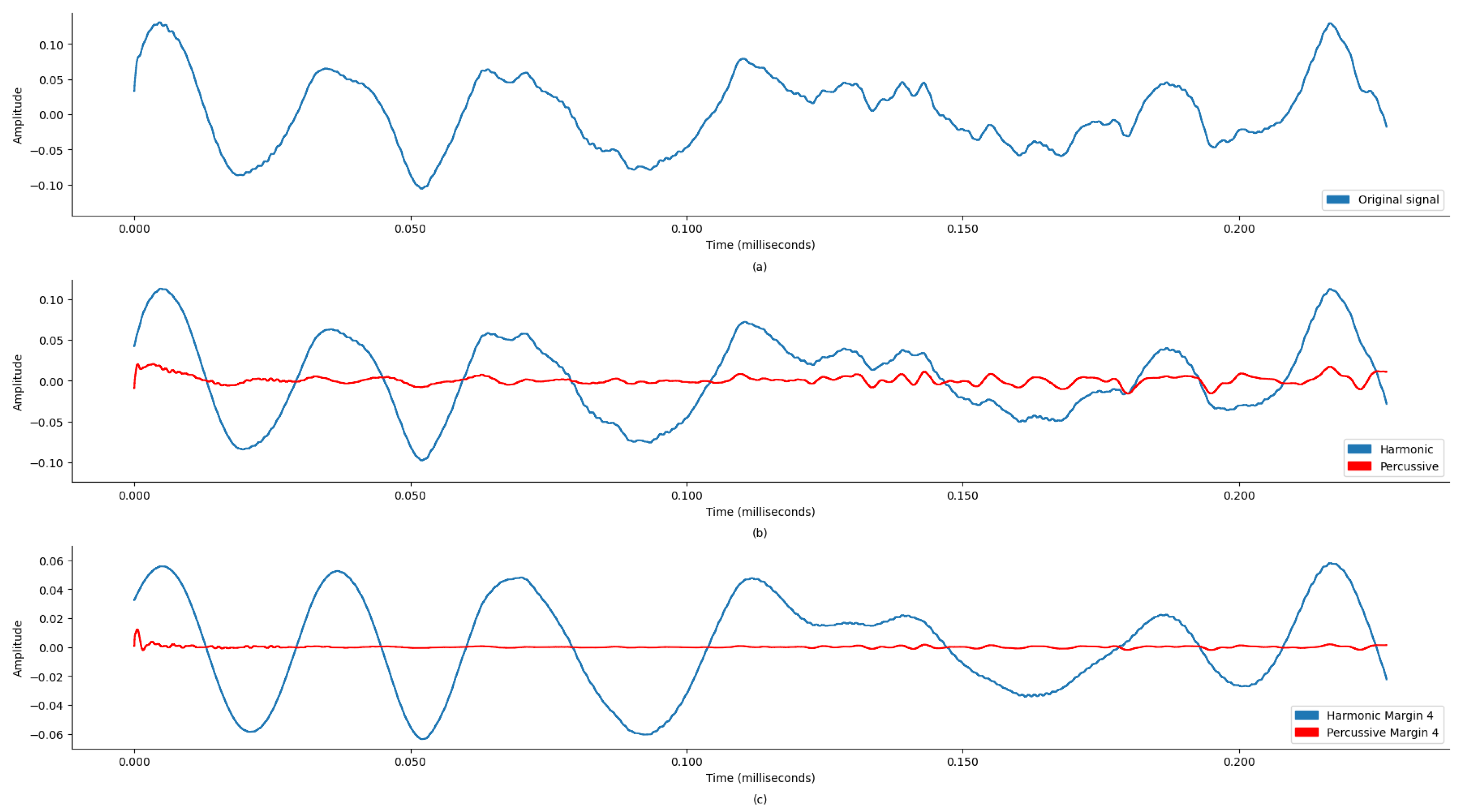
 Figure 4a and Figure 5a display the original state of the audio signal provided in the dataset. And, Figure 4b and Figure 5b display the harmonic and percussive component separation of the original audio signal, which was further processed for noise removal. Based on the findings in Table 1, the sound signal was clipped at 600 Hz.
This preprocessing step is crucial as it ensures that the subsequent audio analysis operates on cleaner, noise-reduced signals, thereby improving the reliability and accuracy of this machine learning model in detecting and classifying audio features. To enhance the quality and accuracy of the audio analysis, the preprocessing for noise reduction on the audio files was performed using thinkDSP, which is a library for systematically filtering out high-frequency noise components and other audio processing functions. This preprocessing is based on a Discrete Wavelet Transform (DWT) using the Daubechies 6 (DB6) wavelet and a threshold value of 0.1. Additionally, a low-pass filter with a 600 Hz cutoff frequency was applied for further signal refinement.
The DWT is particularly effective for analyzing non-stationary signals like PCGs because it provides a time–frequency representation, enabling localized analysis to isolate noise from the desired signal features. The DB6 wavelet, known for its compact support and orthogonality properties, was chosen for its ability to efficiently capture both smooth and transient features of the PCG signal, providing a balance between time and frequency localization. A soft thresholding technique with a threshold value of 0.1 was employed to reduce noise components while preserving the signal’s important features. The methodology involved decomposing the PCG signal using the DWT with DB6, applying the threshold to specific coefficients, reconstructing the signal using the inverse DWT, and finally applying a low-pass filter with a 600 Hz cutoff frequency to eliminate any residual high-frequency noise (Figure 3 (DWT preprocessing)).
This process reduced noise, improved the signal-to-noise ratio (SNR), and preserved essential diagnostic features. The results show that the denoised signals were diagnostically useful. This filtered signal was further processed to separate harmonic and percussive components with margin 4, enhancing the SNR and accuracy of subsequent analyses and diagnoses.
For better classification between abnormal and normal PCGs, extracting features that contain the essence of the unsegmented audio is very important. Therefore, for this work, the PCG audio files (Table 6) were processed to extract features using Librosa music and audio analysis API [48]. The feature extraction required three steps, starting with preprocessing each file for basic noise removal using the DWT, and then the denoised signal was decomposed further for HPSS with margin 4. The HPSS margin value selection was carried out through an iterative process based on preliminary experiments and performance observations. The margin value of 4 was found to provide a balanced separation between harmonic and percussive components.
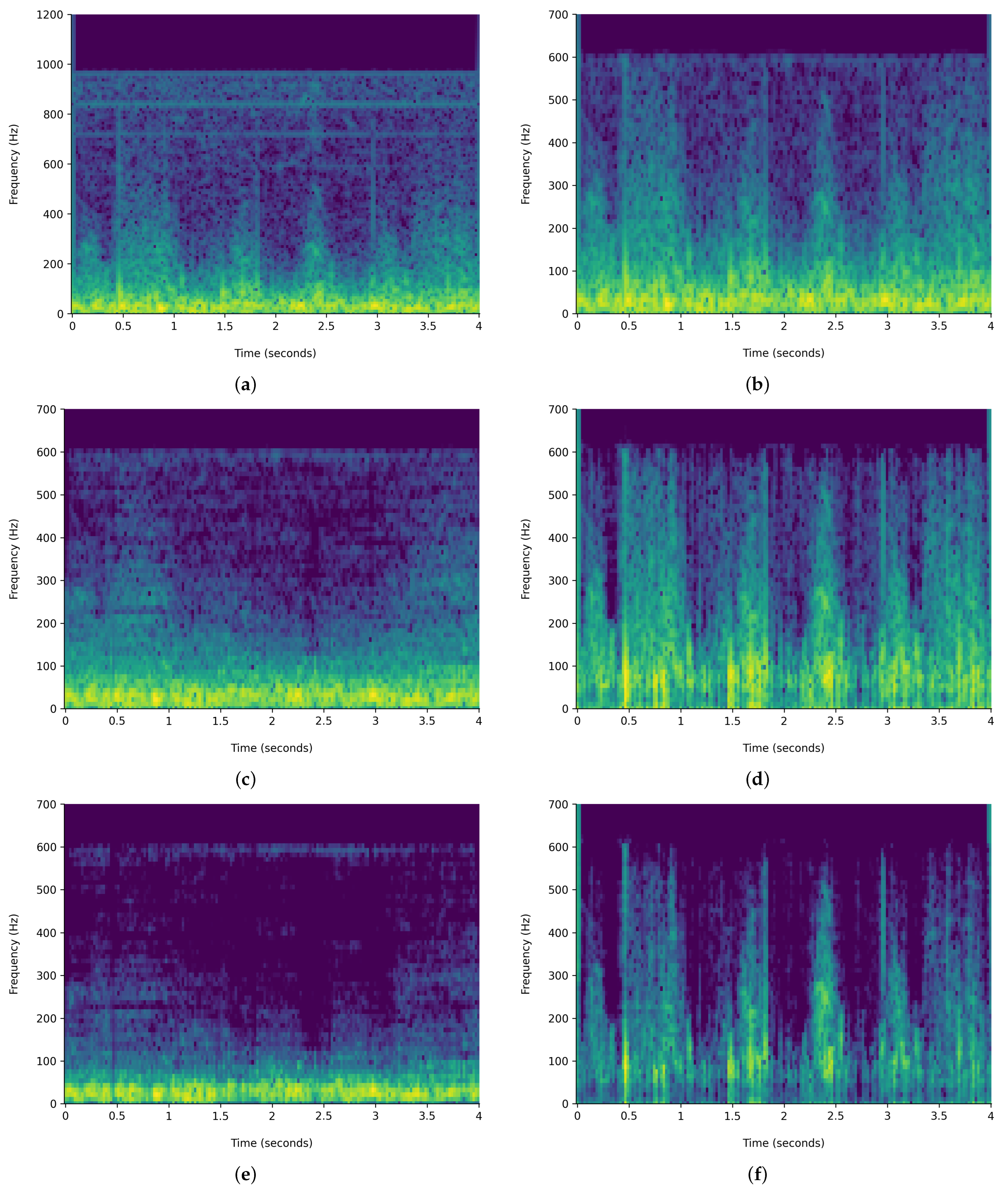
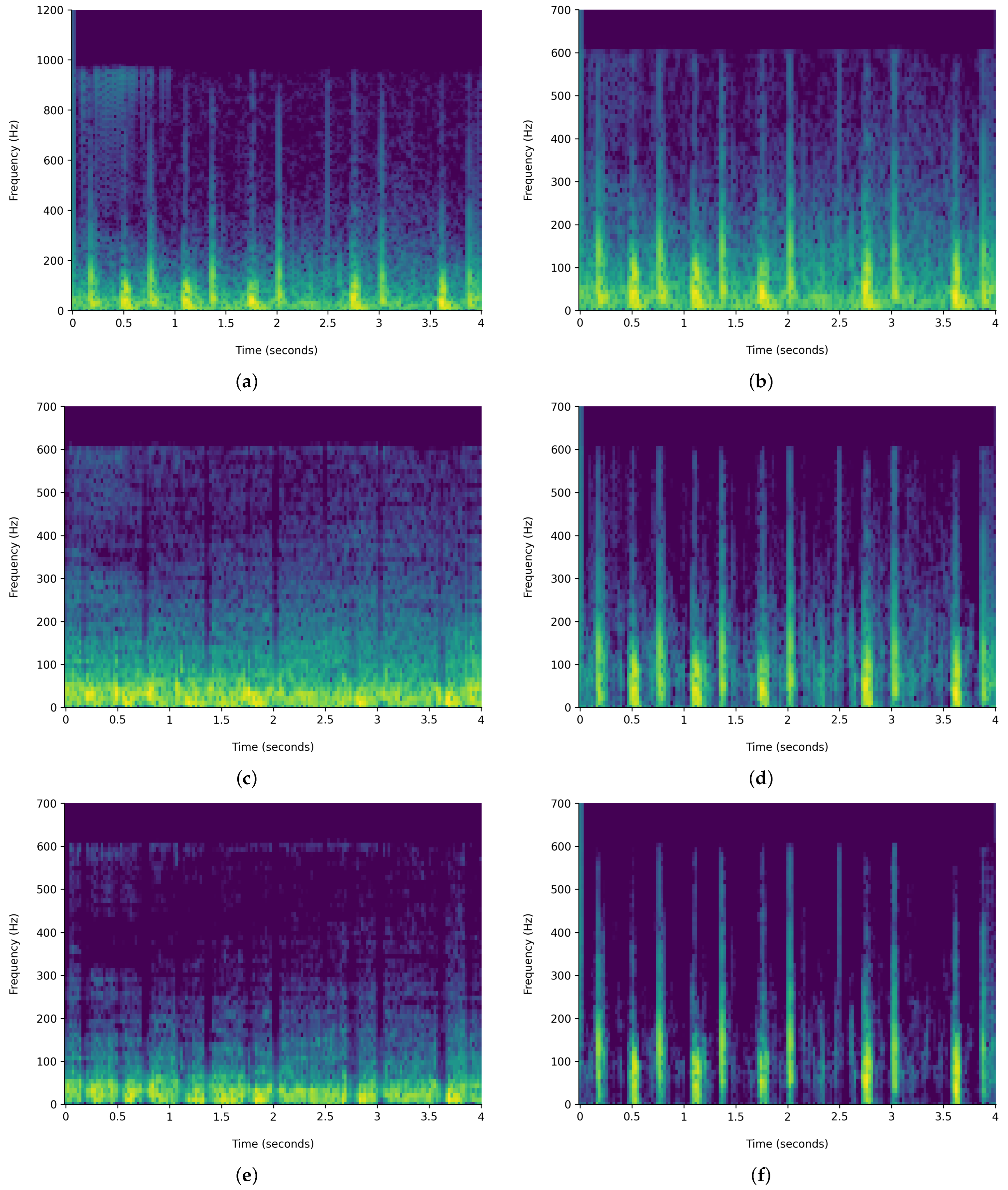
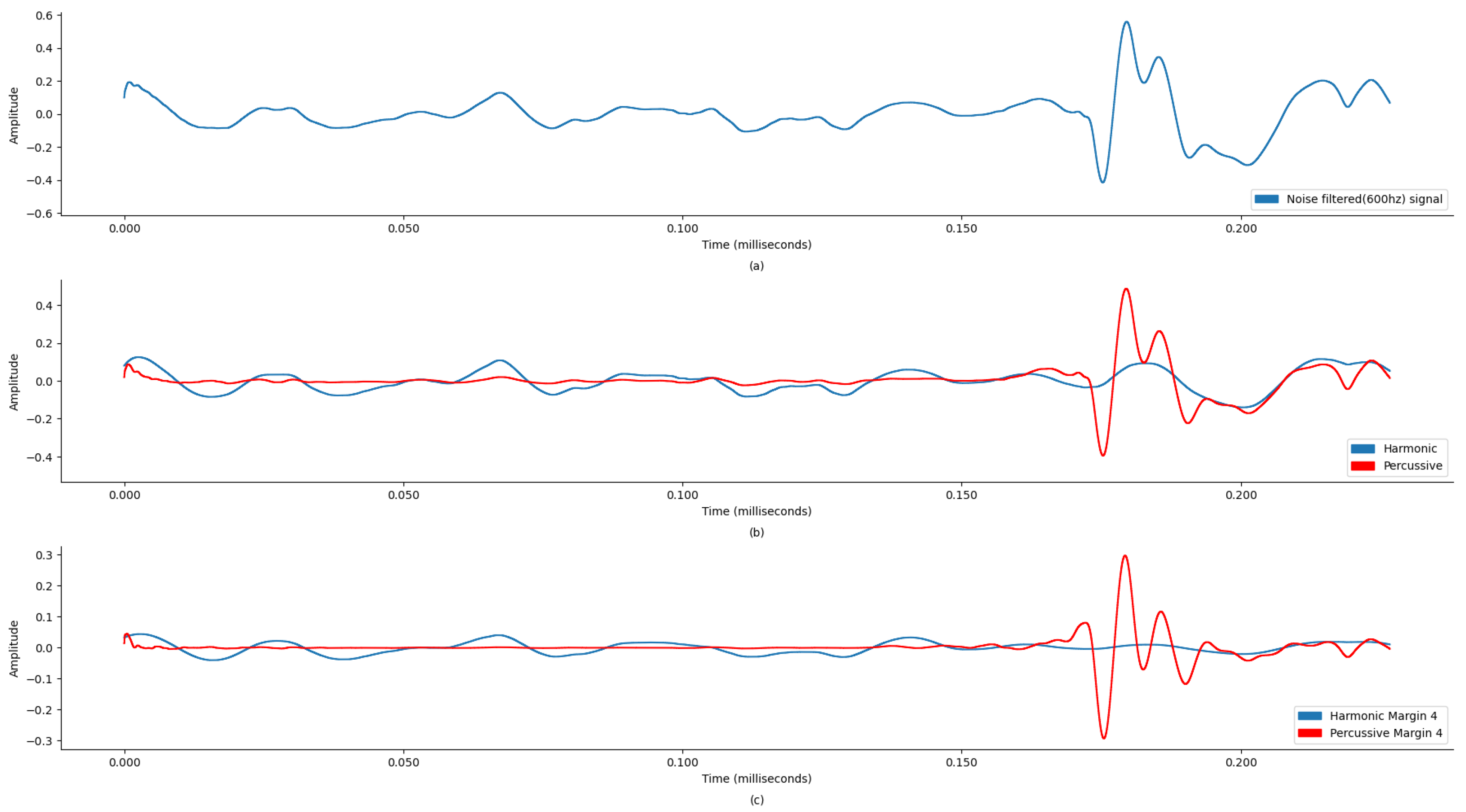
 Figure 6 and Figure 7 demonstrate the comparison of time-frequency signal representation for abnormal VS normal patients. Additionally, Figure 8 and Figure 9 demonstrate the waveplot comparison of abnormal patient HPSS original VS noise reduced PCG signal. Whereas Figure 10 and Figure 11 demonstrate the waveplot comparison of normal patients. Following this, both harmonics and percussive signals were separately processed to extract the Chroma STFT (pitch), Chroma CENS (tempo), MFCC, Chroma CQT (frequency domain), root mean square energy (signal magnitude), spectral centroid (weighted mean on the spectrum), spectral bandwidth (variance in spectral centroid), spectral roll-off, zero crossing rate (change in signal), and applicable statistical features.

3.2.1. Harmonic–Percussive Source Separation

As mentioned in the Introduction, the PCG consists of a beat rhythm with intensity variation. Therefore, extracting separate features (chroma, MFCC, etc.) based on HPSS will provide a better encoding of unsegmented audio data, potentially increasing the effectiveness of the neural network training.
The HPSS technique is particularly useful in audio signal processing, where it can enhance the analysis of audio elements by isolating the tonal and rhythmic aspects of the audio. The HPSS process involves the following steps: First, the audio signal is transformed into the time–frequency domain using a STFT. Then, the spectrogram is subjected to median filtering along the time axis to emphasize percussive components and the frequency axis to emphasize harmonic components. Finally, binary masks are created based on the filtered spectrograms to separate the harmonic and percussive components, which are then reconstructed into the time domain using an inverse STFT, displayed in Figure 6 and Figure 7. For this analysis, the margin value of 4 is used to separate harmonic and percussive components. This process is carried out using the Librosa library. The margin parameter in HPSS is used to control the sensitivity of the separation process. The margin parameter simply defines a threshold that controls how aggressively the filtering should separate the components.
A larger margin value makes the separation more tolerant, while a smaller margin value makes it more stringent. This choice of margin value in this analysis was guided by the need to achieve a more balanced separation between the harmonic and percussive elements of the PCG signals. Therefore, it was selected through an iterative process based on preliminary experiments and performance observations. PCGs typically contain both periodic heart sounds (S1, S2) and transient noise components (e.g., murmurs, clicks, etc.). Using a higher margin value ensures that subtle percussive elements, which could be indicative of pathological conditions, were adequately captured without overshadowing the harmonic components that represent the primary heart sounds.
HPSS will be effective because the harmonics will provide the pitch in audio, whereas percussive components will provide beats with localization in time. It provides an improved estimation of tempo and chroma features. Therefore, this hypothesis is based on the assumption that the features extracted from harmonic components, which detect the abnormalities in pitch, offering a better approach to detecting abnormal heart conditions in an individual patient.

3.2.2. Chroma STFT

The Chroma STFT is a powerful tool for audio signal analysis, especially in music and speech processing. At its core, the Chroma STFT was designed to capture the harmonic content of an audio signal by focusing on the relative intensity of twelve distinct pitch classes, often corresponding to the twelve traditional Western music pitches.
The primary motivation behind the Chroma STFT is rooted in the observation that many musical pieces exhibit harmonic shifts over time, but often within the same set of pitch classes. By mapping these pitch classes to a fixed set of twelve bins, regardless of the number of octaves, the Chroma STFT provides a compact representation of the audio signal’s harmonic content.
Mathematically, the Chroma STFT C of an audio signal x ( t ) can be represented as
C ( n , k ) = m = x ( m ) w ( n m ) e j ω k m
where
  • n is the time index.
  • k corresponds to one of the twelve pitch classes.
  • w ( n ) is a window function, which is typically chosen based on the application (e.g., Hamming or Hann window).
  • ω k is the angular frequency corresponding to the k-th pitch class.
The resulting Chroma STFT matrix provides a time-pitch representation, where each column corresponds to a specific time frame, and each row represents one of the twelve pitch classes. The intensity or magnitude in each cell of the matrix indicates the strength or prominence of a particular pitch class at a specific time.
By extracting the Chroma STFT feature, researchers and practitioners can profile an audio signal based on the intensity of each extracted pitch. This profiling is invaluable in various applications, including music genre classification, chord recognition, and even in some speech processing tasks where pitch and tonality play a crucial role.

3.2.3. Chroma CENS

The Chroma CENS (Chroma Energy Normalized Statistic) is an enhancement over the traditional chroma feature, aiming to provide a more robust representation of harmonic content in audio signals. The primary distinction of the Chroma CENS is its focus on short-time statistics over energy distributions within chroma bands rather than just the energy itself.
Mathematically, the Chroma CENS for a given chroma vector C can be represented as
CENS ( C ) = C μ ( C ) σ ( C )
where
  • C is the chroma vector, typically obtained from the Chroma STFT or a similar method.
  • μ ( C ) is the mean energy of the chroma vector over a short time window.
  • σ ( C ) is the standard deviation of the energy of the chroma vector over the same window.
Through normalizing the chroma vector in this manner, the Chroma CENS effectively reduces the influence of dynamics (loudness variations) and timbral characteristics, focusing primarily on the harmonic content. This normalization process ensures that the resulting feature is less sensitive to variations in dynamics, recording conditions, or specific instrument timbres, making it particularly robust for tasks like music similarity and retrieval.
The low temporal resolution of the Chroma CENS is intentional. By averaging out the chroma values over longer time frames, it captures the essence of the harmonic progression while being less affected by short-term fluctuations or transients. This makes the Chroma CENS efficient for extracting stable harmonic features from the audio, providing a summarized yet informative representation of the audio’s tonal content.

3.2.4. Chroma CQT

The Chroma CQT (Chroma Constant-Q Transform) is designed to extract chroma features from an audio signal using a logarithmically spaced frequency axis. The Constant-Q Transform is unique in that it provides a constant ratio between the center frequencies of adjacent filters, making it particularly suited for musical/non-stationary signals, where pitches are often geometrically spaced.
The formula for the Constant-Q Transform is given by
C Q T k ( t ) = n = x [ n ] · e j ω k n · w k [ n t ]
where
  • x [ n ] is the audio signal.
  • ω k is the center frequency of the k-th filter, determined by the geometric spacing.
  • w k [ n t ] is the window function for the k-th filter, which is typically designed to have a constant Q value, where Q is the ratio of the center frequency to the bandwidth.
The Chroma CQT then maps the resulting spectrum from the CQT onto 12 chroma bands corresponding to the 12 pitch classes. This is achieved by summing the energies in the CQT bins that correspond to the same pitch class, regardless of the octave.
The logarithmically spaced frequency axis of the CQT ensures that each octave is represented with an equal number of filters, aligning well with the perception of pitch in human hearing. This makes the Chroma CQT an effective tool for capturing the harmonic and melodic content, providing a meaningful and computationally efficient representation.

3.2.5. MFCC

The application of Mel-frequency cepstral coefficients (MFCCs) is prevalent in speech and audio processing. The auditory features are obtained from the spectral information of an audio signal and are specifically engineered to replicate the human ear’s non-linear auditory perception of sounds. The process of computing MFCCs involves several steps:
  • Fourier Transform: The audio signal is first transformed into the frequency domain using a Fourier transform:
    X ( f ) = x ( t ) e j 2 π f t d t
    where x ( t ) is the time-domain audio signal, and X ( f ) is its frequency representation.
  • Mel Filterbank Processing: The magnitude spectrum obtained from the Fourier transform is then passed through a series of overlapping filters, typically triangular and spaced uniformly on the Mel scale. The Mel scale is a perceptual scale that approximates the human ear’s response to different frequencies. The output of this stage is the energy in each Mel filter:
    E m = f = 1 F | X ( f ) | 2 H m ( f )
    where H m ( f ) is the m-th Mel filter, and F is the total number of frequency bins.
  • Logarithmic Compression: The energies from the Mel filterbanks are log-transformed to mimic the logarithmic perception of amplitude and loudness in human hearing:
    L m = log ( E m )
  • Discrete Cosine Transform (DCT): Finally, the MFCCs are obtained by taking the Discrete Cosine Transform of the log energies. This step decorrelates the filterbank coefficients and yields a compressed representation of the filterbank energies:
    M F C C k = m = 1 M L m cos π k ( m 0.5 ) M
    for k = 1 , 2 , , K , where M is the number of Mel filters, and K is the desired number of MFCCs.
For the research in context, a filter bank with 40 Mel filters was utilized, implying that M = 40 in the above equations.
MFCCs are widely preferred in various audio and speech-processing applications because of their capability to capture the phonetically significant attributes of an audio signal while also exhibiting resilience against specific signal changes.

3.2.6. Root Mean Square Energy

The root means square energy (RMSE) feature uses a spectrogram to extract the information on signal energy over time. To extract the RMSE, this research work used a frame length of 2048 and a hop length of 512, where frame length is the size of samples from the audio signal used for energy calculation and hop length for performing an intermediate STFT. The RSME is defined as
1 N n | x ( n ) | 2

3.2.7. Spectral Centroid

This is a simple measure based on the spectral position and shape. The centroid provides the center of the gravity/mass of the signal spectrum and is calculated based on frames. A general observation is that the greater the value presented, the more prominent the sounds.
C i = n = 0 N 1 f ( n ) x ( n ) n = 0 N 1 x ( n )
where x ( n ) represents the weighted frequency value, or magnitude, of bin number n, and f ( n ) represents the center frequency of that bin.

3.2.8. Spectral Bandwidth

This is the difference between the upper and lower frequencies in a continuous band of frequencies. This feature identifies the frequency range for PCGs. Librosa computes the p-order spectral bandwidth, and it is defined by
k S ( k ) ( f ( k ) f c ) p 1 p
where S ( k ) is the spectral magnitude at frequency bin k, f ( k ) is the frequency at bin k, and f c is the spectral centroid. When p = 2, this is like a weighted standard deviation.

3.2.9. Spectral Roll-Off

This is a spectral shape descriptor used to discriminate between different audio spectra. This audio feature defines the frequency below which the max percentage of the magnitude distribution of the spectrum is concentrated. This work used the Librosa library and used 85.00% as the roll percentage.
k = 1 m X i ( k ) = 0.85 k = 1 W f L X i ( k )
The spectral roll-off frequency is usually normalized by dividing it by W f L , so that it takes values between 0 and 1. This type of normalization implies that a value of 1 corresponds to the maximum frequency of the signal, i.e., to half the sampling frequency.

3.2.10. Zero Crossing Rate

This is the rate of change in the sign of the signal during the frame, or it can be said to be the frequency of change in sign in a signal divided by the length of the frame. It is defined as
Z ( i ) = 1 2 W L n = 1 W L | s g n [ x i ( n ) ] x i ( n 1 ) |
where the sgn function is defined as
s g n [ x i ( n ) ] = 1 x i ( n ) 0 1 x i ( n ) < 0

3.2.11. Statistical Features

Mean

This is the signal’s average amplitude over a considered time interval. This feature is considered because the mean value of abnormal PCGs vs. normal PCGs is higher. It is defined by
μ = 1 N i = 0 N 1 x i
where x i represents ith amplitude instance in the signal, and N is the total number of instances.

Mode

The mode is a fundamental measure of central tendency that identifies the value or values that occur most frequently within a dataset. Unlike the mean and median, which provide a numerical average or a central value, respectively, the mode offers insights into the most common or repetitive patterns in the data.
There are a few key characteristics of the mode:
  • It directly reflects the highest peak of the data distribution, indicating where data samples are most densely concentrated.
  • A dataset can have one mode (unimodal), more than one mode (bimodal or multimodal), or no mode at all.
  • The mode is particularly robust against outliers or extreme values. Since it is based solely on the frequency of occurrence, it remains unaffected by the magnitude of data points, making it a reliable measure in datasets with potential anomalies.
In the context of signal analysis, the mode becomes especially pertinent. Given that signals often contain repetitive patterns or recurring values, identifying the mode can provide insights into the inherent characteristics or the “essence” of the signal. For instance, in medical signal analysis, the mode can help differentiate between normal and abnormal signals by highlighting the most common patterns present. If a particular value or pattern frequently appears in a normal signal but is absent or less frequent in an abnormal one, the mode can be a distinguishing feature.
By incorporating the mode as a feature in the analysis, this work aimed to harness its resilience against extreme values and its ability to capture the core patterns of the signal. This ensures a more accurate and reliable differentiation between different classes or categories of signals, enhancing the overall efficacy of the analysis.

Median

The median is a central measure of tendency that provides significant insights into the distribution of a dataset. Unlike the mean, which takes into account all values in a dataset, the median focuses solely on the middle value, making it resistant to outliers or extreme values. This characteristic ensures that the median provides a more robust representation of the central location of data, especially in skewed distributions.
In a dataset arranged in non-decreasing order, we have the following:
  • If the number of observations, denoted as n, is odd, then the median is the value at the exact middle position, which can be mathematically represented as the value at the ( n + 1 ) / 2 th position.
  • If n is even, the median is typically calculated as the average of the two middle values, specifically the values at the n / 2 th and ( n / 2 ) + 1 th positions.
By this definition, exactly 50.00% of the observations in the dataset lie below the median, and the remaining 50.00% lie above it. This property makes the median a particularly valuable metric in understanding the central tendency of a dataset, as it divides the dataset into two equal halves in terms of the number of observations, regardless of the actual values of those observations.
Given its resistance to extreme values, the median is often preferred over the mean in datasets that may contain outliers or when the distribution of data is notably skewed. It clarifies “typical” values in such scenarios, ensuring that a few extreme observations do not unduly influence the central tendency.

Standard Deviation

This is an important statistical feature that helps determine how much the sample under process deviates from its mean value. A higher standard deviation indicates that the data are spread over a wider range, whereas a lower deviation means the data points are closer to the mean. This helps differentiate between normal and abnormal PCGs.
1 N 1 n = 1 N ( x n μ ) 2
Here, N represents the total number of observations; μ represents the mean of the given data; and x n is the value of each amplitude point considered.

Skewness

The primary purpose of using skewness is to determine whether the sample under process is normally distributed or not. A normally distributed sample will have zero skewness, whereas if it is left- or right-distributed, then the sample is asymmetrical and points out to be an abnormal PCG.
i = 0 N ( X i μ ) 3 ( N 1 ) . σ 3

Quantile25

The 25th percentile, often referred to as the first quartile or Quantile25, is a statistical measure that provides insights into the distribution of data in a dataset. It represents the value below which 25.00% of the observations can be found. In other words, it is the value at which one-quarter of the data lie below it, serving as a marker that separates the lowest 25.00% of the data from the rest.
To compute the Quantile25 for a given dataset, we have the following steps:
  • First, the data points are sorted in non-decreasing order.
  • Then, the position p is calculated using the formula
    p = n + 1 4
    where n is the total number of data points in the dataset.
  • If p is an integer, then the data point at position p is the 25th percentile.
  • If p is not an integer, then the 25th percentile is typically computed by linear interpolation between the data points at positions p (the largest integer less than or equal to p) and p (the smallest integer greater than or equal to p).
Thus, Quantile25 serves as a threshold, distinguishing the lower quarter of data points from the upper three-quarters in terms of magnitude.

Quantile75

The 75th percentile, often referred to as the third quartile or Quantile75, is a statistical measure that delineates the distribution of data in a dataset. It represents the value below which 75% of the observations fall. In essence, it is the value at which three-quarters of the data lie below it, serving as a boundary that separates the lowest 75% of the data from the highest 25%.
To compute the Quantile75 for a given dataset, we have the following steps:
  • Initially, the data points are sorted in non-decreasing order.
  • Subsequently, the position p is determined using the formula
    p = 3 ( n + 1 ) 4
    where n denotes the total number of data points in the dataset.
  • If p is an integer, then the data point at position p is the 75th percentile.
  • If p is not an integer, then the 75th percentile is typically derived by linear interpolation between the data points at positions p (the largest integer less than or equal to p) and p (the smallest integer greater than or equal to p).
Thus, Quantile75 acts as a demarcation, distinguishing the lower three-quarters of data points from the uppermost quarter in terms of magnitude.

IQR

The Interquartile Range, commonly abbreviated as IQR, is a robust measure of statistical dispersion or spread in a dataset. It specifically describes the range within which the central 50% of values lie when the data are ordered from the lowest to the highest value. By focusing on the middle 50%, the IQR effectively eliminates the influence of extreme values or outliers, making it a particularly valuable metric in datasets that may contain such anomalies.
Mathematically, the IQR is the difference between the third quartile (Quantile75) and the first quartile (Quantile25). It can be represented by the formula
IQR = Quantile 75 Quantile 25
Given that Quantile75 represents the value below which 75% of the data fall, and Quantile25 represents the value below which 25% of the data fall, their difference (IQR) encapsulates the range of the middle 50% of the data. This range is particularly significant in statistical analyses as it provides insights into the variability and spread of the central portion of the dataset, excluding potential outliers.
In many statistical applications, the IQR is used in conjunction with other metrics, such as the median, to provide a comprehensive understanding of the data distribution. Moreover, the IQR is frequently employed to identify outliers. Observations that fall below Quantile 25 1.5 × IQR or above Quantile 75 + 1.5 × IQR are typically considered outliers, as they lie outside the range expected for the central bulk of the data.

Kurtosis

This significant statistical feature provides information about the signal distribution within the data sample. This feature helps in detecting the high-amplitude peaks in the PCG signal, which is beyond a threshold point and indicates an abnormal heart condition. This is formulated as
i = 0 N ( X i μ ) 4 ( N 1 ) . σ 4
In the research referenced in the literature, features are extracted on a per-second basis. They are only extracted from a part of the audio file, i.e., 3 to 8 s only. However, when training a simple sequential artificial neural network, it was observed that the number of records was not adequate. Therefore, for this work, features were extracted on a per-second basis for the full duration of each PCG file. This results in an increase of 3.5 times in the total record of the extracted feature set dataset, further aiding the effective training of a neural network and improving the classification of abnormal cases. Precisely, the data were extracted with dimensions of 164 feature columns and 65,940 rows in comparison to 19,034 rows based on 7 s of audio.
The next step is feature selection, which is performed based on a careful analysis of the reviewed literature. In this study, the ROC-AUC method [49], along with the count of features, was employed for feature selection to prioritize those features that exhibit strong discriminatory power between normal and abnormal PCG signals. Various feature set combinations were manually evaluated and selected (Table 7) by observing their individual contributions to classification accuracy, using ROC-AUC scores to select the top-performing features. This step involved evaluating feature sets in a systematic manner to ensure a balanced representation of harmonic and percussive characteristics.
The choice of ROC-AUC over other feature selection techniques such as PCA, Ranker and Info Gain [42], and the Wilcoxon method [49] was driven by its ability to directly evaluate the classification performance of individual features across varying thresholds. Unlike PCA, which focuses on dimensionality reduction through linear combinations of features, ROC-AUC provides a more interpretable and the direct assessment of each feature’s relevance to the binary classification task. Additionally, while Ranker and Info Gain assesses feature importance based on information gain, and the Wilcoxon method evaluates features based on statistical significance, ROC-AUC offers a more holistic approach by considering both true positive and false positive rates. This method ensures that selected features contribute to model accuracy and overall balance between sensitivity and specificity, which is critical for reliable medical diagnostics.

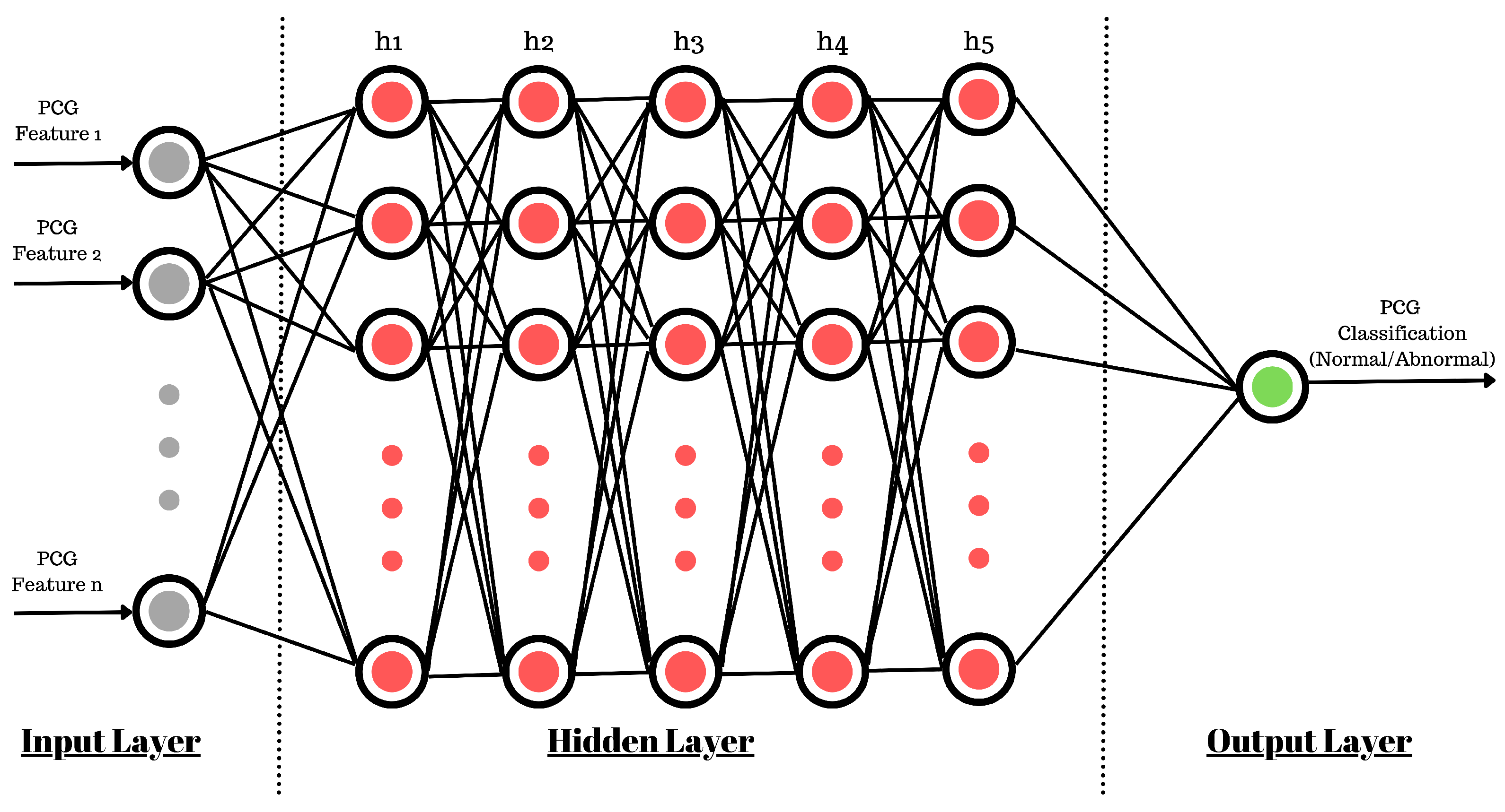
3.3. Feed-Forward Artificial Neural Network

An ANN is a simplified mathematical model consisting of artificial neuron functions that imitate the behavior of human brain neurons. This work utilized the power and simplicity of feed-forward neural networks implemented using the TensorFlow Keras library. Multiple hyperparameter tunings were performed, as mentioned in Table 8, and these are discussed further.
The use of a sequential model (Figure 12) allows us to create five hidden layers of neurons with a density of 512 neurons at each inner layer. For the smooth training of the ANN model, the learning rate was kept at 1 × 10 5 (0.00001). This controls the rate at which the model adapts to the problem at hand. The learning rate is one of the most important parameters used to control the rate of change in neuron connection weights. If it is too large, it will quickly converge to a suboptimal solution, or if it is too small, then it can cause the process to stall. Therefore, identifying a trade-off value is important and may require multiple runs of model training. Also, based on the feature selection discussed in the previous section, the input shape for the ANN varies for each experiment.
Before the start of the ANN training, the neuron connection weights must be initialized. This work utilized a random uniform initializer for model weights in the range of −0.05 to +0.05. Accordingly, the weights were uniformly distributed, ensuring that each weight had an equal chance of being assigned any value between the minimum and maximum. This helped prevent overfitting and enabled the network to converge more quickly to an optimal solution. Ultimately, this impacted the outcome of the optimization procedure of the ANN and its ability to generalize based on the problem.
Now, because initializers were used, the ANN may have become sensitive to initial random weights, which may lead to slow model convergence. To counter this, a batch normalization layer was used, which normalizes the inputs to a layer for each batch of inputs. It helps reduce the internal covariate shift, thereby speeding up the learning process and reducing the chances of overfitting. Batch normalization also helps reduce the vanishing/exploding gradients problem and improves generalization ability. This leads to stable model training due to regularization, fewer generalization errors, and reduced training epochs, resulting in accelerated learning.
For each neuron in the hidden layers, the ReLU activation function was used to introduce non-linearity into the network. ReLU is computationally efficient, prevents the neural network from becoming saturated, and helps to train the model faster. It is utilized to overcome the vanishing gradient problem as well as for faster computations.
Since this work performed the classification of PCGs as normal or abnormal, the final layer contains only one neuron with a sigmoid activation function. For overall model learning adaptation, the Adamax optimizer was utilized; it extends the functionality of the Gradient Descent Optimization algorithm, inherently accelerating the optimization process. Adamax is a variant of the popular Adam optimization algorithm and is often preferred for training deep neural networks. It combines the advantages of the AdaGrad and RMSprop algorithms, both of which maintain per-parameter learning rates and update parameters based on adaptive learning rate methods. Unlike those algorithms, however, Adamax uses the infinity norm rather than the Euclidean norm to calculate parameter updates. This allows it to better handle sparse gradients, making it more suitable for training deep neural networks with a large number of parameters and layers. Additionally, Adamax uses a combination of momentum and decay rates to improve convergence while maintaining stability. This makes it well suited for heart sound classification. Finally, the computing loss during the model training process was calibrated through binary cross entropy.
These data were not yet ready to be fed directly to the neural network, so the dataset was further processed to remove the outlier records. This study used the Interquartile Range (IQR) method to detect and remove outliers from the dataset. For each feature, the first quartile (Q1) and third quartile (Q3) were calculated, with the IQR defined as Q3 − Q1. Data points outside the range of Q1 − 1.5 × IQR to Q3 + 1.5 × IQR were considered outliers and removed. This method, which is robust to non-normal data distributions, helped ensure that only statistically relevant data remained for model training, thereby improving classification accuracy. These exercises help prevent models from being over/underfit. After outlier removal, the dataset was reduced from 65,940 to 37,243 rows, which is still a decent volume of data that can be used to train a neural network. Going forward, these data were split into test and training sets with a ratio of 10:90 for the training of the neural network. This was carried out separately based on the classification category (normal/abnormal). This activity helped maintain the effectiveness of the model training and the model’s testing on unseen data.

4. Results and Discussion

The experiments conducted to test this hypothesis were based on feeding the data of extracted features to the sequential feed-forward artificial neural network. The limitation of this method is the manual selection of feature sets for model training, which can be automated with the help of various feature selection techniques and variations in the neural network models. Based on the results, accuracy levels were tested across different feature sets from the PCG dataset.

4.1. Evaluation Parameters

According to the literature review in the field of PCG analysis using an ANN, a comprehensive evaluation necessitates the use of three primary metrics, namely, accuracy, sensitivity, and specificity [21].
Accuracy serves as a pivotal metric, providing a snapshot of the model’s performance by determining the proportion of correct predictions made out of the total predictions. However, with the potential for class imbalance in PCG datasets, the metric’s effectiveness may be compromised, necessitating further evaluation.
A c c u r a c y = T P + T N T P + T N + F P + F N
Sensitivity, or the true positive rate, steps in to address this, providing a measure of the model’s capability in correctly identifying actual heart anomalies, thereby minimizing false negatives. This becomes imperative when dealing with critical health-related outcomes, where overlooked cases could lead to serious misdiagnoses.
S e n s i t i v i t y = T P T P + T N
Specificity complements sensitivity, focusing on the model’s ability to accurately identify normal cases, thereby minimizing false positives. This is essential to reducing unnecessary medical interventions based on inaccurate diagnoses.
S p e c i f i c i t y = T N T N + F P
Here, TP: true positive; TN: true negative; FP: false positive; FN: false negative. It is crucial to consider these metrics holistically. A model may exhibit high accuracy but compromise on sensitivity, thereby frequently misclassifying positive instances. Alternatively, a model demonstrating high sensitivity but low specificity may contribute to excessive false positives. Therefore, this triad of metrics fosters a nuanced understanding of the model’s performance, providing valuable insights to drive refinements in subsequent iterations.

4.2. Model Training and Results

The ANN training was performed multiple times to check the effectiveness of various combinations of features extracted from the PCG signal. As mentioned, there are a total of 164 features. The training was performed based on harmonics and percussive features. Harmonic features of a PCG are related to the sound of the heartbeat itself, such as the rate and rhythm. Percussive features are related to the timing and intensity of the heartbeat, for example, the timing of systole and diastole. The hypothesis was tested with both the harmonic and percussive features, and it was found that with the current ANN setup, the harmonic-based features performed well with an accuracy between 92.00% and 94.00%. This work tried using PCA and ICA techniques, but the results were not encouraging. Therefore, the approach was changed to analyze the features individually based on their harmonic and percussive components separately. Thus, a manual “sequential search method” was used, where features were added or removed from the set one at a time based on the model performance until the optimal set of features was found. Therefore, no specific feature selection method is mentioned in the manuscript.
Also, Table 9 presents the set of records demonstrated in the confusion matrix for harmonic features (Figure 13).

4.3. Harmonic Feature Test

This work tested various combinations of 12 chroma, 12 Chroma CENS, 40 MFCC, and 18 statistical harmonic features. The model performances are listed in Table 7, along with the confusion matrix in Figure 13 and the respective ROC in Figure 14.
For harmonic features, the following combinations were tested: chroma only, Chroma CENS only, MFCC only, statistical only, chroma + statistical, Chroma CENS + statistical, MFCC + statistical, and all feature combinations. While the combinations of all the harmonic features produced a validation accuracy of 93.80%, the chroma harmonic features produced a validation accuracy of 93.40%. Compared to all feature combinations, the chroma-only experiment observed that the recall for normal label falls by 0.01 and for abnormal label precision, the F1-score falls by 0.01. This resulted in a fall in accuracy of 1.00%. This is a significant change, yet the chroma features performed well, with only 12 features compared to 82 in the previous test. Additionally, the 18 statistical features performed well in the validation accuracy with 92.70% but showed a slight drop in performance for the abnormal label.
The Chroma CENS harmonic features produced a validation accuracy of 80.30%, which is 13.10% less than the chroma-only features. Additionally, for the abnormal label, it did not perform well. On the other hand, the MFCC harmonic features produced a validation accuracy of 92.60% and performed fairly well on normal labels. However, abnormal labels, showed significantly lower recall metrics.
The combination of chroma and statistical harmonic features produced a validation accuracy of 92.90%. It was observed that the recall and F1-score for the abnormal class dropped by 0.04 and 0.02 points. Additionally, for the normal class, the precision fell 0.01 points. Meanwhile, a combination of the Chroma CENS and statistical harmonic features produced a validation accuracy of 92.40%, which is a significant improvement in comparison to Chroma-CENS-only features. In comparison to all the features, it was observed that the recall and F1-score for an abnormal class dropped by 0.04 and 0.02 points. Also, for the normal class, the precision fell by 0.01 points.
Finally, the combination of MFCC and statistical harmonic features produced a validation accuracy of 93.50%. It was observed that the abnormal class precision, recall, and F1-score improved and were close to the full harmonic feature set, but compared to the chroma-only feature test, it required more computations.

4.4. Percussive Feature Test

Various combinations of 12 chroma, 12 Chroma CENS, 40 MFCC, and 18 statistical percussive features were tested. The model performances are listed in Table 10, along with the confusion matrix in Figure 15 and the respective ROC in Figure 16.
For percussive features, the chroma only, Chroma CENS only, MFCC only, statistical only, chroma + statistical, Chroma CENS + statistical, MFCC + statistical, and all feature combinations were tested. The validation accuracy ranged from 80.00% to 91.00%. The range of accuracy compared to the harmonic feature combinations is significantly lower and unacceptable for the machine diagnostic parameters.
Here, among the combination of all percussive features, only MFCC and MFCC + statistical features produced a validation accuracy of 90.70% and 91.00%. In comparison to this, chroma only, Chroma CENS only, and both combined with statistical percussive features produced validation accuracies of 80.50%, 80.30%, 85.80%, and 80.30% only.
Moreover, except for the MFCC + statistical percussive features, all other combinations did not work well in predicting the abnormal class.
Also, Table 11 presents the set of records demonstrated in the confusion matrix for harmonic features (Figure 15).

4.5. Result Comparison

The present study compared the accuracy, specificity, and sensitivity of different combinations of percussive and harmonic features, as illustrated in Table 12. However, based on the ROC-AUC feature selection method, the findings demonstrate that the chroma-based harmonic features yield the most favorable outcomes. Comprising only 12 attributes, they still demonstrated remarkable efficiency, achieving a classification accuracy of 93.40%, sensitivity of 82.40%, and specificity of 80.60%. This reduced feature set notably lowers the computational load, enabling faster training and testing while maintaining diagnostic reliability. The ANN model achieved up to 93.80% accuracy, with 82.50% sensitivity and 82.40% specificity, using the full harmonic feature set, which comprised 82 features, underscoring the robustness of the selected attributes. However, using a reduced feature set, particularly focusing on the 12 chroma features, provides significant computational benefits, especially during real-time testing and application in clinical settings. Through focusing on a smaller number of features, the computational load decreases, making the model more efficient and suitable for deployment on devices with limited processing capabilities, such as mobile health monitoring tools or embedded systems. This efficiency can lead to faster processing times, allowing for rapid and near-real-time classification of heart sounds [40].
Moreover, the chroma features mitigate this limitation by effectively representing harmonic content from the PCG signals. Chroma features focus on the pitch content and emphasize harmonics that are crucial for distinguishing between normal and abnormal heart sounds. This makes them particularly effective in capturing the key spectral qualities required for accurate classification, even with a reduced set of features. Additionally, removing low-quality signals and balancing class distributions further enhanced the model’s effectiveness in real-world scenarios. This study emphasizes the potential for deploying such computationally efficient, non-invasive diagnostic models in resource-constrained environments, paving the way for advancements in cardiac health monitoring.
Table 13 provides a comparison of previous studies and the proposed work.

5. Conclusions

Based on the experiments performed and in using the various combinations of harmonic and percussive feature sets, harmonic features outperformed percussive features for the balanced prediction of both normal and abnormal labels.
It can be concluded that the expert system, implemented using a feed-forward neural network with four hidden layers and one output layer, using the TensorFlow Keras library, has shown promising results for classifying normal and abnormal heart sounds. The hyperparameters, such as learning rate and batch size, were tuned to obtain the best performance of the model. The use of a sequential model allowed for the creation of multiple hidden layers with a high density of neurons, contributing to the overall performance of the model.
Moreover, using the Adamax optimizer, a variant of the Adam optimization algorithm proved to be effective in accelerating the optimization process, improving convergence and maintaining stability during training. Additionally, using ReLU activation functions for hidden layers, batch normalization layers and binary cross-entropy loss during the training process contributed to the stability, accuracy, and the generalization ability of the model.
Even though the combinations of all 82 harmonic features achieved a maximum validation accuracy of 93.80%, considering the overall computational complexity, the PCG classification experiment based on 12 chroma harmonic features can also be considered for a better computation performance, where the accuracy is 93.40%, and the area under the curve (AUC) is 0.975, which is good.
This work tested the ANN using the PhysioNet Challenge dataset, which is considered a benchmark dataset. Once the proposed ANN framework has been implemented through an embedded system at the primary health centers in India, the early diagnosis of heart patients will be possible. Additionally, it can reduce healthcare costs by preventing complications and expensive treatments.

Author Contributions

Conceptualization, A.S., V.A. and M.S.; methodology, A.S., V.A. and M.S.; validation, A.S.; formal analysis, A.S., V.A. and M.S.; investigation, A.S.; resources, A.S.; data curation, A.S., V.A. and M.S.; writing—original draft preparation, A.S., V.A. and M.S.; writing—review and editing, A.S., V.A. and M.S.; visualization, A.S.; supervision, V.A. and M.S. All authors have read and agreed to the published version of the manuscript.

Funding

This research received no external funding.

Institutional Review Board Statement

Not applicable.

Informed Consent Statement

Not applicable.

Data Availability Statement

The data presented in this study are available on request from the corresponding author.

Conflicts of Interest

The authors declare no conflicts of interest.

References

  1. World Health Organization. Cardiovascular Disease in India. Available online: https://www.who.int/india/health-topics/cardiovascular-diseases (accessed on 23 February 2021).
  2. World Health Organization. Health Employment and Economic Growth. Available online: https://www.who.int/publications/i/item/health-employment-and-economic-growth (accessed on 23 February 2021).
  3. Vosko, I.; Zirlik, A.; Bugger, H. Impact of COVID-19 on cardiovascular disease. Viruses 2023, 15, 508. [Google Scholar] [CrossRef] [PubMed]
  4. Ting, D.S.W.; Cheung, C.Y.L.; Lim, G.; Tan, G.S.W.; Quang, N.D.; Gan, A.; Hamzah, H.; Garcia-Franco, R.; San Yeo, I.Y.; Lee, S.Y.; et al. Development and validation of a deep learning system for diabetic retinopathy and related eye diseases using retinal images from multiethnic populations with diabetes. JAMA 2017, 318, 2211–2223. [Google Scholar] [CrossRef] [PubMed]
  5. Dwivedi, A.K.; Imtiaz, S.A.; Rodriguez-Villegas, E. Algorithms for automatic analysis and classification of heart sounds—A systematic review. IEEE Access 2018, 7, 8316–8345. [Google Scholar] [CrossRef]
  6. Hu, Z.; Tang, J.; Wang, Z.; Zhang, K.; Zhang, L.; Sun, Q. Deep learning for image-based cancer detection and diagnosis—A survey. Pattern Recognit. 2018, 83, 134–149. [Google Scholar] [CrossRef]
  7. Abbas, A.K.; Bassam, R. Phonocardiography signal processing. Synth. Lect. Biomed. Eng. 2009, 4, 1–194. [Google Scholar]
  8. World Health Organization. The Atlas of Heart Disease and Stroke. Available online: https://iris.who.int/handle/10665/43007 (accessed on 23 February 2021).
  9. Sepehri, A.A.; Hancq, J.; Dutoit, T.; Gharehbaghi, A.; Kocharian, A.; Kiani, A. Computerized screening of children congenital heart diseases. Comput. Methods Programs Biomed. 2008, 92, 186–192. [Google Scholar] [CrossRef]
  10. De Vos, J.P.; Blanckenberg, M.M. Automated pediatric cardiac auscultation. IEEE Trans. Biomed. Eng. 2007, 54, 244–252. [Google Scholar] [CrossRef]
  11. Liu, C.; Springer, D.; Li, Q.; Moody, B.; Juan, R.A.; Chorro, F.J.; Castells, F.; Roig, J.M.; Silva, I.; Johnson, A.E.; et al. An open access database for the evaluation of heart sound algorithms. Physiol. Meas. 2016, 37, 2181. [Google Scholar] [CrossRef]
  12. Staffini, A.; Svensson, T.; Chung, U.i.; Svensson, A.K. A disentangled VAE-BILSTM model for heart rate anomaly detection. Bioengineering 2023, 10, 683. [Google Scholar] [CrossRef]
  13. Minic, A.; Jovanovic, L.; Bacanin, N.; Stoean, C.; Zivkovic, M.; Spalevic, P.; Petrovic, A.; Dobrojevic, M.; Stoean, R. Applying recurrent neural networks for anomaly detection in electrocardiogram sensor data. Sensors 2023, 23, 9878. [Google Scholar] [CrossRef]
  14. Li, H.; Boulanger, P. Structural anomalies detection from electrocardiogram (ECG) with spectrogram and handcrafted features. Sensors 2022, 22, 2467. [Google Scholar] [CrossRef] [PubMed]
  15. Blitti, K.E.K.; Tola, F.G.; Wangdi, P.; Kumar, D.; Diwan, A. Heart Sounds Classification Using Frequency Features with Deep Learning Approaches. In Proceedings of the 2024 IEEE Applied Sensing Conference (APSCON), Goa, India, 22–24 January 2024; IEEE: Piscataway, NJ, USA, 2024; pp. 1–4. [Google Scholar]
  16. Tsai, Y.T.; Liu, Y.H.; Zheng, Z.W.; Chen, C.C.; Lin, M.C. Heart Murmur Classification Using a Capsule Neural Network. Bioengineering 2023, 10, 1237. [Google Scholar] [CrossRef] [PubMed]
  17. Firmino, J.V.; Melo, M.; Salemi, V.; Bringel, K.; Leone, D.; Pereira, R.; Rodrigues, M. Heart failure recognition using human voice analysis and artificial intelligence. Evol. Intell. 2023, 16, 2015–2027. [Google Scholar] [CrossRef]
  18. Chen, W.; Zhou, Z.; Bao, J.; Wang, C.; Chen, H.; Xu, C.; Xie, G.; Shen, H.; Wu, H. Classifying heart-sound signals based on cnn trained on melspectrum and log-melspectrum features. Bioengineering 2023, 10, 645. [Google Scholar] [CrossRef] [PubMed]
  19. Yadav, H.; Shah, P.; Gandhi, N.; Vyas, T.; Nair, A.; Desai, S.; Gohil, L.; Tanwar, S.; Sharma, R.; Marina, V.; et al. CNN and bidirectional GRU-based heartbeat sound classification architecture for elderly people. Mathematics 2023, 11, 1365. [Google Scholar] [CrossRef]
  20. Taneja, K.; Arora, V.; Verma, K. Classifying the heart sound signals using textural-based features for an efficient decision support system. Expert Syst. 2023, 40, e13246. [Google Scholar] [CrossRef]
  21. Beritelli, F.; Capizzi, G.; Sciuto, G.L.; Napoli, C.; Scaglione, F. Automatic heart activity diagnosis based on Gram polynomials and probabilistic neural networks. Biomed. Eng. Lett. 2018, 8, 77–85. [Google Scholar] [CrossRef]
  22. Abdollahpur, M.; Ghaffari, A.; Ghiasi, S.; Mollakazemi, M.J. Detection of pathological heart sounds. Physiol. Meas. 2017, 38, 1616. [Google Scholar] [CrossRef]
  23. Chen, T.E.; Yang, S.I.; Ho, L.T.; Tsai, K.H.; Chen, Y.H.; Chang, Y.F.; Lai, Y.H.; Wang, S.S.; Tsao, Y.; Wu, C.C. S1 and S2 heart sound recognition using deep neural networks. IEEE Trans. Biomed. Eng. 2016, 64, 372–380. [Google Scholar]
  24. Teo, S.K.; Yang, B.; Feng, L.; Su, Y. Power spectrum analysis for classification of heart sound recording. In Proceedings of the 2016 Computing in Cardiology Conference (CinC), Vancouver, BC, Canada, 11–14 September 2016; IEEE: Piscataway, NJ, USA, 2016; pp. 1169–1172. [Google Scholar]
  25. Kang, S.; Doroshow, R.; McConnaughey, J.; Shekhar, R. Automated Identification of Innocent Still’s Murmur in Children. IEEE Trans. Biomed. Eng. 2016, 64, 1326–1334. [Google Scholar] [CrossRef]
  26. Maknickas, V.; Maknickas, A. Recognition of normal–abnormal phonocardiographic signals using deep convolutional neural networks and mel-frequency spectral coefficients. Physiol. Meas. 2017, 38, 1671. [Google Scholar] [CrossRef] [PubMed]
  27. Kay, E.; Agarwal, A. DropConnected neural networks trained on time-frequency and inter-beat features for classifying heart sounds. Physiol. Meas. 2017, 38, 1645. [Google Scholar] [CrossRef] [PubMed]
  28. Tschannen, M.; Kramer, T.; Marti, G.; Heinzmann, M.; Wiatowski, T. Heart sound classification using deep structured features. In Proceedings of the 2016 Computing in Cardiology Conference (CinC), Vancouver, BC, Canada, 11–14 September 2016; IEEE: Piscataway, NJ, USA, 2016; pp. 565–568. [Google Scholar]
  29. Clifford, G.D.; Liu, C.; Moody, B.; Springer, D.; Silva, I.; Li, Q.; Mark, R.G. Classification of normal/abnormal heart sound recordings: The PhysioNet/Computing in Cardiology Challenge 2016. In Proceedings of the 2016 Computing in Cardiology Conference (CinC), Vancouver, BC, Canada, 11–14 September 2016; IEEE: Piscataway, NJ, USA, 2016; pp. 609–612. [Google Scholar]
  30. Her, H.l.; Chiu, H.W. Using time-frequency features to recognize abnormal heart sounds. In Proceedings of the 2016 Computing in Cardiology Conference (CinC), Vancouver, BC, Canada, 11–14 September 2016; IEEE: Piscataway, NJ, USA, 2016; pp. 1145–1147. [Google Scholar]
  31. Zabihi, M.; Rad, A.B.; Kiranyaz, S.; Gabbouj, M.; Katsaggelos, A.K. Heart sound anomaly and quality detection using ensemble of neural networks without segmentation. In Proceedings of the 2016 Computing in Cardiology Conference (CinC), Vancouver, BC, Canada, 11–14 September 2016; IEEE: Piscataway, NJ, USA, 2016; pp. 613–616. [Google Scholar]
  32. Potes, C.; Parvaneh, S.; Rahman, A.; Conroy, B. Ensemble of feature-based and deep learning-based classifiers for detection of abnormal heart sounds. In Proceedings of the 2016 Computing in Cardiology Conference (CinC), Vancouver, BC, Canada, 11–14 September 2016; IEEE: Piscataway, NJ, USA, 2016; pp. 621–624. [Google Scholar]
  33. Liang, H.; Hartimo, I. A heart sound feature extraction algorithm based on wavelet decomposition and reconstruction. In Proceedings of the 20th Annual International Conference of the IEEE Engineering in Medicine and Biology Society. Vol.20 Biomedical Engineering Towards the Year 2000 and Beyond (Cat. No.98CH36286), Hong Kong, China, 1 November 1998; IEEE: Piscataway, NJ, USA, 1998; Volume 3, pp. 1539–1542. [Google Scholar]
  34. Uğuz, H. A biomedical system based on artificial neural network and principal component analysis for diagnosis of the heart valve diseases. J. Med Syst. 2012, 36, 61–72. [Google Scholar] [CrossRef] [PubMed]
  35. Andrisevic, N.; Ejaz, K.; Rios-Gutierrez, F.; Alba-Flores, R.; Nordehn, G.; Burns, S. Detection of heart murmurs using wavelet analysis and artificial neural networks. J. Biomech. Eng. 2005, 127, 899–904. [Google Scholar] [CrossRef] [PubMed]
  36. Babaei, S.; Geranmayeh, A. Heart sound reproduction based on neural network classification of cardiac valve disorders using wavelet transforms of PCG signals. Comput. Biol. Med. 2009, 39, 8–15. [Google Scholar] [CrossRef]
  37. Javed, F.; Venkatachalam, P.; MH, A.F. A signal processing module for the analysis of heart sounds and heart murmurs. In Journal of Physics: Conference Series, Proceedings of the International MEMS Conference 2006, Singapore, 9–12 May 2006; IOP Publishing: Bristol, UK, 2006; Volume 34, p. 1098. [Google Scholar]
  38. Arora, V.; Verma, K.; Leekha, R.S.; Lee, K.; Choi, C.; Gupta, T.; Bhatia, K. Transfer Learning Model to Indicate Heart Health Status Using Phonocardiogram. Comput. Mater. Contin. 2021, 69. [Google Scholar] [CrossRef]
  39. Tariq, Z.; Shah, S.K.; Lee, Y. Feature-based fusion using CNN for lung and heart sound classification. Sensors 2022, 22, 1521. [Google Scholar] [CrossRef]
  40. Arora, V.; Leekha, R.; Singh, R.; Chana, I. Heart sound classification using machine learning and phonocardiogram. Mod. Phys. Lett. B 2019, 33, 1950321. [Google Scholar] [CrossRef]
  41. Randhawa, S.K.; Singh, M. Classification of heart sound signals using multi-modal features. Procedia Comput. Sci. 2015, 58, 165–171. [Google Scholar] [CrossRef]
  42. Singh, M.; Cheema, A. Heart sounds classification using feature extraction of phonocardiography signal. Int. J. Comput. Appl. 2013, 77, 13–17. [Google Scholar] [CrossRef]
  43. Classification of Heart Sound Recordings—The PhysioNet Computing in Cardiology Challenge 2016. Available online: https://www.physionet.org/content/challenge-2016/1.0.0/ (accessed on 23 March 2021).
  44. Langley, P.; Murray, A. Abnormal heart sounds detected from short duration unsegmented phonocardiograms by wavelet entropy. In Proceedings of the 2016 Computing in Cardiology Conference (CinC), Vancouver, BC, Canada, 11–14 September 2016; IEEE: Piscataway, NJ, USA, 2016; pp. 545–548. [Google Scholar]
  45. Singh-Miller, N.E.; Singh-Miller, N. Using spectral acoustic features to identify abnormal heart sounds. In Proceedings of the 2016 Computing in Cardiology Conference (CinC), Vancouver, BC, Canada, 11–14 September 2016; IEEE: Piscataway, NJ, USA, 2016; pp. 557–560. [Google Scholar]
  46. Krishnan, P.T.; Balasubramanian, P.; Umapathy, S. Automated heart sound classification system from unsegmented phonocardiogram (PCG) using deep neural network. Phys. Eng. Sci. Med. 2020, 43, 205–515. [Google Scholar] [CrossRef] [PubMed]
  47. Singh, S.A.; Majumder, S.; Mishra, M. Classification of short unsegmented heart sound based on deep learning. In Proceedings of the 2019 IEEE International Instrumentation and Measurement Technology Conference (I2MTC), Auckland, New Zealand, 20–23 May 2019; IEEE: Piscataway, NJ, USA, 2019; pp. 1–6. [Google Scholar]
  48. McFee, B.; Raffel, C.; Liang, D.; Ellis, D.P.; McVicar, M.; Battenberg, E.; Nieto, O. librosa: Audio and music signal analysis in python. In Proceedings of the 14th Python in Science Conference, Austin, TX, USA, 6–12 July 2015; Citeseer: Princeton, NJ, USA, 2015; Volume 8, pp. 18–25. [Google Scholar]
  49. Cheema, A.; Singh, M. An application of phonocardiography signals for psychological stress detection using non-linear entropy based features in empirical mode decomposition domain. Appl. Soft Comput. 2019, 77, 24–33. [Google Scholar] [CrossRef]
Figure 1. Types of heart signals [7].
Applsci 14 10201 g001
Figure 2. General approach of PCG classification.
Applsci 14 10201 g002
Figure 3. Research methodology for classification of PCG signals.
Applsci 14 10201 g003
Figure 4. Abnormal PCG (a0006.wav [11]): (a) original file; (b) harmonic and percussive components.
Applsci 14 10201 g004
Figure 5. Normal PCG (a0007.wav [11]): (a) original file; (b) harmonic and percussive components.
Applsci 14 10201 g005
Figure 6. Time–frequency diagrams of abnormal PCGs (a0006.wav [11]): (a) original file, (b) noise-filtered clipped to 600 Hz, (c) harmonic component of noise-filtered signal clipped to 600 Hz, (d) percussive component of noise-filtered signal clipped to 600 Hz, (e) harmonic component with margin 4 of noise-filtered signal clipped to 600 Hz, and (f) percussive component with margin 4 of noise-filtered signal clipped to 600 Hz.
Applsci 14 10201 g006
Figure 7. Time–frequencydiagrams of normal PCGs (a0007.wav [11]): (a) original file, (b) noise-filtered clipped to 600 Hz, (c) harmonic component of noise-filtered signal clipped to 600 Hz, (d) percussive component of noise-filtered signal clipped to 600 Hz, (e) harmonic component with margin 4 of noise-filtered signal clipped to 600 Hz, and (f) percussive component with margin 4 of noise-filtered signal clipped to 600 Hz.
Applsci 14 10201 g007
Figure 8. Waveplots of abnormal PCGs (a0006.wav [11]): (a) original signal; (b) harmonic and percussive components of original file; (c) with margin 4 on harmonic and percussive components of original signal.
Applsci 14 10201 g008
Figure 9. Waveplots of abnormal PCGs (a0006.wav [11]) with noise-filtered frequency clipped to 600Hz: (a) noise-filtered signal; (b) harmonic and percussive components; (c) with margin 4 on harmonic and percussive components.
Applsci 14 10201 g009
Figure 10. Waveplots of normal PCGs (a0007.wav [11]): (a) original signal; (b) harmonic and percussive components of original file; (c) with margin 4 on harmonic and percussive components of original signal.
Applsci 14 10201 g010
Figure 11. Waveplots of normal PCGs (a0007.wav [11]) with noise-filtered frequency clipped to 600 Hz: (a) noise-filtered signal; (b) harmonic and percussive components; (c) with margin 4 on harmonic and percussive components.
Applsci 14 10201 g011
Figure 12. Feed-forward ANN.
Applsci 14 10201 g012
Figure 13. Confusion matrix of harmonic features. (a) all features, (b) chroma, (c) Chroma CENS, (d) MFCC, (e) Statistical, (f) chroma and statistical, (g) Chroma CENS and statistical, and (h) MFCC and statistical.
Applsci 14 10201 g013
Figure 14. ROC of harmonic features. (a) All features, (b) chroma, (c) Chroma CENS, (d) MFCC, (e) statistical, (f) chroma and statistical, (g) Chroma CENS and statistical, and (h) MFCC and statistical.
Applsci 14 10201 g014
Figure 15. Confusion matrix of percussive features. (a) All percussive, (b) chroma, (c) Chroma CENS, (d) MFCC, (e) statistical, (f) chroma and statistical, (g) Chroma CENS and statistical, and (h) MFCC and statistical.
Applsci 14 10201 g015
Figure 16. ROC of percussive features. (a) All percussive, (b) chroma, (c) Chroma CENS, (d) MFCC, (e) statistical, (f) chroma and statistical, (g) Chroma CENS and statistical, and (h) MFCC and statistical.
Applsci 14 10201 g016
Table 1. Types of heart sound [5].
Sound TypeFrequency Range
S1 (Lub)10 to 200 Hz
S2 (dub)20 to 250 Hz
S3 (start of diastole, immediately after S2)25 to 70 Hz
S4 (end of diastole, immediately before S1)15 to 70 Hz
Innocent murmurs120 to 250 Hz
Systolic/diastolic murmursupto 600 Hz
Table 2. Models reported in the literature regarding PCG classification (acc: accuracy; sens: sensitivity; spec: specificity; NA: not available).
AuthorDatasetModelFeaturesResults
Blitti et al. [15]PhysioNet/CinC Challenge 2016 [11]SVM, k-NN, CNNTempogram, Spectrogram, MFCC, ZCRAcc: 88.84; Sens: NA; Spec: NA
Tsai et al. [16]PhysioNet Heart Sound Database 2016 [11]Capsule Neural Network (CapsNet)MFCCAcc: 91.67; Sens: NA; Spec: NA
Firmino et al. [17]Voices of 142 individuals collected at Heart Institute of Sao Paulo University and Metropolitan Hospital of ParaibaArtificial Neural Networks (ANNs)Statistical parameters, amplitude, fundamental frequency, MFCCAcc: 91.86; Sens: 88.1; Spec: 92.1
Chen et al. [18]PhysioNet/CinC Challenge 2016 [11]CNNMFCC, Log-MFCCAcc: 91.74 ± 3.72; Sens: 73.86; Spec: 70.69
Yadav et al. [19]CirCor DigiScope Phonocardiogram DatasetCNN + BiGRU with Attention MechanismMFCCAcc: 90; Sens: 91; Spec: NA
Taneja et al. [20]PhysioNet Computing in Cardiology (CinC) Challenge 2016 [11]SVMLBP, ALBP, RLBPAcc: 92.12; Sens: 97.53; Spec: 68.59
Beritelli et al. [21]Physionet Challenge 2016 [11]RBPNNGram polynomials and FFTAcc: 94; Sens: 93; Spec: 91
Abdollahpur et al. [22]PhysioNet/CinC Challenge 2016 [11]Feed-forward ANNMean energy spectrum, Shannon entropy, MFCCAcc: 82.63; Sens: 76.96; Spec: 88.31
Chen et al. [23]Sample group: 16 persons, 313 recordings.Deep Neural NetworkMFCCAcc: 91.21; Sens: NA; Spec: NA
Teo et al. [24]PhysioNet/CinC Challenge 2016 [11]Feed-forward neural networkPower spectrum featureAcc: 76.7; Sens: 74.7; Spec: 78.8
Kang et al. [25]Patient data: 87 Still’s murmurs and 170 other (non-Still’s) murmursFeed-forward ANN and SVMTemporal and spectral featuresAcc: NA; Sens: 84 to 93; Spec: 91 to 99
Maknickas et al. [26]Physionet Challenge 2016 [11]Deep Convolutional Neural NetworksMel-frequency spectral coefficientsAcc: 91.6 to 95.3; Sens: NA; Spec: NA
Kay et al. [27]Physionet Challenge 2016 [11]DropConnected Neural NetworksMFCC and inter-beat featuresAcc: 85.2; Sens: NA; Spec: NA
Tschannen et al. [28]PhysioNet/CinC Challenge 2016 [11]CNN, SVMCNN-based deep featureAcc: 81.2; Sens: 84.8; Spec: 77.6
Clifford et al. [29]PhysioNet/CinC Challenge 2016 [11]Various ML modelsAcc: 86; Sens: 94; Spec: 78
Her et al. [30]PhysioNet/CinC Challenge 2016 [11]Feed-forward ANNTime–frequency domainAcc: 86.5; Sens: 84.4; Spec: 86.9
Zabihi et al. [31]PhysioNet/CinC Challenge 2016 [11]Ensemble of feed-forward ANNsPower spectral density, linear predictive coefficient (LPC), natural and Tsallis entropy, MFCCsAcc: 85.90; Sens: 86.91; Spec: 84.90
Potes et al. [32]PhysioNet/CinC Challenge 2016 [11]AdaBoost-abstain Classifier, CNNTime-domain features, frequency-domain features, MFCCAcc: 86.02; Sens: 94.24; Spec: 77.81
Table 3. Training & test dataset record details.
DatasetTrainingTest
PatientsRecordingsPatientsRecordings
Dataset a121409--
Dataset b10649045205
Dataset c31311414
Dataset d38551724
Dataset e3562054153883
Dataset f112114--
Dataset g--44116
Dataset i--3535
Total76431533081277
Table 4. Dataset composition after eliminating datasets ‘b’ and ‘c’.
DatasetTrainingTest
%→AbnormalNormalAbnormalNormal
Dataset a71.3928.61--
Dataset d49.0950.9150.0050.00
Dataset e8.5591.4513.6086.40
Dataset f29.8270.18--
Dataset g--18.1081.90
Dataset i--62.3037.70
Total39.7160.2936.0064.00
Table 5. Training and test dataset composition.
DatasetTrainingTest
%→AbnormalNormalUnsureAbnormalNormalUnsure
Dataset a67.5028.404.20---
Dataset b14.9060.2024.9015.6048.8035.60
Dataset c64.5022.6012.9064.3028.607.10
Dataset d47.3047.305.5045.8048.808.30
Dataset e7.1086.706.206.7086.406.90
Dataset f27.2068.404.40---
Dataset g---18.1081.9000.00
Dataset i---60.0034.305.70
Total18.1073.008.8012.0077.1010.90
Table 6. Pathalogic composition of datasets for abnormal recordings after eliminating datasets ‘b’ and ‘c’.
DatasetRecording Pathologies
Dataset aInnocent or benign murmurs, aortic disease, miscellaneous pathological conditions
Dataset dPathalogic recordings
Dataset eCoronary artery disease
Dataset fPathalogic recordings
Table 7. Experiment results from harmonics features.
FeatureCountAcc.ResultsMetrics
ClassPrecisionRecallF1-Score
All harmonics8293.80%Normal0.970.960.96
Abnormal0.820.860.84
Chroma only1293.40%Normal0.970.950.96
Abnormal0.810.860.83
Chroma CENS1280.30%Normal0.820.980.89
only Abnormal0.390.070.12
MFCC only4092.60%Normal0.950.960.95
Abnormal0.820.790.80
Statistical only1892.70%Normal0.960.950.95
Abnormal0.790.840.82
Chroma,3092.90%Normal0.960.950.96
Statistical Abnormal0.810.820.81
Chroma CENS,3092.40%Normal0.950.950.95
Statistical Abnormal0.790.810.80
MFCC,5893.50%Normal0.960.960.96
Statistical Abnormal0.820.840.83
Table 8. Hyperparameter selection criteria and ranges tested.
HyperparameterChosen ValueRange Tested
Number of Hidden Layers52–6
Neurons per Hidden Layer51232–1024 (in steps of 32)
Learning Rate × 10 5 × 10 2 , 1  × 10 3 , 1  × 10 4 , 1  × 10 5 , 1  × 10 6
Batch NormalizationEnabledEnabled/Disabled
Activation Function (Hidden Layers)ReLUReLU, Tanh
OptimizerAdamaxAdam, Adamax
Training–Test Split Ratio90:1070:30, 80:20, 90:10
Table 9. Results: model validation results of harmonic features.
Feature Set (Count)True PositivesTrue NegativesFalse PositivesFalse Negatives
All Features277658812695
Chroma276059014293
Chroma CENS28304772636
MFCC2780538122145
Statistical2747577155106
Chroma and Statistical2767562135121
Chroma CENS and Statistical2759552143131
MFCC and Statistical2774577128106
Table 10. Experiment results from percussive features.
FeatureCountAcc.ResultsPrecisionRecallF1-Score
All Percussive8290.60%Normal0.930.960.94
Abnormal0.790.680.73
Chroma only1280.50%Normal0.810.990.89
Abnormal0.350.030.05
Chroma CENS1280.30%Normal0.820.970.89
only Abnormal0.420.100.16
MFCC only4090.70%Normal0.930.950.94
Abnormal0.780.710.74
Statistical only1884.60%Normal0.870.960.91
Abnormal0.680.370.48
Chroma,3085.80%Normal0.880.960.92
Statistical Abnormal0.720.420.53
Chroma CENS,3080.30%Normal0.880.960.92
Statistical Abnormal0.730.450.56
MFCC,5891.00%Normal0.920.970.95
Statistical Abnormal0.830.660.74
Table 11. Results: model validation results of percussive features.
Features Set (Count)True PositivesTrue NegativesFalse PositivesFalse Negatives
All Features2780467122216
Chroma28652037663
Chroma CENS28116691617
MFCC2766484136199
Statistical2783250119433
Chroma & Statistical2788289114394
Chroma CENS and Statistical28116691617
MFCC & Statistical280845494229
Table 12. Results: harmonic vs. percussive.
Features Set (Count)HarmonicPercussive
Acc.Sen.Spec.Acc.Sen.Spec.
All Features (82)93.80%82.50%82.40%90.60%85.60%79.30%
Chroma (12)93.40%82.40%80.60%80.50%99.30%35.10%
Chroma CENS (12)80.30%98.40%39.50%80.30%97.70%42.00%
MFCC (40)92.60%83.80%81.50%90.70%85.10%78.10%
Statistical (18)92.70%82.60%78.80%84.60%91.80%67.80%
Chroma and Statistical (30)92.90%83.10%80.60%85.80%90.60%71.70%
Chroma CENS and Statistical (30)92.40%83.30%79.40%80.30%97.70%42.00%
MFCC and Statistical (58)93.50%82.80%81.80%91.00%86.10%82.80%
Table 13. Performance comparison of model reported in the literature and proposed model for PCG classification (acc: accuracy; sens: sensitivity; spec: specificity; NA: not available).
AuthorModelFeaturesResults
Blitti et al. [15]SVM, k-NN, CNNTempogram, spectrogram, MFCC, ZCRAcc: 88.84; Sens: NA; Spec: NA
Tsai et al. [16]Capsule Neural Network (CapsNet)MFCCAcc: 91.67; Sens: NA; Spec: NA
Firmino et al. [17]Artificial Neural Networks (ANNs)Statistical parameters, amplitude, fundamental frequency, MFCCAcc: 91.86; Sens: 88.1; Spec: 92.1
Chen et al. [18]CNNMFCC, Log-MFCCAcc: 91.74 ± 3.72; Sens: 73.86; Spec: 70.69
Yadav et al. [19]CNN + BiGRU with Attention MechanismMFCCAcc: 90; Sens: 91; Spec: NA
Taneja et al. [20]SVMLBP, ALBP, RLBPAcc: 92.12; Sens: 97.53; Spec: 68.59
Beritelli et al. [21]RBPNNGram polynomials and FFTAcc: 94; Sens: 93; Spec: 91
Abdollahpur et al. [22]Feed-forward ANNMean energy spectrum, Shannon entropy, MFCCAcc: 82.63; Sens: 76.96; Spec: 88.31
Chen et al. [23]Deep Neural NetworkMFCCAcc: 91.21; Sens: NA; Spec: NA
Teo et al. [24]Feed-forward neural networkPower spectrum featureAcc: 76.7; Sens: 74.7; Spec: 78.8
Kang et al. [25]Feed-forward ANN and SVMTemporal and spectral featuresAcc: NA; Sens: 84 to 93; Spec: 91 to 99
Maknickas et al. [26]Deep Convolutional Neural NetworksMel-frequency spectral coefficientsAcc: 91.6 to 95.3; Sens: NA; Spec: NA
Kay et al. [27]DropConnected Neural NetworksMFCC and inter-beat featuresAcc: 85.2; Sens: NA; Spec: NA
Tschannen et al. [28]CNN, SVMCNN-based Deep featureAcc: 81.2; Sens: 84.8; Spec: 77.6
Clifford et al. [29]Various ML models Acc: 86; Sens: 94; Spec: 78
Her et al. [30]Feed-forward ANNTime–frequency domainAcc: 86.5; Sens: 84.4; Spec: 86.9
Zabihi et al. [31]Ensemble of Feed-forward ANNsPower spectral density, linear predictive coefficient (LPC), natural and Tsallis entropy, MFCCsAcc: 85.90; Sens: 86.91; Spec: 84.90
Potes et al. [32]AdaBoost-abstain Classifier, CNNTime-domain features, frequency-domain features, MFCCAcc: 86.02; Sens: 94.24; Spec: 77.81
Proposed WorkFeed-forward ANNChromaAcc: 93.40; Sens: 82.40; Spec: 80.60
Proposed WorkFeed-forward ANNMFCCAcc: 92.60; Sens: 83.80; Spec: 81.50
Proposed WorkFeed-forward ANNMFCC and StatisticalAcc: 93.50; Sens: 82.80; Spec: 81.80
Disclaimer/Publisher’s Note: The statements, opinions and data contained in all publications are solely those of the individual author(s) and contributor(s) and not of MDPI and/or the editor(s). MDPI and/or the editor(s) disclaim responsibility for any injury to people or property resulting from any ideas, methods, instructions or products referred to in the content.

