An Analysis of Differential Evolution Population Size

Abstract

The performance of the differential evolution algorithm (DE) is known to be highly sensitive to the values assigned to its control parameters. While numerous studies of the DE control parameters do exist, these studies have limitations, particularly in the context of setting the population size regardless of problem-specific characteristics. Moreover, the complex interrelationships between DE control parameters are frequently overlooked. This paper addresses these limitations by critically analyzing the existing guidelines for setting the population size in DE and assessing their efficacy for problems of various modalities. Moreover, the relative importance and interrelationship between DE control parameters using the functional analysis of variance (fANOVA) approach are investigated. The empirical analysis uses thirty problems of varying complexities from the IEEE Congress on Evolutionary Computation (CEC) 2014 benchmark suite. The results suggest that the conventional one-size-fits-all guidelines for setting DE population size possess the possibility of overestimating initial population sizes. The analysis further explores how varying population sizes impact DE performance across different fitness landscapes, highlighting important interactions between population size and other DE control parameters. This research lays the groundwork for subsequent research on thoughtful selection of optimal population sizes for DE algorithms, facilitating the development of more efficient adaptive DE strategies.

1. Introduction

Evolutionary algorithms (EAs) constitute an essential component of non-deterministic optimization algorithms. These algorithms utilize a set of control parameters that govern the search process and dictate the convergence speed. A considerable focus has been dedicated to addressing the significance of optimizing the control parameters of EAs [1]. Most evolutionary algorithms are population-based [2], and as a control parameter, the population size critically affects the performance of EAs [3,4]. The selection of an appropriate population size plays an important role in striking a balance between the exploitation and exploration process and ultimately enhancing the performance of EAs [2]. Properly selected population size not only enhances the quality of solutions, but also ensures wise usage of computational resources [5,6]. On the one hand, inadequate small population sizes may lead to premature convergence towards sub-optimal solutions [7]. On the other hand, excessively large population sizes are not necessarily beneficial in EAs, and instead may waste valuable computational resources, thus adding to the computational complexity [3].

As a prominent evolutionary algorithm, differential evolution (DE) stands as a versatile and powerful global search technique that has been successfully utilized to address a wide range of optimization problems in various domains [8,9]. Central to the operational efficacy of the DE algorithm are its control parameters, namely, the crossover rate ($CR$), the scale factor (F), and notably, the population size ($N_P$). While a substantial amount of research has been dedicated to the optimization of $CR$ and F due to their pronounced impact on the performance of the DE algorithm [10,11,12,13], the pivotal role of ($N_P$) in determining DE success cannot be overlooked. The influence of the population size on the performance of the DE algorithm has been widely acknowledged in the existing body of research [5,14,15].

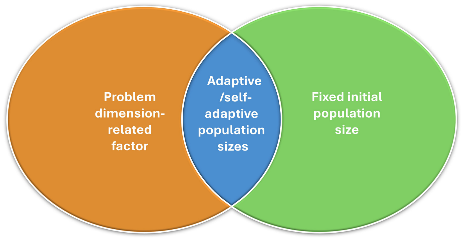
Since the inception of the DE algorithm, conventional guidelines have been proposed to provide users with recommendations for determining the population size. These guidelines suggest the selection of the population size either as a function of the problem dimension or the adoption of a fixed value as clearly highlighted in previous review studies [16]. Conventional guidelines suggesting population sizes based on problem dimensions often stem from limited experimental investigations, which may not be generalizable. Concrete evidence about a linear relationship between the population size and the problem dimensionality has never been found [17,18]. The study by Piotrowski in 2020 reveals a nonlinear relationship between the population size and the problem dimension in the context of the particle swarm optimization (PSO) algorithm [18]. There appears to be a lack of comprehensive research in the literature related to the DE algorithm that investigates the link between population size and problem-specific characteristics across various dimensions and complexities. Nevertheless, the practice of the adoption of a fixed value for the population size, based on experimental analysis, seems primarily applicable to the specific problems investigated. Determining the appropriate population size within the DE algorithm remains a daunting task, critically influencing DE performance.

Acknowledging the significance of the population size on the performance of the DE algorithm, researchers have increasingly explored adaptive DE strategies that provide more flexible and dynamic approaches. Accordingly, a plethora of research has emerged to address the challenge of improving DE performance by incorporating adaptive mechanisms to adjust the population size throughout the search process [19,20,21,22,23,24,25,26,27,28,29,30,31,32,33,34,35,36,37,38,39,40,41,42,43,44,45,46,47,48,49,50].

Numerous adaptive strategies have focused on reducing the population size throughout generations to enhance the DE search abilities and to achieve better convergence while reducing the computational burden [19,20,21,22,23,24,25,26,27]. Another perspective is the adoption of variable population size strategies, wherein the population size is dynamically varied based on certain information gathered during the optimization process, such as the achieved performance level, convergence speed, and problem-specific information [28,29,30,31,32,33,34,35,36,37,38,39,40,41]. In addition to the aforementioned strategies, self-adaptive population size strategies have also been proposed [42,43,44,45,46,47,48,49,50].

It is, however, worth mentioning that a significant number of studies, including those focused on adaptive DE strategies, have adopted the practice of determining the initial population either as a function of the problem dimension [27,28,34,37,38,40,41,43,44,47,48,50,51,52,53,54,55,56,57,58,59,60,61], or a fixed value [19,20,21,22,23,24,25,26,29,30,32,35,36,39,42,46,49,62,63,64,65,66,67,68,69,70,71]. Moreover, while dynamic population size adjustment offers a certain level of flexibility, setting a fixed initial population size may impose limitations of a predetermined population and could potentially restrict the ability of the algorithm to effectively respond to the dynamic nature of the search process. This limitation also arises in adaptive strategies that impose lower and upper limits for the population size, thereby becoming constrained by these bounds [16]. Piotrowski [16] emphasizes that the performance of self-adaptive strategies with lower and upper limits for the population size depends largely on these bounds. In a study by Zhu et al. [31], the population size increased beyond the upper bounds when the population stagnated.

Notably, the emergence of adaptive population size strategies did not resolve the problem of initial population size selection since the user is not relieved from the hassle of the determination of the initial populations. Furthermore, the adaptive strategies for the population size in the DE algorithm often introduce additional control parameters, and thus are difficult to implement and tune [72].

Despite the acknowledged significance of $N_P$, the guidelines for its determination exhibit a notable lack of clarity and precision, making it an ongoing research question that necessitates further investigation and refinement. The available guidelines for the determination of the population size in the DE algorithm have led to a one-size-fits-all setting that may not always align with the optimal parameters selection for specific problems. Such guidelines, although being widely applied, often fall short of accommodating the dynamic nature of different optimization scenarios, including the problem-specific characteristics and interrelationship between DE control parameters. A thorough examination of the presented papers reveals that the majority of studies focus on the adaptation of F and $CR$ together while adapting the population size individually [72]. The interaction between the population size and other DE control parameters is under-researched. Specifically, the side-effects introduced by individually changing the values of one control parameter on other DE control parameters have yet to be explored.

In light of the aforementioned challenges, the main objectives of this study are as follows:

• Evaluate the credibility and effectiveness of existing guidelines for setting the population size in the DE algorithm: Critically assess the efficacy of proposed guidelines for determining population size within the DE algorithm, considering various problem modalities and dimensional complexities.
• Investigate the correlations between population size and the fitness landscape characteristics of various problems: Analyze how varying population sizes affect DE performance across the distinct fitness landscapes of unimodal problems, multimodal problems, hybrid problems, and composition problems.
• Analyze the significance of the population size in the DE algorithm: Utilize functional analysis of variance (fANOVA) to quantitatively assess the relative importance of the population size ($N_P$), along with other DE control parameters, namely, the scale factor (F) and the crossover rate ($CR$).
• Investigate the interrelationship between the population size and other DE control parameters: Examine the interplay and dependencies between the population size ($N_P$) and other DE control parameters (F and $CR$) using fANOVA. More specifically, the objective is to capture any possible interaction between DE control parameters and to uncover how these parameters collectively affect the performance of the DE algorithm.

It is worth mentioning that this study employs the original differential evolution algorithm as proposed by Storn and Price [9]. The selection of the original DE algorithm allows for a focused investigation without the confounding effects of advanced DE variants. Since the guidelines for determining the population size proposed in past studies are based on the original DE, this paper continues to investigate the credibility of these guidelines specifically within the context of the original DE algorithm. This investigation is necessary to facilitate a comprehensive understanding of the credibility of these guidelines, providing a performance reference for potential future studies involving advanced DE variants. Concerning DE, research that considers various problem modalities, the relative importance, and the interactions between DE control parameters has yet to be reported in the relevant literature.

To effectively address the research objectives, this paper is organized as follows: Section 2 offers a detailed exploration of the necessary background information and delivers a review of the existing literature relevant to the topic. Section 3 provides an overview of the basic DE algorithm considered in this study, along with the statistical approach employed, namely, the functional analysis of variance fANOVA. The methodology, experimental analysis, and the results and discussion are presented in Section 4, Section 5, Section 6, Section 7 and Section 8. Finally, Section 9 summarizes the key findings of the research and highlights areas for possible future directions.

2. Background and Related Work

The population size within the DE algorithm constitutes a critical control parameter that significantly affects the performance of the algorithm. The judicious selection of appropriate population size plays a crucial role in striking a balanced exploration-exploitation process and influencing the convergence rate of the DE algorithm. In the context of the DE algorithm, the population size has been set either as a problem dimension-related factor or as a fixed value. This section covers the related literature on both aspects, followed by a detailed background on adaptive population sizes and the challenges in selecting the initial population size in the DE algorithm.

2.1. Population Size as a Problem Dimension-Related Factor

In their original research published in 1997, Storn and Price articulated that effective tuning of the DE control parameters to achieve desirable outcomes is not a tedious task and recommended the adoption of a population size ranging from $5\times D$ to $10\times D$ (where D is the problem dimension) [9]. Subsequently, in 1999, Storn and Price further proposed enlarging the population size to avoid premature convergence, advocating for a population size of $20\times D$ [73]. Thus, a general perception of setting the population size as a dimensionality-dependent parameter has been widely acknowledged and applied [74]. As a result, a population size that is equal to $10\times D$ has been frequently used [75,76,77,78,79,80,81].

The general guidelines provided by Storn and Price regarding the determination of population size in the DE algorithm have been argued in various studies. Particularly, several studies have highlighted that the selection of appropriate values for the population size in the DE algorithm is more challenging than expected [82]. Gämperle et al. [74] mentioned that the guidelines provided by Storn and Price lack generality and are, therefore, unsuitable for practical applications. Instead, Gämperle et al. suggested employing population sizes ranging from $3\times D$ and $8\times D$. Nevertheless, the conclusions drawn by Gämperle et al. were based on limited experimental studies that focused on two unimodal and two multimodal problems. Additionally, several studies have indicated that a population size lower than or equal to the dimensionality of the problem could be advantageous in specific instances [17,83,84]. Figure 1 provides a visual summary of population size setting strategies within the DE algorithm, illustrating fixed-value, problem dimension-related, and adaptive/self-adaptive population size approaches.

Chen et al. [17] critiqued the practice of linearly increasing the population size as the problem dimension increases, referring to the principle of the “curse of dimensionality”. The challenge posed by the curse of dimensionality was first demonstrated by Bellman in 1957 [85], revealing that the search space volume grows exponentially with increased problem dimensionality in continuous domains. Chen et al. [17] argued that despite the well-known effects of the curse of dimensionality, the population sizes employed to explore higher dimensional problems usually grow only linearly and further concluded that employing a population size smaller than the problem dimension had a detrimental impact on DE convergence and resulted in the algorithm becoming trapped within a subspace of the overall search space. However, it is worth noting that the experimentation conducted by Chen et al. was based solely on the unimodal spherical problem, indicating a possible limitation in generalizing their conclusions. Notably, the conventional guidelines that suggest setting the population size to be linearly proportional to the problem dimension have never been justified, and empirical evidence to establish a solid linear correlation between population size and problem dimensionality has never been reported. Piotrowski et al. [18] identified a nonlinear logarithmic relationship between population size and problem dimension within the context of the PSO algorithm based on experimental studies.

2.2. Population Size as a Fixed Value

Besides setting the population size as a dimensionality-related factor, numerous studies on DE have employed a fixed value for the population size [82], irrespective of problem dimensionality or any other problem characteristics. For instance, studies have used 10 individuals [86], 20 individuals [87], 30 individuals [88], 50 individuals [6], 60 individuals [89,90], 75 individuals [91], 100 individuals [20], 200 individuals [92], and 250 individuals [93]. The selection of a fixed population size has been typically applied based on trial-and-error strategies. Such strategies are subjective and have rarely been justified. The general guidelines to set the population size either as a problem dimensionality-related factor or a fixed value imply that the user has previous knowledge about the problem being considered, although such knowledge is scarcely available.

2.3. Adaptive and Self-Adaptive Population Size Approaches

Recognizing the paramount importance of the population size, a considerable volume of research has proposed diverse strategies aimed at adapting the population size within the DE algorithm. Today, there exists a plethora of strategies to dynamically adjust the population size during the search process. Although the significance of adaptive population sizing strategies is fully acknowledged, it is important to note that these strategies did not resolve the problem of population size setting. Specifically, the adaptive strategies have not eliminated the necessity for users to select an initial population size or to define limits for population size adjustment. Hence, determining the optimal population size that addresses each unique problem scenario remains an area of ongoing research. Aspects such as the adaptation of the population size considering problem-specific characteristics and the interrelationships between DE control parameters are still pertinent and unexplored.

2.4. Challenges in Selecting the Initial Population Size in DE

It is of utmost importance to highlight that the adaptive population size strategies within the DE algorithm still rely on the utilization of initial populations either as a problem dimension-related factor or a predetermined fixed value. Brest et al. [47], who proposed a novel self-adaptive DE variant, mentioned that “Recently, some works are related to changing population size during the optimization process, but there are still no general guidelines how to set the population size at the beginning of the optimization process, when to change (question if to increase or decrease remains open, too), etc. Since all parameters are related to each other and they are depending on the optimization problem being solved, further works are necessary". Zhang et al. [57] wrote that “the relationship between population size and the problem dimension still remains to be deeply studied, while for the third type, the simple ignorance of all characteristics of a specific problem may result in ineffectiveness". However, the initial population size in Zhang et al. [57] was selected as a function of the problem dimension, as they wrote “in this paper, the population size varies in a given range, and the upper and lower bounds of the population size are initialized as $10\times D$ and D, respectively, while the initial population size $P{S}_{init}$ is set at 100, and these settings have referred to some conclusions in Piotrowski [16]".

In 2017, Piotrowski published a comprehensive and informative review [16] that thoroughly investigated the nuances of the DE population size as a crucial control parameter. The review not only shed light on previously unexplored research areas surrounding the population size, but also emphasized the pressing need for further investigation to optimize the DE population size. Areas such as considering problem-specific characteristics when setting the DE population size, the relative importance of $N_P$, F, and $CR$, and the interrelationship between DE control parameters were overlooked in [16].

Furthermore, several applications have yielded evidence that some control parameters tend to be more critical than others [94,95]. This is further corroborated by research investigating the relative importance of control parameters in the particle swarm optimization (PSO) algorithm applying the functional analysis of variance (fANOVA) [96]. However, research on the relative importance and interrelationships of DE control parameters using fANOVA has never been reported in the existing literature.

Additionally, a clue into the interaction between DE control parameters was reported in [97], where the overall optimization and the relationship between DE control parameters were investigated. The findings in [97] demonstrated a close correlation between DE control parameters, and the optimal population sizes were observed to range between 30 and 40 individuals [97]. However, the results in [97] were specifically derived from experiments conducted on the unmanned aerial vehicle (UAV) path planning problem.

Further research concerning the population size within the DE algorithm was reported by Alić et al. [98] who analyzed the effect of population size on the performance of the DE algorithm and proposed an adaptive DE variant. The adaptive DE proposed in [98] utilized a population re-setting strategy, in which the population is reinitialized upon reaching a certain threshold of population diversity, and concluded that further increment of the population size detrimentally affects the overall performance of the DE algorithm. However, the study in [98] omits key information, such as the correlation between the population size and the problem dimension, the interrelationships between DE control parameters, and the link between problem-specific characteristics and the DE population size. These omissions highlight significant gaps in the existing literature and underscore the necessity for comprehensive analysis to address these gaps and enhance the performance of the DE algorithm.

Moreover, in a recent review based on the state-of-the-art works published in 2022 [99] adaptive adjustment of DE control parameters, based on population diversity and fitness landscape characteristics, is proposed as potential future work. The analysis in this paper aims to contribute to this promising future direction by investigating the impact of the existing guidelines to determine the population size on DE performance concerning problem characteristics and the interaction between DE control parameters, where such interaction should be used to devise more efficient adaptive DE variants.

Hutter et al. [100] introduced a novel statistical approach termed the functional analysis of variance (fANOVA), which is a powerful statistical tool used to quantify the importance of each control parameter individually and to provide insights into the interactions between control parameters [100]. The utility of fANOVA extends across various domains, and was therefore used to provide valuable insights into the importance of control parameters and their interactions in neural networks [101,102,103,104] and machine learning [105,106]. In the context of swarm-based algorithms, the fANOVA approach was used to quantify the importance of control parameters for the particle swarm optimization (PSO) algorithm [96] and the multi-guide PSO [107]. In this paper, fANOVA is used to quantify the importance of the population size and to investigate the interaction between $N_P$ and the other DE control parameters, namely, F and $CR$.

By carefully examining the ideas presented in the above-mentioned studies, it becomes evident that further research into optimal population sizes remains imperative to gain a comprehensive understanding of how to set the population size according to the specific characteristics of optimization problems and the interrelationships between DE control parameters. All the discussions above have cultivated and sustained the motivation for this research.

3. Differential Evolution

This section introduces the basic differential evolution algorithm as employed in this study. Differential evolution is an efficient population-based optimization algorithm proposed by Storn and Price for solving global optimization problems over continuous domains [9]. Similar to the majority of EAs, DE utilizes a population consisting of D dimensional vectors as a population for each generation. Starting with a random initial population, DE utilizes three evolutionary operators, namely, mutation, crossover, and selection to generate new candidate solutions. The operators are iteratively applied to each individual (parent) in the population to generate offspring. Afterwards, the parent is compared to its respective offspring, and the fitter individual is selected to participate in the next generation. The following is a brief description of the DE operators.

3.1. Mutation

The mutation operator creates a mutant vector for each individual in the current population by adding a weighted differential to a target vector. Specifically, for each parent, ${\mathbf{x}}_i\left(t\right)$ , a mutant vector, ${\mathbf{u}}_i\left(t\right)$, is generated by selecting a target vector, ${\mathbf{x}}_{i_1}\left(t\right)$, from the population, such that $i\ne$$i_1$. Then, two individuals, ${\mathbf{x}}_{i_2}\left(t\right)$ and ${\mathbf{x}}_{i_3}\left(t\right)$, are randomly selected from the population such that $i\ne i_1\ne i_2\ne i_3$ and $i_1$, $i_2$, $i_3$∼ U(1, $N_P$). The mutant vector is generated as follows [9]:

$${\mathbf{u}}_i\left(t\right)={\mathbf{x}}_{i_1}\left(t\right)+F\ast ({\mathbf{x}}_{i_2}\left(t\right)-{\mathbf{x}}_{i_3}\left(t\right))$$

(1)

where F$\in (0,\infty )$ is the scale factor that controls the amplification of the differential variation, $({\mathbf{x}}_{i_2}\left(t\right)-{\mathbf{x}}_{i_3}\left(t\right))$.

3.2. Crossover

The crossover operator recombines components of the parent vector, ${\mathbf{x}}_i\left(t\right)$, and the mutant vector, ${\mathbf{u}}_i\left(t\right)$, to generate a trial vector, ${\mathbf{x}}_i^{\prime }\left(t\right)$, as follows:

$$x_{ij}^{\prime }\left(t\right)=\left\{\begin{array}{cc}{u}_{ij}\left(t\right)\hfill & \mathrm{if}(r\le \mathrm{CR}\left|\right|j=j_{rand})\hfill \\ x_{ij}\left(t\right)\hfill & \mathrm{otherwise}\hfill \end{array}\right.$$

(2)

where $x_{ij}\left(t\right)$ refers to the $j^{th}$ element of the vector ${\mathbf{x}}_i\left(t\right)$ and r is a random value sampled from a uniform distribution over $(0,1)$. The crossover points are randomly selected from the set of possible crossover points, $\{1,2,\dots ,D\}$.

3.3. Selection

Participation in the next generation depends on the applied selection scheme. The basic DE algorithm applies a greedy selection scheme, where the trial vector, ${\mathbf{x}}_i^{\prime }\left(t\right)$, is compared to the parent vector, ${\mathbf{x}}_i\left(t\right)$, and the vector which yields a better fitness value (i.e., a smaller cost function value for a minimization problem) survives into the next generation.

3.4. Basic Differential Evolution

Several DE variations have been proposed in the literature. The notation DE/x/y/z is used to define specific DE strategies. In this notation, x is the method of selecting the target vector, y indicates the number of difference vectors used, and z indicates the crossover method used. The basic DE/rand/1/bin is used in this paper, where the target vector is randomly selected, one difference vector is used in the mutation operation, and binomial crossover is used. The DE/rand/1/bin strategy is summarized in Algorithm 1.

Algorithm 1 Differential Evolution DE/rand/1/bin

1: Set the generation counter, t = 0; 2: Initialize the control parameters, $N_P$, F and $CR$; 3: Initialize the population, $G\left(0\right)$, of $N_P$ individuals; 4: while stopping condition(s) not true do 5:     for each individual, ${\mathbf{x}}_i\left(t\right)\in G\left(t\right)$ do 6:         Evaluate the fitness, $f\left({\mathbf{x}}_i\left(t\right)\right)$; 7:         Select three random integers $i_1$, $i_2$, $i_3$, ∈ {1,..., $N_P$} such that i≠$i_1$≠$i_2$≠$i_3$ 8:         Select a random integer $j_{rand}\in \{1,2,\cdots ,D\}$ 9:         for each parameter j do 10:            $x_{ij}^{\prime }\left(t\right)=\left\{\begin{array}{cc}{u}_{ij}\left(t\right)\hfill & \mathrm{if}\left(rand\right(0,1)\le CR\left|\right|j=j_{rand})\hfill \\ x_{ij}\left(t\right)& \mathrm{otherwise}\hfill \end{array}\right.$ 11:         end for 12:         if $f\left({\mathbf{x}}_i^{\prime }\left(t\right)\right)$ is better than $f\left({\mathbf{x}}_i\left(t\right)\right)$ then 13:            Add ${\mathbf{x}}_i^{\prime }\left(t\right)$ to $G(t+1)$; 14:         end if 15:         else 16:         Add $\left({\mathbf{x}}_i\left(t\right)\right)$ to $G(t+1)$; 17:     end for 18:     $G\left(t\right)=G(t+1)$; 19: end while 20: Return the individual with the best fitness as the solution;

3.5. Functional Analysis of Variance

The functional analysis of variance (fANOVA) [100] is a powerful statistical technique used to decompose the observed variation in a response function into additive components associated with each subset of its input variables. The decomposition of variance in the response is used to analyze the extent to which performance variability is caused by a single control parameter or combinations of control parameters. The mathematical formulation for fANOVA is outlined below: Given an algorithm A that has n control parameters with domains ${\Theta }_1,\dots ,{\Theta }_n$ and configuration space $\Theta ={\Theta }_1\times \cdots \times {\Theta }_n$. Let

• the control parameters set be $N=\{1,\dots ,n\}$;
• a control parameters instantiation be denoted as $\theta =\langle {\theta }_1,\dots ,{\theta }_n\rangle$ with ${\theta }_i\in {\Theta }_i$;
• a control parameters subset be denoted as $\Phi =\{{\varphi }_i,\dots ,{\varphi }_j\}$, and the associated partial parameters instantiation is given ${\theta }_{\Phi }=\langle {\theta }_{\varphi i},\dots ,{\theta }_{\varphi j}\rangle$ with a subset $\Phi \subseteq N$;
• $X\left({\theta }_{\Phi }\right)$ be the extension set of ${\theta }_{\Phi }$, defined as the set of control parameters configurations that form a complete instantiation when combined with ${\theta }_{\Phi }$, denoted by ${\theta }_T$ where $T=N\setminus \Phi$;
• the performance metric to quantify the performance of A denoted by $m({\theta }_i,{\pi }_j)$ over a set of k problems, ${\pi }_1,\dots ,{\pi }_k$.

Then, the marginal performance of ${\theta }_{\Phi }$, denoted as $\widehat{m}$, is defined as the expected variance in performance associated with ${\theta }_{\Phi }$ with respect to all instantiations of the remaining control parameters T, given by

$$\widehat{m}\left({`}_{\Phi }\right)={\displaystyle \frac{1}{\left|\right|{\Theta }_T\left|\right|}}\int \widehat{y}\left({\theta }_T\right)d{\theta }_T,$$

(3)

where $\widehat{y}$ : $\mapsto \mathbb{R}$, and $\left|\right|{\Theta }_T\left|\right|={\prod }_{i=1}^k\left|\right|{\Theta }_T\left|\right|$. In short, given a subset $\Phi \subset N$, $\widehat{m}(\theta \Phi )$ provides an estimation of the average performance across all instantiations in the parameter space $N\setminus \Phi$ when the parameters of $\Phi$ are fixed at ${\theta }_{\Phi }$.

The basic concept of the prediction technique in the context of fANOVA involves the construction of a random forest, where each regression tree defines a partition of the configuration space $\Theta$, such that the marginal prediction of the entire forest is obtained by averaging the prediction over each tree [100].

The fANOVA approach uses the predicted marginal performance $\widehat{m}$ to decompose the observed variation of a response value $\mathbb{V}$ into additive components associated with each subset of its input variables $\Phi \subset N$ as follows:

$$\mathbb{V}=\sum _{\Phi \subset N}{\mathbb{V}}_{\Phi },$$

(4)

where ${\mathbb{V}}_{\Phi }$ is the contribution of subset $\Phi$ to the total variance. The importance of each subset can be computed as the fraction of the variance of the subset associated with the total performance variance. A larger fraction of variance associated with a particular control parameter indicates a higher sensitivity to the values of that control parameter. Therefore, control parameters with higher values for the variance are more influential and thus should have a higher priority when tuning control parameter values.

4. Empirical Analysis

This section presents the empirical analysis of two carefully designed experiments conducted to achieve the primary objectives outlined in Section 1. The experimental setup is elaborated upon in detail in Section 5, providing a comprehensive account of the research methodology employed. Subsequently, Experiment 1, entitled “Analyzing the Impact of Population Size on DE Performance Across Various Problem Modalities and Dimensional Complexities”, is presented in Section 6. This experiment seeks to assess the guidelines currently employed to determine the population size and investigates the influence of population size on the performance of the DE algorithm across a range of problem modalities and dimensional complexities. It specifically aims to address Objectives 1 and 2. Following this, Experiment 2, titled “The Importance of Population Size and its Interrelation with Other DE Control Parameters”, is discussed in Section 7. This experiment focuses on the significance of population size and its interrelationship with other control parameters within the DE algorithm, targeting Objectives 3 and 4.

5. Experimental Setup

To achieve the objectives, the DE/rand/1/bin strategy was applied to a set of well-known benchmark problems. Since population size determination guidelines have been derived from the original DE, this paper continues to focus on the original DE to analyze the credibility of these guidelines. Also, the CEC provides predefined benchmark suites that are commonly used to test algorithm performance [108,109,110,111]. The standard problems defined in CEC 2014 [109] were chosen for the purpose of experimentation. The selection of the CEC 2014 benchmark suite is primarily attributed to its ability to provide a diverse set of problems that cover a wide range of characteristics, complexities, and dimensions. Despite being over ten years old, the CEC 2014 problems remain widely used due to their diversity and complexity, which continue to benchmark modern algorithms, including advanced variants of the DE algorithm. Moreover, these benchmark problems have been extensively used to provide a consistent testbed for analyzing the population size for DE [16] and other well-known algorithms, like the PSO algorithms recently in 2020 [18], which enables comparisons with previous studies and build upon the existing literature. (The following study demonstrates that there are no significant differences in the fitness landscape characteristics between the CEC 2014 benchmark functions and those in later benchmark sets. Therefore, CEC 2014 remains a sufficient and relevant benchmark suite [112]).

The CEC 2014 benchmark suite comprises 30 problems and covers relatively simple unimodal problems (problems 1–3), multimodal problems (problems 4–16), hybrid problems (problems 17–22), and other composition problems (problems 23–30, which are considered extremely complex). All problems are scalable, which were tested using 10, 20, 30, 50, and 100 dimensions. Detailed descriptions of these problems are given in the work by Liang et al. [110]. The CEC 2014 benchmark problems are sufficient to provide evidence supporting the main hypothesis and to draw sound conclusions on the aspects investigated in this study.

For each problem, the maximum number of function evaluations was $10,000\times D$ (where D is the problem dimension), as previously advised in Liang et al. [109]. Consequently, simulations using 20 individuals were run for 5000 iterations, whereas simulations using 100 individuals were run for 1000 iterations. Moreover, as per the recommendations in [109], a total of 51 independent runs were performed for each problem, per dimension, and parameter setting combination. The obtained results were subjected to rigorous statistical validation, as detailed in the subsequent sections.

Two distinct experiments were conducted to achieve the objectives of this paper. The first experiment focuses on assessing the credibility of the proposed guideline used to determine the population size in the DE algorithm and empirically investigates how varying the population size affects DE performance across various fitness landscapes associated with different problem modalities. In this experiment, the population size was the sole control parameter that was varied using a range of values. The other control parameters of DE, i.e., the scale factor F and the crossover rate $CR$, were maintained at constant values in accordance with the recommendations by Storn and Price in [9]. The analysis is conducted for each problem at various specified dimensions. Keeping all other control parameters fixed while changing the population size for diverse problem modalities and various problem dimensions allowed for a comprehensive assessment of the proposed population size guidelines on the performance of the DE algorithm and the effect of various population sizes on problem modalities.

In the second experiment, the values of all DE control parameters, including the population size, the crossover rate, and the scale factor, were systematically varied. This was done to achieve the objective of examining the relative importance of the population size and the mutual interactions between DE control parameters using the fANOVA technique. A comprehensive discussion of the experimental procedures and results obtained from both experiments is provided in the following sections, alongside detailed insights and analysis.

6. Experiment 1: Analyzing the Impact of Population Size on DE Performance Across Various Problem Modalities and Dimensional Complexities

This experiment investigates the effect of population size on DE performance, beginning with evaluating the impact of population size and the credibility of existing guidelines in Section 6.1, followed by an exploration of its relationship with various problem classes in Section 6.2, and concluding with a statistical analysis and comprehensive discussion of the findings in Section 6.3.

6.1. Evaluating Population Size Impact and Credibility of Existing Guidelines

For the purposes of this experiment, a range of population sizes consisting of 10, 20, 30, 40, 50, 70, 100, 200, 300, 400, 500, 700, and 1000 individuals were utilized. The scale factor F and the crossover rate $CR$ were set at 0.5 and 0.9, respectively, as suggested in [9]. For each benchmark problem, and for each dimension, the overall average fitness of the best solutions found over 51 independent runs was reported, along with the corresponding standard deviation. Notably, a lower average fitness value indicates a better solution. The performance assessment relied on the quality of the solutions obtained at the termination of the algorithm. Based on solution quality, the population sizes were ranked from best to worst. Thus, the population size that achieved the highest quality was assigned the topmost rank of 1, whereas the population size associated with the lowest quality was assigned a rank of 13. The average rank of every population size for each problem per dimension was reported. Furthermore, in order to evaluate the performance of each population size across all problems within a specific problem dimension, the mean average rank was calculated. The mean average rank represents the performance of a particular population size across all 30 problems per a specific dimension. The lower the mean average rank, the better the performance.

Statistical tests were conducted to validate the hypothesis of whether the average ranks achieved with various population sizes were statistically significant. Accordingly, the statistical significance of the multiple comparisons among all population sizes for every problem per dimension was examined by means of the Friedman test followed by the post hoc Shaffer static procedure as suggested in Derrac et al. [113]. The tests were carried out at an $\alpha =$ 0.05 significance level. A graphical illustration of the mean average ranks with respect to different population sizes and various dimensions for all problems is given in Figure 2.

Figure 2 illustrates that for all dimensions, the mean average ranks were relatively high for small population sizes (i.e., $N_P$ = 10). This high rank indicates a worsened performance. However, as the population size increased to a moderate value, the performance exhibited the best levels. Subsequently, the performance continued to improve only up to a specific limit, beyond which the performance gradually deteriorated again to reach its worst levels with extremely large population sizes (as can be observed for D = 10, D = 30, and D = 50). This observation is in accordance with the research conducted by Malan and Engelbrecht [15]. An exception was for D = 100, where population sizes beyond $N_P$ = 30 did not significantly affect performance. Generally, a population size within the range of 20 to 30 was found to be the most appropriate across all dimensions.

6.2. Population Size in Relation to Problem Classes in DE

To further investigate the correlations between population size and the fitness landscape of various problems (utilizing problem modality as the key characteristic of varied fitness landscapes), the mean average ranks were calculated for each population size across the unimodal, multimodal, hybrid, and composition problems in dimensions D = 10, D = 30, D = 50, and D = 100, as shown in Figure 3. A deeper understanding of the relationship between population size, problem modalities, and DE performance can be obtained by examining the mean average ranks.

The trends observed in Figure 2 were further supported by the results presented in Figure 3. Similar trends were apparent for the unimodal, multimodal, and hybrid problems, as illustrated in Figure 3a, Figure 3b, and Figure 3c, respectively. It is evident from Figure 3a–c, that small population sizes are associated with high overall average ranks, indicating poorer performance. Conversely, larger population sizes improved the performance up to a certain threshold level, beyond which the performance either remained steady or even deteriorated.

However, some exceptional observations were evident in the case of the multimodal problems with D = 100, as depicted in Figure 3b; specifically, increasing the population size beyond $N_P$ = 30 did not lead to noticeable performance enhancements. Moreover, it was observed for the composition problems across all dimensions that the performance improved as the population size increased, as shown in Figure 3d. Notably, larger population sizes yielded better results for the composition problems. This investigation uncovers a unique observation not previously emphasized in the DE literature that larger population sizes benefit particular optimization problems, specifically, the composition problems. Thus, the findings resonate with the second objective of this paper and provide solid evidence about the relationship between problem characteristics and optimal population sizes. It is worth noting that the search space for the composition problems is more complex compared to the unimodal problems, multimodal problems, and hybrid problems. More detailed information and plots regarding the CEC 2014 problems are available in [109,112].

As mentioned earlier, the Friedman–Shaffer statistical test was performed to verify the statistical significance of the results. For each problem per dimension and with 13 population sizes, a total of $m=78$ comparisons were performed $(m=K\times (K-1)/2)$, where K is the number of population sizes chosen for the experiment (i.e., 13). Therefore, a total of 9360 pair-wise comparisons were conducted throughout the experiment.

It is important to note that the Friedman test calculates the average ranks of the population sizes and specifies whether these average ranks are statistically significantly different at $\alpha =0.05$. In the case of multiple comparisons among all population sizes, the Shaffer procedure is needed to verify the significance of all possible pair-wise comparisons and to control the accumulated family pair-wise error rate (denoted as FWER and defined as the probability of making one or more false discoveries among all the hypotheses when performing multiple pair-wise tests). Accordingly, the statistical results in this research are interpreted as follows: considering all statistically significant pair-wise comparisons provided by the Shaffer post hoc procedure, the total number of wins is calculated for each population size. A win indicates that a particular population size performed significantly better (having a lower average rank compared to that of its competitor, and the test shows a statistically significant difference). Similarly, losses are counted for all population sizes. In cases where two or more population sizes performed equally, ties are recorded. Ties were rewarded equally, and wins were credited for all tied population sizes.

6.3. Statistical Analysis and Extended Discussion on Population Size Implications

To simplify and consolidate the results of the statistical analysis into a single performance measure, a metric referred to as the ‘score’ is applied. The score for each population size is computed as the difference between the total number of wins and losses. A higher score indicates better statistically significant performance associated with a specific population size. The statistical results, represented by the scores, are summarized in

Table A1. Results of the statistical analysis represented by score for all CEC 2014 problems in dimension $D=10$.

Function Class	Functions	${\mathit{N}}_{\mathit{P}}$ Values
		10	20	30	40	50	70	100	200	300	400	500	700	1000
Unimodal	F1	−4	10	9	8	6	4	2	−1	−3	−6	−5	−9	−11
	F2	−8	7	7	7	7	7	7	−1	−3	−6	−7	−8	−9
	F3	−8	5	6	6	6	6	6	6	$-4$	−5	−6	−9	−9
Multimodal	F4	−5	−5	7	0	−5	5	5	6	5	1	−2	−5	−7
	F5	7	5	6	4	5	−1	2	4	−7	−7	−4	−6	−8
	F6	4	5	5	5	5	5	5	5	−5	−7	−8	−9	−10
	F7	5	10	7	5	7	4	0	−2	−4	−5	−9	−8	−10
	F8	−2	−5	−5	2	0	5	0	−2	0	5	2	2	−2
	F9	11	10	6	5	5	4	−2	−5	−7	−5	−5	−7	−10
	F10	1	8	8	8	8	6	1	−2	−6	−6	−8	−8	−10
	F11	11	8	6	6	4	5	0	−5	−5	−7	−7	−7	−9
	F12	9	9	7	7	0	−2	−4	−4	−4	−4	−5	−4	−5
	F13	0	0	0	0	0	0	0	0	0	0	0	0	0
	F14	0	0	0	0	0	0	0	0	0	0	0	0	0
	F15	10	4	2	4	2	0	1	0	0	−2	−5	−6	−10
	F16	8	8	7	6	6	3	4	−7	−7	−7	−7	−7	−7
Hybrid	F17	−6	7	9	8	8	5	3	1	−4	−6	−7	−8	−10
	F18	−8	9	9	8	7	5	2	−1	−2	−5	−7	−8	−9
	F19	−1	7	7	7	7	7	6	−3	−3	−7	−9	−9	−9
	F20	−8	7	8	8	8	7	3	−1	−3	−4	−7	−9	−9
	F21	−8	8	8	8	8	7	1	0	−2	−6	−6	−8	−10
	F22	−7	6	6	7	7	7	7	1	−4	−6	−7	−8	−9
Composition	F23	−10	1	2	2	2	2	2	2	2	2	2	2	−11
	F24	7	9	8	7	5	3	1	−1	−7	−8	−8	−8	−8
	F25	−5	5	5	5	5	3	2	0	0	−4	−6	−4	−6
	F26	0	0	0	0	0	0	0	0	0	0	0	0	0
	F27	−2	0	0	0	0	0	0	0	0	0	1	0	1
	F28	−6	0	−2	0	−2	0	1	0	3	1	3	1	1
	F29	−2	0	0	0	0	0	1	0	0	0	1	0	0
	F30	0	0	0	0	0	0	0	0	0	0	0	0	0
Overall Total		−17	138	138	133	111	97	56	−10	−70	−104	−126	−150	−196
Overall Unimodal		−20	22	22	21	19	17	15	4	−10	−17	−18	−26	−29
Overall Multimodal		59	57	56	52	37	34	12	−12	−40	−44	−58	−65	−88
Overall Hybrid		−38	44	47	46	45	38	22	−3	−18	−34	−43	−50	−56
Overall Composition		−18	15	13	14	10	8	7	1	−2	−9	−7	−9	−23

,

Table A2. Results of the statistical analysis represented by score for all CEC 2014 problems in dimension $D=30$.

Function Class	Functions	${\mathit{N}}_{\mathit{P}}$ Values
		10	20	30	40	50	70	100	200	300	400	500	700	1000
Unimodal	F1	7	8	7	6	6	4	1	−3	−5	−7	−7	−8	−9
	F2	−10	7	7	7	7	7	7	−2	−3	−4	−6	−8	−9
	F3	−9	7	7	7	7	7	7	−2	−3	−4	−6	−8	−10
Multimodal	F4	−8	7	9	8	8	5	2	0	−2	−5	−6	−8	−10
	F5	1	0	0	0	0	0	0	0	0	0	−1	0	0
	F6	4	7	9	8	7	5	1	−3	−5	−7	−8	−9	−9
	F7	−10	1	−2	1	1	1	0	1	1	1	1	2	2
	F8	9	10	8	6	4	3	1	−4	−6	−7	−7	−8	−9
	F9	11	7	5	5	5	5	3	−4	−6	−7	−7	−8	−9
	F10	9	9	8	6	4	2	1	−3	−5	−7	−7	−8	−9
	F11	9	7	6	6	4	3	1	−4	−5	−7	−6	−7	−7
	F12	0	0	0	0	0	0	0	0	0	0	0	0	0
	F13	0	0	0	0	0	0	0	0	0	0	0	0	0
	F14	0	0	0	0	0	0	0	0	0	0	0	0	0
	F15	−2	9	7	7	7	4	4	−2	−4	−4	−5	−10	−11
	F16	9	6	5	5	4	4	1	−1	−6	−6	−6	−8	−7
Hybrid	F17	8	9	8	7	5	3	1	−4	−6	−6	−7	−8	−10
	F18	2	8	9	8	7	5	1	−2	−5	−6	−8	−9	−10
	F19	−8	7	7	7	7	7	6	0	−3	−6	−7	−8	−9
	F20	−8	8	9	8	8	6	1	−1	−2	−5	−7	−8	−9
	F21	0	8	9	9	8	4	1	−2	−5	−7	−8	−8	−9
	F22	5	6	6	6	6	6	5	−2	−6	−7	−8	−8	−9
Composition	F23	−10	3	3	3	3	3	3	3	3	3	3	−10	−10
	F24	−10	−2	6	7	7	7	7	6	0	−3	−7	−9	−9
	F25	9	10	8	6	4	2	1	−2	−6	−7	−8	−8	−9
	F26	−8	−1	0	−3	0	1	1	1	1	2	1	2	3
	F27	−5	0	0	0	0	0	0	1	1	0	1	1	1
	F28	−8	−1	0	−2	1	0	1	1	1	3	1	2	1
	F29	−7	0	0	0	0	0	1	1	1	1	1	1	1
	F30	−8	−1	0	0	0	1	1	1	1	1	1	2	1
Overall Total		−28	139	141	128	120	95	59	−26	−74	−101	−123	−156	−174
Overall Unimodal		−12	22	21	20	20	18	15	−7	−11	−15	−19	−24	−28
Overall Multimodal		32	63	55	52	44	32	14	−20	−38	−49	−52	−64	−69
Overall Hybrid		−1	46	48	45	41	31	15	−11	−27	−37	−45	−49	−56
Overall Composition		−47	8	17	11	15	14	15	12	2	0	−7	−19	−21

,

Table A3. Results of the statistical analysis represented by score for all CEC 2014 problems in dimension $D=50$.

Function Class	Functions	${\mathit{N}}_{\mathit{P}}$ Values
		10	20	30	40	50	70	100	200	300	400	500	700	1000
Unimodal	F1	10	9	8	6	4	2	0	−2	−4	−7	−8	−9	−9
	F2	−10	6	6	6	6	6	6	6	−4	−5	−6	−8	−9
	F3	5	10	8	7	5	3	1	−2	−4	−7	−8	−9	−9
Multimodal	F4	−10	7	8	7	6	6	5	2	−3	−5	−5	−8	−10
	F5	0	0	0	0	0	0	0	0	0	0	0	0	0
	F6	1	8	8	8	8	6	1	−2	−5	−6	−8	−9	−10
	F7	−10	6	6	6	6	6	6	6	−4	−5	−6	−8	−9
	F8	10	9	7	6	4	3	0	−2	−4	−6	−8	−9	−10
	F9	10	9	7	5	4	3	2	−2	−6	−7	−8	−8	−9
	F10	10	9	8	6	4	2	1	−2	−6	−7	−8	−8	−9
	F11	0	0	0	0	0	0	0	0	0	0	0	0	0
	F12	0	0	0	0	0	0	0	0	0	0	0	0	0
	F13	6	8	7	7	6	4	0	−5	−6	−6	−7	−7	−7
	F14	0	0	0	0	0	0	0	0	0	0	0	0	0
	F15	−9	9	8	7	7	5	3	0	−2	−3	−6	−9	−10
	F16	12	−1	−1	−1	−1	−1	−1	−1	−1	−1	−1	−1	−1
Hybrid	F17	10	9	8	5	4	3	2	−4	−6	−6	−7	−8	−10
	F18	−8	7	7	7	7	7	6	−1	−3	−5	−7	−8	−9
	F19	−10	−1	8	8	8	8	7	1	−2	−4	−6	−8	−9
	F20	6	11	8	6	5	4	1	−3	−6	−7	−8	−8	−9
	F21	10	10	8	5	4	3	1	−5	−7	−7	−7	−7	−8
	F22	−11	−4	1	1	1	1	1	1	2	1	2	2	2
Composition	F23	−9	−3	1	0	−3	1	1	1	3	3	3	1	1
	F24	−8	−3	−3	1	0	0	1	3	1	1	3	1	3
	F25	0	0	0	0	0	0	0	0	0	0	0	0	0
	F26	−9	−6	−1	−3	1	2	1	4	2	2	3	1	3
	F27	−4	0	0	0	−1	1	0	0	1	2	0	0	1
	F28	−2	0	0	0	0	0	0	0	1	0	1	0	0
	F29	−10	−2	−1	1	1	1	1	1	1	3	1	1	2
	F30	−1	0	0	0	0	0	0	0	0	0	0	1	0
Overall Total		−21	107	116	101	86	76	46	−6	−62	−82	−101	−125	−135
Overall Unimodal		5	25	22	19	15	11	7	2	−12	−19	−22	−26	−27
Overall Multimodal		20	64	58	51	44	34	17	−6	−37	−46	−57	−67	−75
Overall Hybrid		−3	32	40	32	29	26	18	−11	−22	−28	−33	−37	−43
Overall Composition		−43	−14	−4	−1	−2	5	4	9	9	11	11	5	10

and

Table A4. Results of the statistical analysis represented by score for all CEC 2014 problems in dimension $D=100$.

Function Class	Functions	${\mathit{N}}_{\mathit{P}}$ Values
		10	20	30	40	50	70	100	200	300	400	500	700	1000
Unimodal	F1	10	10	8	5	4	2	1	−2	−7	−7	−8	−8	−8
	F2	−10	6	6	6	6	6	6	6	−4	−5	−6	−8	−9
	F3	8	10	9	6	4	3	2	−7	−7	−7	−7	−7	−7
Multimodal	F4	−7	8	8	8	8	7	1	−1	−2	−3	−9	−9	−9
	F5	0	0	0	0	0	0	0	0	0	0	0	0	0
	F6	10	10	10	−2	−3	−3	−3	−3	−3	−3	−3	−4	−3
	F7	−10	7	7	7	7	7	7	−2	−3	−4	−6	−8	−9
	F8	−8	−1	−1	−1	1	0	1	1	1	1	4	1	1
	F9	0	0	0	0	0	0	0	0	0	0	0	0	0
	F10	−9	−8	0	0	1	2	2	2	2	2	2	2	2
	F11	0	0	0	0	0	0	0	0	0	0	0	0	0
	F12	0	0	0	0	0	0	0	0	0	0	0	0	0
	F13	−8	0	0	0	0	1	1	1	1	1	1	1	1
	F14	−12	1	1	1	1	1	1	1	1	1	1	1	1
	F15	−8	9	9	8	7	4	2	0	−2	−4	−6	−9	−10
	F16	8	6	5	4	3	−1	−1	−2	−3	−5	−5	−5	−4
Hybrid	F17	10	10	8	5	3	2	0	−5	−8	0	−8	−8	−9
	F18	−12	−2	−1	3	3	3	3	5	−6	5	4	2	−7
	F19	−10	6	7	7	7	7	6	0	−3	−4	−6	−8	−9
	F20	8	10	8	6	5	3	0	−3	−4	−7	−8	−9	−9
	F21	10	10	7	4	4	3	2	0	−8	−8	−8	−8	−8
	F22	−12	1	1	1	1	1	1	1	1	1	1	1	1
Composition	F23	−11	1	1	1	−1	1	1	1	1	1	1	1	2
	F24	−9	−5	0	0	1	1	1	2	1	2	2	2	2
	F25	−7	0	0	1	1	1	0	1	1	1	1	0	0
	F26	0	0	0	0	0	0	0	0	0	0	0	0	0
	F27	−8	−5	−1	1	0	0	2	1	1	3	2	2	2
	F28	−10	0	−1	1	1	1	1	1	1	1	1	1	2
	F29	−8	−4	0	−2	−2	1	1	1	2	4	4	2	1
	F30	−4	0	0	−1	−1	0	0	1	1	0	0	1	3
Overall Total		−99	80	91	69	61	53	38	0	−46	−34	−56	−74	−83
Overall Unimodal		8	26	23	17	14	11	9	−3	−18	−19	−21	−23	−24
Overall Multimodal		−44	32	39	25	25	18	11	−3	−8	−14	−21	−30	−30
Overall Hybrid		−6	35	30	26	23	19	12	−2	−28	−13	−25	−30	−41
Overall Composition		−57	−13	−1	1	−1	5	6	8	8	12	11	9	12

. The overall scores for each population size and problem modality are reported at the bottom of each table, with the best scores achieved highlighted in boldface. It is worth mentioning that the statistically insignificant results were disregarded in the analysis.

Referring to the overall total scores at the bottom of Table A1, it is observed that the best overall score was obtained with population sizes of $N_P$ = 20 and $N_P$ = 30. Conversely, the population size of $N_P$ = 10 exhibited comparatively lower scores across all instances except for the multimodal problems. Moderate scores were achieved with population sizes of $N_P$ = 40, 50, 70, and 100. A noteworthy observation inferred from Table A1 is that the lowest overall score was obtained with the largest population size. More precisely, the population size of $N_P$ = 1000 resulted in the worst overall score across all cases.

Furthermore, a prominent trend observed in Table A2, Table A3 and Table A4 reveals that the highest overall scores were attained with population sizes of $N_P$ = 20 and $N_P$ = 30. Moderate population sizes of $N_P$ = 40, 50, 70, and 100 achieved moderate scores. The worst scores were obtained with $N_P$ = 1000. However, an exception was noticed for the composition problems in Table A2, Table A3 and Table A4. In Table A2, the population size of $N_P$ = 1000 performed the worst across all cases except for the composition functions, which reported the lowest overall score with $N_P$ = 10. Moreover, in Table A3, it is notable that population sizes of $N_P$ = 400 and $N_P$ = 500 produced the highest scores for the composition problems. Finally, focusing on Table A4, the composition problems demonstrated the best performance with population sizes of $N_P$ = 400 and $N_P$ = 1000.

Concerning the characteristics of the problem modality, the following observations were made from Table A1, Table A2, Table A3 and Table A4: for the unimodal problems, the highest overall score was achieved with population size $N_P$ = 20 for all dimensions, except for D = 10 where both $N_P$ = 20 and $N_P$ = 30 exhibited equal performance. For the multimodal problems, the highest overall scores were reported with population sizes of $N_P$ = 10, 20, 20, and 30 for dimensions 10, 30, 50, and 100, respectively. Regarding the hybrid problems, the population size of $N_P$ = 30 achieved the highest scores for D = 10, D = 30, and D = 50, while $N_P$ = 20 yielded the highest overall score for D = 100. In the case of the composition problems, the population sizes of $N_P$ = 20 and $N_P$ = 30 achieved the highest scores for D = 10 and D = 30, respectively. However, for higher dimensions of D = 50 and D = 100, the population sizes which achieved the highest overall score were $N_P$ = 400 and $N_P$ = 500 in dimension D = 50, whereas for D = 100, the population sizes of $N_P$ = 400 and $N_P$ = 1000 produced the highest scores. Furthermore, it is evident from Table A1, Table A2, Table A3 and Table A4 that, collectively, increasing the population size can be beneficial and generally leads to improved performance, but only up to a specific threshold, beyond which the performance gradually deteriorates. Another observation is that the population size of $N_P$ =1000 yielded the lowest scores across almost all problem modalities except for the composition problems with high dimensions (i.e., D = 100). Moreover, it can be further observed that the population sizes of 10 ×D did not achieve the highest scores except for the composition problems in high dimensions (i.e., D = 50, D = 100). Consequently, the assumption that a population size of 10 ×D represents an optimal choice is negated by the evidence, as the population size of 10 ×D did not demonstrate superior performance over other alternatives.

To examine the implications of the observed trends in more detail, the results of statistical analysis represented by the overall score are shown in Figure 4. One important finding in Figure 4 is the noticeable decline in the overall score for population sizes equal to or larger than $N_P$ = 200. The certain degradation of performance after a specific value suggests the presence of a threshold value, beyond which increasing the population size does not contribute to further performance improvement. Notably, excessively large population sizes may even hamper the algorithm’s performance. Moreover, it is also observed that relatively small population sizes, such as $N_P$ = 20 and $N_P$ = 30, consistently outperformed larger population sizes with statistical significance. For the majority of the cases, population sizes smaller than or equal to D were more beneficial. For the unimodal problems, a relatively smaller population size of $N_P$ = 20 consistently exhibited the best performance across all dimensions. Compared to the unimodal problems, the multimodal problems with larger population sizes were more beneficial. For the multimodal problems, the population sizes that yielded the best performance increased as the dimension increased, benefiting from populations of $N_P$ = 10, $N_P$ = 20, $N_P$ = 20, and $N_P$ = 30 individuals for the dimensions of D = 10, D = 30, D = 50, and D = 100, respectively. For the hybrid problems, the population size of $N_P$ = 30 produced the best performance across dimensions of D = 10, D = 30, and D = 50; a lower population size of $N_P$ = 20 yielded the best performance for a higher dimension of D = 100. Composition problems, which are of higher complexity, need larger population sizes with dimensions D = 10, D = 30, D = 50, and D = 100 to achieve optimal performance with population sizes of $N_P$ = 20, $N_P$ = 30, $N_P$ = 400, and $N_P$ = 400, respectively.

The previous discussion, supported by the results and statistical evidence, highlights the significance of carefully considering the population size selection guidelines and avoiding excessively large population sizes. Optimal population sizes are not uniformly determined by simple formulas such as $10\times D$, and larger population sizes can lead to diminishing outcomes. The results above also show that the choice of population size is definitely problem-dependent. To determine a population size that is best suited for a specific problem, it is necessary to consider the characteristics of the problem landscape. Consequently, it is evident that a more thoughtful approach is needed when determining the population size for various optimization problems in various dimensions to mitigate the unnecessary computational burden and achieve better performance.

7. Experiment 2: The Importance of Population Size and Interrelation with Other DE Control Parameters

The primary objective of this experiment is to investigate the importance of the population size as a control parameter within the framework of the DE algorithm. Additionally, this experiment aims to examine the mutual interactions and interrelationships between the population size and other DE control parameters, namely, the scale factor, F, and the crossover rate, $CR$.

The experiment was performed on a 20-dimensional CEC 2014 benchmark suite. A total of 13 different population sizes were employed, specifically, 10, 20, 30, 40, 50, 70, 100, 200, 300, 400, 500, 700, and 1000 individuals. The scale factor F and the crossover rate $CR$ were sampled in increments of 0.1 in the ranges [0.1, 1], producing a total of 1300 parameter configurations per problem and collectively producing 39,000 simulations for 30 problems, each of which comprised 51 independent runs.

The algorithm was terminated as per the specified number of fitness evaluations, specifically, $10,000\times D$ evaluations. The fANOVA approach was used to analyze the importance of the population size and highlight the mutual interactions between the population size and the other DE control parameters. As a powerful statistical approach, the fANOVA allowed for the assessment of the proportion of variance in fitness associated with each control parameter and, hence, to predict the individual importance of each control parameter. The results of the analysis indicating the individual importance of each control parameter are presented in

Table 1. Individual importance of each control parameter expressed as the proportion of variance in fitness for DE control parameters. The highest variance for each problem is marked in boldface.

Functions	${\mathit{N}}_{\mathit{P}}$	F	$\mathit{CR}$
F1	0.258	0.020	0.379
F2	0.184	0.044	0.512
F3	0.102	0.048	0.681
F4	0.236	0.031	0.413
F5	0.136	0.012	0.498
F6	0.918	0.001	0.002
F7	0.185	0.042	0.501
F8	0.134	0.020	0.663
F9	0.129	0.032	0.669
F10	0.137	0.013	0.693
F11	0.143	0.012	0.599
F12	0.204	0.012	0.372
F13	0.198	0.041	0.469
F14	0.200	0.037	0.482
F15	0.193	0.046	0.379
F16	0.218	0.010	0.290
F17	0.167	0.023	0.396
F18	0.248	0.063	0.412
F19	0.278	0.026	0.393
F20	0.172	0.010	0.254
F21	0.189	0.016	0.392
F22	0.227	0.010	0.509
F23	0.271	0.028	0.450
F24	0.102	0.097	0.640
F25	0.141	0.068	0.521
F26	0.183	0.014	0.150
F27	0.131	0.041	0.406
F28	0.345	0.030	0.286
F29	0.334	0.014	0.369
F30	0.212	0.028	0.290
Average	0.219	0.030	0.436
Std.Dev.	0.076	0.016	0.119

.

Table 1 presents the individual influence of each control parameter on the overall fitness variation. The results in Table 1 indicate that the crossover rate $CR$ exhibits the highest contribution to the overall average fitness variation across almost all problems. On average, $CR$ alone accounted for 43.6% (or 0.436) of the total variance, making it the most influential control parameter that requires careful tuning. Following the scale factor F, the population size $N_P$ emerged as the second most influential control parameter, contributing to 21.9% (or 0.219) of the overall average fitness variation. In contrast, the scale factor, F, was found to be the least important influential control parameter, accounting for only 3% (or 0.030) of the overall average fitness variance.

In more specific terms, the results presented in Table 1 indicate that $CR$ had the highest impact on the fitness variance for most problems, except for $F6$ ($F6$ defines the shifted rotated Weierstrass function) and $F26$ ($F26$ defines the composition problem 4, which includes $F6$ as a sub-function). Notably, the fitness variances associated with $CR$ for $F6$ and $F26$ were 0.2% and 15%, respectively, which is significantly below the overall average variance for $CR$ of 43.6%. Moreover, for both the $F6$ and $F26$ problems, $N_P$ yielded the highest influence on the fitness variance and was thus identified as the most influential control parameter for these specific two problems. It is worth mentioning that both $F6$ and $F26$ are highly computationally complex problems, and the landscape of these two functions was found to be highly convoluted (the CEC 2014 problems are described in detail in Liang et al. [109]). This further provides a clue that the choice of proper population size could be of critical importance in determining the performance of the DE algorithm for highly complex problems like $F6$ and $F26$. Interestingly, the control parameters did not have similar influential impact on all problems.

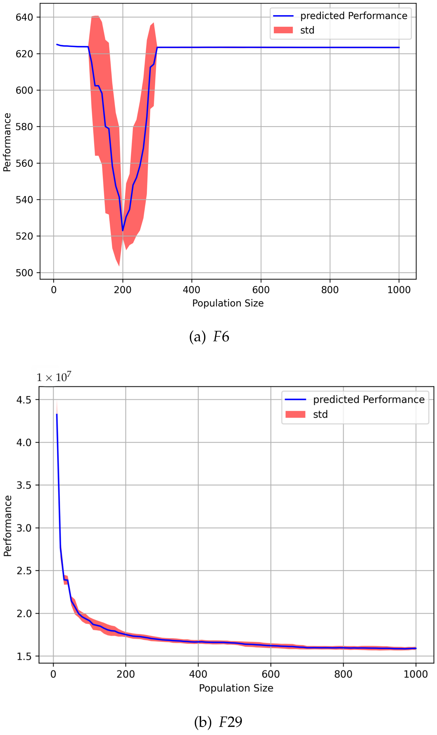
Figure 5 presents the average fitness, with respect to $N_P$, on selected problems. Figure 5 provides additional insights into the relationship between the population size ($N_P$) and the average fitness. Examination of Figure 5a shows that for $F6$, improvement in performance was reported with a population size $N_P$ = 200 individuals, while population sizes of smaller or larger than 200 demonstrated relatively worse performance. In contrast, Figure 5b suggests that an increase in the population size had a positive impact on the performance of $F29$.

Recall that $F6$ is a multimodal problem, while $F29$ is a composition problem. The different shapes of the plots in Figure 5a,b, for different problems further support the findings of Experiment 1, indicating that the optimal population size is problem-dependent. Experimental evidence collected indicates that different behaviors were observed for population sizes across different problem modalities.

To further investigate the mutual interactions and interrelationships between the DE control parameters, pairwise marginals were obtained using the fANOVA technique. Considering all possible pairs of control parameters, the pairwise marginals provide insight into how the variations in one control parameter affect the impact of another control parameter on the algorithm’s performance.

The pairwise marginal results are presented in

Table 2. Pairwise marginals depicting the compound effect of DE control parameters; the highest results are marked in boldface.

Functions	${\mathit{N}}_{\mathit{P}}$-$\mathit{CR}$	F-$\mathit{CR}$	${\mathit{N}}_{\mathit{P}}$-F
$F1$	0.105	0.124	0.030
$F2$	0.061	0.118	0.019
$F3$	0.067	0.038	0.014
$F4$	0.099	0.124	0.024
$F5$	0.175	0.052	0.023
$F6$	0.035	0.002	0.031
$F7$	0.067	0.130	0.017
$F8$	0.077	0.045	0.009
$F9$	0.070	0.044	0.011
$F10$	0.085	0.024	0.007
$F11$	0.139	0.033	0.014
$F12$	0.264	0.042	0.020
$F13$	0.089	0.111	0.019
$F14$	0.067	0.131	0.020
$F15$	0.125	0.118	0.047
$F16$	0.313	0.055	0.020
$F17$	0.236	0.043	0.023
$F18$	0.096	0.073	0.045
$F19$	0.092	0.079	0.058
$F20$	0.346	0.024	0.045
$F21$	0.174	0.113	0.015
$F22$	0.126	0.028	0.031
$F23$	0.089	0.079	0.026
$F24$	0.042	0.083	0.010
$F25$	0.093	0.102	0.017
$F26$	0.235	0.081	0.042
$F27$	0.126	0.175	0.018
$F28$	0.119	0.128	0.019
$F29$	0.101	0.080	0.031
$F30$	0.265	0.080	0.024
Average	0.133	0.079	0.024
Std.Dev.	0.064	0.035	0.010

.

It is evident that different pairwise marginals were obtained for different problems, which suggests that the interactions between DE control parameters are problem-specific and that parameter tuning approaches need to be problem-tailored. Moreover, the results reveal that, on average, the combined influence of the population size $N_P$ and the crossover rate $CR$ was found to be marginally the most important across the CEC 2014 problems. Specifically, the combined effect of $N_P$ and $CR$ on the DE performance exhibited the highest impact on DE performance for twenty problems, while the combined effect of F and $CR$ had the highest impact on DE performance for ten problems. Notably, the combination of $N_P$ and F was not found to have a high impact for any of the problems.

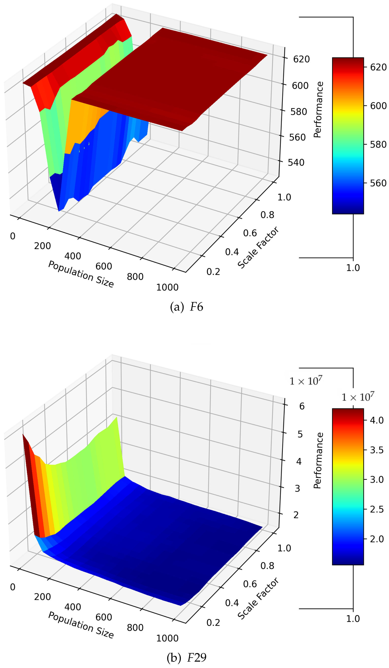
To further investigate the interaction effects of the population size with respect to other control parameters, the pairwise marginal plots between $N_P$ and F, and between $N_P$ and $CR$ are depicted in Figure 6 and Figure 7, respectively.

Figure 6 further supports the fANOVA results, demonstrating that the combined effect of $N_P$ and F was less influential on overall DE performance. Conversely, the plots in Figure 7 indicate that the influence of the population size $N_P$ was significantly higher for smaller values of the $CR$ compared to larger values. Such interaction effects could not be demonstrated by the single marginal plots and should be considered when control parameters are configured.

Two significant findings arise from the aforementioned analysis: Firstly, the evidence collected demonstrates that the behavior of the population size varies across different problem modalities, and there are notable interaction effects between $N_P$, $CR$, and F. As a result, it can be reasonably claimed that tuning of control parameters individually without considering the inter-dependencies with other control parameters may not result in an optimal parameter configuration and hence may not lead to optimized performance. Secondly, the research findings from Experiment 2 further highlight the necessity of incorporating the characteristics of the search space when control parameters are tuned. Different problems may exhibit different complexities, requiring tailored parameter configurations to attain optimal performance.

In summary, based on the analysis conducted in the second experiment on the CEC 2014 problems, the population size as a control parameter has demonstrated critical significance, in alignment with the findings of the past studies on the DE algorithm. The results provide empirical evidence that the population size was the second most influential control parameter with respect to overall fitness. Moreover, the effect of the interaction between $N_P$ and $CR$ was found to be the most influential on DE performance. The observed interaction results revealed that $N_P$ as a control parameter is of critical importance for small values of $CR$ compared to large values.

8. Summary Discussion and Implications

This section summarizes the key findings based on the empirical analysis carried out in the pervious section. The section also provides the implications of these findings for practitioners.

8.1. Summary of Key Findings

One of the key findings of this research challenges the credibility and effectiveness of the existing guidelines for setting the population size in the DE algorithm. The results suggest that setting the population size based on problem dimension or using a fixed value cannot be considered an optimal approach. The findings further indicate that a “one-size-fits-all” strategy for setting population size in the DE algorithm carries the risk of overestimating the initial population and can lead to excessively large populations. Notably, large populations have diminishing effects on the DE algorithm, aside from increasing the computational burden. Moreover, population size emerged as the second most influential parameter affecting DE performance, interacting critically with other DE control parameters, particularly $CR$, which was shown to be of critical importance, especially for small populations. The results highlight the necessity of problem-tailored population size setting. In the following subsection, the implications for practitioners are discussed.

8.2. Implications for Practitioners

Based on the results and discussions presented above, the following recommendations are provided for practitioners to consider:

• Focus on moderate population sizes and avoid excessively large ones: Choose moderate population sizes. The results indicate that excessively large population sizes do not necessarily enhance performance and can even hamper it. Practitioners should be mindful of the potential drawbacks of significant increments in population size, and avoid unnecessary wastage of computational costs. Large population sizes should only be considered for highly complex problems in high-dimensional spaces, where they may be specifically required.
• Population size limit: The results indicate the existence of a population size threshold beyond which performance starts to deteriorate. Practitioners are advised to pay close attention to this threshold by fine-tuning the population size and making careful, incremental adjustments.
• Avoid tuning parameters in isolation and recognize the impact of parameters interactions: Based on the findings from fANOVA, practitioners should recognize the significant interactions between DE control parameters. Tuning control parameters individually can fail to capture the interactions between them, leading to a misinterpretation of performance variations that arise from these interactions. Specifically, the crossover rate plays a pivotal role affecting DE performance, especially when using small population sizes.
• Consider problem-specific population size adaptations: The findings in this study indicate that different problems require different population size settings. Practitioners working with complex, multimodal, or composition problems should experiment using population sizes beyond typical recommendations to achieve optimized performance. This is specifically advisable for extremely complex problems in high-dimensional spaces.
• Avoid relying on rule-of-thumb guidelines for setting the population size: The results challenge the commonly used guidelines for setting the population size in the DE algorithm. Practitioners should avoid relying solely on these rules and instead determine the most suitable parameters for their specific problem by conducting on-the-run analysis during the optimization process. It is essential to consider the unique characteristics of the problem at hand.
• Consider the priority of the control parameters: The results indicate that, for certain problems, the population size holds the highest importance and thus critically affects the DE performance compared to other parameters, such as with the Weierstrass function (F6). Practitioners dealing with similarly complex landscapes should prioritize fine-tuning the population size compared to other DE parameters.
• Apply proper statistical testing for robust population size evaluations: Practitioners are advised to use appropriate statistical validation techniques to ensure the accurate evaluation of an optimal population size. This is particularly crucial when testing and comparing different population sizes, where a two-step statistical analysis is necessary (such as the Friedman–Shaffer test).
• Leverage fANOVA to provide insights into DE control parameters: The fANOVA approach utilized in this study offers a robust method for assessing the importance of control parameters and provides insights into their interrelationships. Practitioners working with DE can adopt similar statistical techniques to gain a deeper understanding of which parameters to prioritize and identify critical relationships between control parameters that require special attention for the specific problem at hand.
• Consider complementary approaches: In related studies, different approaches have been explored to optimize DE control parameters including the population size. For instance, Kok and Rajendran [97] used empirical data and applied linear regression to formulate an equation for determining the optimal population size, and polynomial regression for other DE control parameters in a real-world problem. Additionally, the study by Centeno-Telleria et al. [114] utilized an artificial neural network (ANN) to establish connections between DE performance and control parameter values, extracting the optimal values for control parameters, including the population size. While these studies provide advanced approaches, the current study offers a more comprehensive experimental analysis. Practitioners can gain further insight by combining the findings of this study with advanced approaches to achieve insightful population size tuning for the DE algorithm. Future research could also explore the integration of these advanced approaches to enhance DE performance across diverse problem domains.
• Reassess setting the initial population size for DE strategies with adaptive population: Practitioners are advised to pay special attention when designing and configuring DE strategies with adaptive populations. The experimental results presented in this study suggest that increasing the population size beyond a threshold limit hampers DE performance. Moreover, the interactions between DE control parameters highlight the need for careful tuning, particularly the interaction between $NP$ and $CR$ for small population sizes.

9. Conclusions

The current approaches to set the population size in the differential evolution (DE) algorithm based on problem dimensionality or as a subjective fixed value lack the reliability and precision necessary for optimizing DE performance across diverse problems complexities. This study meticulously examined the efficacy of existing guidelines for setting the population size within the DE algorithm across various problem types and modalities utilizing the CEC 2014 benchmark suite. Moreover, the relative importance and interrelationships between DE control parameters were investigated using the functional analysis of variance (fANOVA) approach.

The analysis revealed that conventional guidelines may often lead to over-estimations of initial populations and hence highlights the need for a reevaluation of how population sizes are determined in the DE algorithms. Furthermore, a link between population size and fitness landscape characteristics was found, revealing that different problems favor various population sizes. Specifically complex composition problems were found to benefit from larger population sizes, a finding not previously emphasized in the DE literature. Additionally, the investigation highlighted the paramount importance of the population size as a critical control parameter in the DE algorithm, ranking its significance second only to the crossover rate $\left(CR\right)$ and preceding the scale factor $\left(F\right)$ in terms of impact. Notably, the crossover rate contributed 43.6% to the total fitness variation, making it the most influential control parameter, followed by the population size at 21.9%. In contrast, the scale factor accounted for only 3% of the fitness variation. These results highlight the critical need to carefully tune DE control parameters for optimal DE performance. This study also explores the interrelationships between DE control parameters and identifies the crossover rate as the most influential factor affecting fitness variance in the DE algorithm. Moreover, the interaction between population size and the crossover rate shows a significant influence on the DE performance, with larger population sizes proving particularly advantageous at lower crossover rates to optimize DE performance.

An important and potential direction for future research involves conducting experiments on real-world problems. Currently, the focus of the study is on the CEC 2014 benchmark problems, which may not fully capture the diversity of real-world problem modalities. Moreover, a promising future work is the integration of machine learning techniques (such as regression trees and random forests) to predict optimal population size preemptively. Another direction for future work could also focus on developing adaptive DE strategies to dynamically adjust the population size based on fitness landscape characteristics of problems and convergence. This involves investigating the relationship between the population diversity and convergence speed across problems of various fitness landscape characteristics, particularly incorporating additional fitness landscape characteristics, such as ruggedness, deception, and searchability. Additionally, a potential avenue for future work is to further investigate the interaction between DE control parameters considering a broader spectrum of problems of various complexities including real-world problems. This investigation is not only needed to gain a better understanding of DE control parameters optimization but also to facilitate the development of more sophisticated, problem-specific guidelines for setting population sizes in the DE algorithms.

References

1. Feurer, M.; Hutter, F. Hyperparameter optimization. In Automated Machine Learning: Methods, Systems, Challenges; Hutter, F., Kotthoff, L., Vanschoren, J., Eds.; Springer: Cham, Switzerland, 2019; pp. 3–33. [Google Scholar]
2. Spears, W.M.; De Jong, K.A.; Bäck, T.; Fogel, D.B.; De Garis, H. An overview of evolutionary computation. In Proceedings of the European Conference on Machine Learning (ECML-93), Vienna, Austria, 5–7 April 1993; pp. 442–459. [Google Scholar]
3. Chena, T.; Tangb, K.; Chenb, G.; Yaob, X. A large population size can be unhelpful in evolutionary algorithms. Theor. Comput. Sci. 2012, 436, 54–70. [Google Scholar] [CrossRef]
4. Gotshall, S.; Rylander, B. Optimal population size and the genetic algorithm. Population 2002, 100, 900–904. [Google Scholar]
5. Mallipeddi, R.; Suganthan, P. Empirical study on the effect of population size on differential evolution algorithm. In Proceedings of the IEEE Congress on Evolutionary Computation, Hong Kong, China, 1–6 June 2008; pp. 3663–3670. [Google Scholar]
6. Mallipeddi, R.; Suganthan, P.N. Differential evolution algorithm with ensemble of parameters and mutation and crossover strategies. In Proceedings of the Swarm, Evolutionary, and Memetic Computing (SEMCCO), Chennai, India, 16–18 December 2010; pp. 71–78. [Google Scholar]
7. Eiben, A.; Smith, J. Introduction to Evolutionary Computing; Springer: Berlin/Heidelberg, Germany, 2003. [Google Scholar]
8. Storn, R. On the usage of differential evolution for function optimization. In Proceedings of the North American Fuzzy Information Processing, Berkeley, CA, USA, 19–22 June 1996; pp. 519–523. [Google Scholar]
9. Storn, R.; Price, K. Differential evolution—A simple and efficient heuristic for global optimization over continuous spaces. J. Glob. Optim. 1997, 11, 341–359. [Google Scholar] [CrossRef]
10. Zaharie, D. Critical values for the control parameters of differential evolution algorithms. In Proceedings of the 8th International Mendel Conference on Soft Computing, Brno, Czech Republic, 5–7 June 2002; pp. 62–67. [Google Scholar]
11. Zielinski, K.; Laur, R. Parameter adaptation for differential evolution with design of experiments. In Proceedings of the IASTED International Conference on Computational Intelligence, San Francisco, CA, USA, 20–22 November 2006; pp. 216–221. [Google Scholar]
12. Neri, F.; Tirronen, V. Recent advances in differential evolution: A survey and experimental analysis. Artif. Intell. Rev. 2010, 33, 61–106. [Google Scholar] [CrossRef]
13. Das, S.; Suganthan, P.N. Differential evolution: A survey of the state-of-the-art. IEEE Trans. Evol. Comput. 2011, 15, 4–31. [Google Scholar] [CrossRef]
14. Lampinen, J.; Zelinka, I. On stagnation of the differential evolution algorithm. In Proceedings of the 6th International Mendel Conference on Soft Computing, Brno, Czech Republic, 7–9 June 2000; pp. 76–83. [Google Scholar]
15. Malan, K.M.; Engelbrecht, A.P. Algorithm comparisons and the significance of population size. In Proceedings of the IEEE Congress on Evolutionary Computation, Hong Kong, China, 1–6 June 2008; pp. 914–920. [Google Scholar]
16. Piotrowski, A.P. Review of differential evolution population size. Swarm Evol. Comput. 2017, 32, 1–24. [Google Scholar] [CrossRef]
17. Chen, S.; Montgomery, J.; Bolufé-Röhler, A. Measuring the curse of dimensionality and its effects on particle swarm optimization and differential evolution. Appl. Intell. 2015, 42, 514–526. [Google Scholar] [CrossRef]
18. Piotrowski, A.P.; Napiorkowski, J.J.; Piotrowska, A.E. Population size in particle swarm optimization. Swarm Evol. Comput. 2020, 58, 100718. [Google Scholar] [CrossRef]
19. Brest, J.; Sepesy Maučec, M. Population Size Reduction for the Differential Evolution Algorithm. Appl. Intell. 2008, 29, 228–247. [Google Scholar] [CrossRef]
20. Brest, J.; Maučec, M.S. Self-adaptive differential evolution algorithm using population size reduction and three strategies. Soft Comput. 2011, 15, 2157–2174. [Google Scholar] [CrossRef]
21. Yang, M.; Cai, Z.; Guan, J.; Gong, W. Differential evolution with improved population reduction. In Proceedings of the 13th Annual Conference Companion on Genetic and Evolutionary Computation, Dublin, Ireland, 12–16 July 2011; pp. 143–144. [Google Scholar]
22. Zamuda, A.; Brest, J.; Mezura-Montes, E. Structured population size reduction differential evolution with multiple mutation strategies on CEC 2013 real parameter optimization. In Proceedings of the IEEE Congress on Evolutionary Computation, Cancun, Mexico, 20–23 June 2013; pp. 1925–1931. [Google Scholar]
23. Yang, M.; Guan, J.; Cai, Z.; Li, C. Differential evolution based on population reduction with minimum distance. In Proceedings of the 2013 Sixth International Conference on Advanced Computational Intelligence (ICACI), Hangzhou, China, 19–21 October 2013; pp. 96–101. [Google Scholar]
24. Poláková, R.; Bujok, P. Adaptation of population size in differential evolution algorithm: An experimental comparison. In Proceedings of the 2018 25th International Conference on Systems, Signals and Image Processing (IWSSIP), Maribor, Slovenia, 20–22 June 2018; pp. 1–5. [Google Scholar]
25. Cheng, L.; Wang, Y.; Wang, C.; Mohamed, A.W.; Xiao, T. Adaptive differential evolution based on successful experience information. IEEE Access 2020, 8, 164611–164636. [Google Scholar] [CrossRef]
26. Fister, I.; Iglesias, A.; Galvez, A.; Fister, D.; Fister, I. Parallel differential evolution with variable population size for global optimization. In Proceedings of the 15th International Conference on Soft Computing Models in Industrial and Environmental Applications (SOCO 2020), Seville, Spain, 5–7 September 2020; pp. 89–99. [Google Scholar]
27. Brest, J.; Maučec, M.S.; Bošković, B. Self-adaptive differential evolution algorithm with population size reduction for single objective bound-constrained optimization: Algorithm j21. In Proceedings of the 2021 IEEE Congress on Evolutionary Computation (CEC), Kraków, Poland, 28 June–1 July 2021; pp. 817–824. [Google Scholar]
28. Teo, J. Differential Evolution with Self-adaptive Populations. In Knowledge-Based Intelligent Information and Engineering Systems. KES 2005; Lecture Notes in Computer Science; Khosla, R., Howlett, R., Jain, L., Eds.; Springer: Berlin/Heidelberg, Germany, 2005; Volume 3681. [Google Scholar]
29. Wang, H.; Rahnamayan, S.; Wu, Z. Adaptive Differential Evolution with Variable Population Size for Solving High-Dimensional Problems. In Proceedings of the 2011 IEEE Congress on Evolutionary Computation (CEC), New Orleans, LA, USA, 5–8 June 2011; pp. 2626–2632. [Google Scholar]
30. Yang, M.; Cai, Z.; Li, C.; Guan, J. An improved adaptive differential evolution algorithm with population adaptation. In Proceedings of the 15th Annual Conference on Genetic and Evolutionary Computation, Amsterdam, The Netherlands, 6–10 July 2013; pp. 145–152. [Google Scholar]
31. Zhu, W.; Tang, Y.; Fang, J.A.; Zhang, W. Adaptive population tuning scheme for differential evolution. Inf. Sci. 2013, 223, 164–191. [Google Scholar] [CrossRef]
32. Choi, T.J.; Ahn, C.W. An Adaptive Differential Evolution Algorithm with Automatic Population Resizing for Global Numerical Optimization. In Bio-Inspired Computing—Theories and Applications; Communications in Computer and Information Science; Pan, L., Păun, G., Pérez-Jiménez, M., Song, T., Eds.; Springer: Berlin/Heidelberg, Germany, 2014; Volume 472. [Google Scholar]
33. Shi, E.C.; Leung, F.H.; Law, B.N. Differential Evolution with adaptive population size. In Proceedings of the 2014 19th International Conference on Digital Signal Processing, Hong Kong, China, 20–23 August 2014; pp. 876–881. [Google Scholar]
34. Aalto, J.; Lampinen, J. A population adaptation mechanism for differential evolution algorithm. In Proceedings of the 2015 IEEE Symposium Series on Computational Intelligence, Cape Town, South Africa, 7–10 December 2015; pp. 1514–1521. [Google Scholar]
35. Brown, C.; Jin, Y.; Leach, M.; Hodgson, M. μJADE: Adaptive differential evolution with a small population. Soft Comput. 2016, 20, 4111–4120. [Google Scholar] [CrossRef]
36. Wong, I.; Liu, W.; Ho, C.M.; Ding, X. Continuous adaptive population reduction (CAPR) for differential evolution optimization. SLAS Technol. 2017, 22, 289–305. [Google Scholar] [CrossRef]
37. Poláková, R.; Tvrdík, J.; Bujok, P. Adaptation of population size according to current population diversity in differential evolution. In Proceedings of the 2017 IEEE Symposium Series on Computational Intelligence (SSCI), Honolulu, HI, USA, 27 November–1 December 2017; IEEE: Piscataway, NJ, USA, 2017; pp. 1–8. [Google Scholar]
38. Poláková, R.; Tvrdík, J.; Bujok, P. Differential evolution with adaptive mechanism of population size according to current population diversity. Swarm Evol. Comput. 2019, 50, 100519. [Google Scholar] [CrossRef]
39. Zhan, Z.H.; Zhang, J. Co-evolutionary Differential Evolution with Dynamic Population Size and Adaptive Migration Strategy. In Proceedings of the 13th Annual Conference Companion on Genetic and Evolutionary Computation, Dublin, Ireland, 12–16 July 2011; pp. 211–212. [Google Scholar]
40. Ali, M.Z.; Awad, N.H.; Suganthan, P.N.; Reynolds, R.G. An adaptive multipopulation differential evolution with dynamic population reduction. IEEE Trans. Cybern. 2016, 47, 2768–2779. [Google Scholar] [CrossRef]
41. Li, K.; Fu, X.; Wang, F.; Jalil, H. A dynamic population reduction differential evolution algorithm combining linear and nonlinear strategy piecewise functions. Concurr. Comput. Pract. Exper. 2022, 34, e6773. [Google Scholar] [CrossRef]
42. Brest, J.; Greiner, S.; Boskovic, B.; Mernik, M.; Zumer, V. Self-adapting control parameters in differential evolution: A comparative study on numerical benchmark problems. IEEE Trans. Evol. Comput. 2006, 10, 646–657. [Google Scholar] [CrossRef]
43. Teng, N.S.; Teo, J.; Hijazi, M.H.A. Self-adaptive population sizing for a tune-free differential evolution. Soft Comput. 2009, 13, 709–724. [Google Scholar] [CrossRef]
44. Sing, T.N.; Teo, J. Evolutionary and Population Dynamics of 3 Parents Differential Evolution (3PDE) Using Self-Adaptive Tuning Methodologies. Nat. Comput. 2011, 10, 507–526. [Google Scholar] [CrossRef]
45. Zamuda, A.; Brest, J. Population Reduction Differential Evolution with Multiple Mutation Strategies in Real World Industry Challenges. In Swarm and Evolutionary Computation. EC SIDE 2012; Lecture Notes in Computer Science; Rutkowski, L., Korytkowski, M., Scherer, R., Tadeusiewicz, R., Zadeh, L., Zurada, J., Eds.; Springer: Berlin/Heidelberg, Germany, 2012; Volume 7269. [Google Scholar]
46. Elsayed, S.M.; Sarker, R.A.; Ray, T. Parameters adaptation in differential evolution. In Proceedings of the IEEE Congress on Evolutionary Computation, Brisbane, QLD, Australia, 10–15 June 2012; pp. 1–8. [Google Scholar]
47. Brest, J.; Bošković, B.; Zamuda, A.; Fister, I.; Maučec, M.S. Self-adaptive Differential Evolution Algorithm with a Small and Varying Population Size. In Proceedings of the 2012 IEEE Congress on Evolutionary Computation, Brisbane, QLD, Australia, 10–15 June 2012; pp. 1–8. [Google Scholar]
48. Zhao, S.; Wang, X.; Chen, L.; Zhu, W. A novel self-adaptive differential evolution algorithm with population size adjustment scheme. Arab. J. Sci. Eng. 2014, 39, 6149–6174. [Google Scholar] [CrossRef]
49. Yang, M.; Guan, J.; Cai, Z.; Li, C. A self-adaptive differential evolutionary algorithm based on population reduction with minimum distance. Int. J. Innov. Comput. Appl. 2014, 6, 13–24. [Google Scholar] [CrossRef]
50. Budiman, H.; Wang, S.L.; Morsidi, F.; Ng, T.F.; Neoh, S.C. Self-adaptive ensemble-based differential evolution with enhanced population sizing. In Proceedings of the 2020 2nd International Conference on Cybernetics and Intelligent System (ICORIS), Manado, Indonesia, 27–28 October 2020; IEEE: Piscataway, NJ, USA, 2020; pp. 1–6. [Google Scholar]
51. Brest, J.; Zamuda, A.; Boskovic, B.; Maucec, M.S.; Zumer, V. High-Dimensional Real-Parameter Optimization Using Self-Adaptive Differential Evolution Algorithm with Population Size Reduction. In Proceedings of the 2008 IEEE Congress on Evolutionary Computation (IEEE World Congress on Computational Intelligence), Hong Kong, China, 1–6 June 2008; pp. 2032–2039. [Google Scholar]
52. Brest, J.; Maučec, M.S.; Bošković, B. Single objective real-parameter optimization: Algorithm jSO. In Proceedings of the 2017 IEEE Congress on Evolutionary Computation (CEC), Donostia/San Sebastian, Spain, 5–8 June 2017; IEEE: Piscataway, NJ, USA, 2017; pp. 1311–1318. [Google Scholar]
53. Mohamed, A.K.; Mohamed, A.W.; Elfeky, E.Z.; Saleh, M. Enhancing AGDE algorithm using population size reduction for global numerical optimization. In Proceedings of the International Conference on Advanced Machine Learning Technologies and Applications (AMLTA), Cairo, Egypt, 22–24 February 2018; pp. 62–72. [Google Scholar]
54. Di Carlo, M.; Vasile, M.; Minisci, E. Adaptive multi-population inflationary differential evolution. Soft Comput. 2020, 24, 3861–3891. [Google Scholar] [CrossRef]
55. Meng, Z.; Chen, Y.; Li, X.; Lin, F. PADE-NPC: Parameter adaptive differential evolution with novel parameter control for single-objective optimization. IEEE Access 2020, 8, 139460–139478. [Google Scholar] [CrossRef]
56. Brest, J.; Maučec, M.S.; Bošković, B. Differential evolution algorithm for single objective bound-constrained optimization: Algorithm j2020. In Proceedings of the 2020 IEEE Congress on Evolutionary Computation (CEC), Glasgow, UK, 19–24 July 2020; pp. 1–8. [Google Scholar]
57. Zhang, Y.; Dai, G.; Peng, L.; Wang, M. Enhancing differential evolution algorithm through a population size adaptation strategy. Nat. Comput. 2021, 22, 379–392. [Google Scholar] [CrossRef]
58. Zheng, L.; Luo, S. Adaptive Differential Evolution Algorithm Based on Fitness Landscape Characteristic. Mathematics 2022, 10, 1511. [Google Scholar] [CrossRef]
59. Zhang, X.; Liu, Q.; Qu, Y. An adaptive differential evolution algorithm with population size reduction strategy for unconstrained optimization problem. Appl. Soft Comput. 2023, 138, 110209. [Google Scholar] [CrossRef]
60. Tian, M.; Gao, Y.; He, X.; Zhang, Q.; Meng, Y. Differential Evolution with Group-Based Competitive Control Parameter Setting for Numerical Optimization. Mathematics 2023, 11, 3355. [Google Scholar] [CrossRef]
61. Li, C.; Sun, G.; Deng, L.; Qiao, L.; Yang, G. A population state evaluation-based improvement framework for differential evolution. Inf. Sci. 2023, 629, 15–38. [Google Scholar] [CrossRef]
62. Liu, J.; Lampinen, J. Population size adaptation for differential evolution algorithm using fuzzy logic. In Proceedings of the Intelligent Systems Design and Applications Conference, Budapest, Hungary, 6–8 April 2003; pp. 425–436. [Google Scholar]
63. Meng, Z.; Pan, J.S.; Zheng, W.m.; Li, X. An improved linear population size reduction based parameters with adaptive learning mechanism differential evolution (iLPALMDE) for real-parameter single objective black box optimization. In Proceedings of the Advances in Smart Vehicular Technology, Transportation, Communication and Applications: Proceedings of the Second International Conference on Smart Vehicular Technology, Transportation, Communication and Applications, Mount Emei, China, 25–28 October 2019; pp. 477–484. [Google Scholar]
64. Zeng, Z.; Zhang, M.; Zhang, H.; Hong, Z. Improved differential evolution algorithm based on the sawtooth-linear population size adaptive method. Inf. Sci. 2022, 608, 1045–1071. [Google Scholar] [CrossRef]
65. Yi, W.; Chen, Y.; Pei, Z.; Lu, J. Adaptive differential evolution with ensembling operators for continuous optimization problems. Swarm Evol. Comput. 2022, 69, 100994. [Google Scholar] [CrossRef]
66. Li, Y.; Wang, S.; Yang, B.; Chen, H.; Wu, Z.; Yang, H. Population reduction with individual similarity for differential evolution. Artif. Intell. Rev. 2023, 56, 3887–3949. [Google Scholar] [CrossRef]
67. Song, Y.; Cai, X.; Zhou, X.; Zhang, B.; Chen, H.; Li, Y.; Deng, W.; Deng, W. Dynamic hybrid mechanism-based differential evolution algorithm and its application. Expert Syst. Appl. 2023, 213, 118834. [Google Scholar] [CrossRef]
68. Li, Y.; Han, T.; Tang, S.; Huang, C.; Zhou, H.; Wang, Y. An improved differential evolution by hybridizing with estimation-of-distribution algorithm. Inf. Sci. 2023, 619, 439–456. [Google Scholar] [CrossRef]
69. Gu, Q.; Li, S.; Liao, Z. Solving nonlinear equation systems based on evolutionary multitasking with neighborhood-based speciation differential evolution. Expert Syst. Appl. 2024, 238, 122025. [Google Scholar] [CrossRef]
70. Yang, Q.; Qiao, Z.Y.; Xu, P.; Lin, X.; Gao, X.D.; Wang, Z.J.; Lu, Z.Y.; Jeon, S.W.; Zhang, J. Triple competitive differential evolution for global numerical optimization. Swarm Evol. Comput. 2024, 84, 101450. [Google Scholar] [CrossRef]
71. Salgotra, R.; Gandomi, A.H. A novel multi-hybrid differential evolution algorithm for optimization of frame structures. Sci. Rep. 2024, 14, 4877. [Google Scholar] [CrossRef] [PubMed]
72. Al-Dabbagh, R.D.; Neri, F.; Idris, N.; Baba, M.S. Algorithmic design issues in adaptive differential evolution schemes: Review and taxonomy. Swarm Evol. Comput. 2018, 43, 284–311. [Google Scholar] [CrossRef]
73. Price, K. An introduction to differential evolution. In New Ideas in Optimization; Corne, D., Dorigo, M., Glover, F., Eds.; McGraw-Hill: London, UK, 1999; pp. 79–108. [Google Scholar]
74. Gämperle, R.; Müller, S.D.; Koumoutsakos, P. A parameter study for differential evolution. In Proceedings of the Conference in Neural Networks and Applications, Fuzzy Sets and Fuzzy Systems and Evolutionary Computation, Interlaken, Switzerland, 11–15 February 2002; pp. 293–298. [Google Scholar]
75. Liu, J.; Lampinen, J. A fuzzy adaptive differential evolution algorithm. Soft Comput. 2005, 9, 448–462. [Google Scholar] [CrossRef]
76. Ali, M.; Fatti, L. A differential free point generation scheme in the differential evolution algorithm. J. Glob. Optim. 2006, 35, 551–572. [Google Scholar] [CrossRef]
77. Ali, M. Differential evolution with preferential crossover. Eur. J. Oper. Res. 2007, 181, 1137–1147. [Google Scholar] [CrossRef]
78. Piotrowski, A.P.; Napiórkowski, J.J. The grouping differential evolution algorithm for multi-dimensional optimization problems. Control Cybern. 2010, 39, 527–550. [Google Scholar]
79. Mohamed, A.W.; Sabry, H.Z. Constrained optimization based on modified differential evolution algorithm. Inf. Sci. 2012, 194, 171–208. [Google Scholar] [CrossRef]
80. Kotyrba, M.; Volna, E.; Bujok, P. Unconventional modelling of complex system via cellular automata and differential evolution. Swarm Evol. Comput. 2015, 25, 52–62. [Google Scholar] [CrossRef]
81. Sarkar, S.; Das, S.; Chaudhuri, S.S. Hyper-spectral image segmentation using Rényi entropy based multi-level thresholding aided with differential evolution. Expert Syst. Appl. 2016, 50, 120–129. [Google Scholar] [CrossRef]
82. Goudos, S.K.; Baltzis, K.B.; Antoniadis, K.; Zaharis, Z.D.; Hilas, C.S. A comparative study of common and self-adaptive differential evolution strategies on numerical benchmark problems. Procedia Comput. Sci. 2011, 3, 83–88. [Google Scholar] [CrossRef]
83. Neri, F.; Tirronen, V. On memetic differential evolution frameworks: A study of advantages and limitations in hybridization. In Proceedings of the IEEE Congress on Computational Intelligence, Hong Kong, China, 1–6 June 2008; pp. 2135–2142. [Google Scholar]
84. Dragoi, E.N.; Curteanu, S.; Leon, F.; Galaction, A.I.; Cascaval, D. Modeling of oxygen mass transfer in the presence of oxygen-vectors using neural networks developed by differential evolution algorithm. Eng. Appl. Artif. Intell. 2011, 24, 1214–1226. [Google Scholar] [CrossRef]
85. Bellman, R.E. Dynamic Programming; Princeton University Press: Princeton, NJ, USA, 1957. [Google Scholar]
86. Das, R.; Prasad, D.K. Prediction of porosity and thermal diffusivity in a porous fin using differential evolution algorithm. Swarm Evol. Comput. 2015, 23, 27–39. [Google Scholar] [CrossRef]
87. Apolloni, J.; García-Nieto, J.; Alba, E.; Leguizamón, G. Empirical evaluation of distributed differential evolution on standard benchmarks. Appl. Math. Comput. 2014, 236, 351–366. [Google Scholar] [CrossRef]
88. Tasgetiren, M.F.; Pan, Q.K.; Suganthan, P.N.; Buyukdagli, O. A variable iterated greedy algorithm with differential evolution for the no-idle permutation flowshop scheduling problem. Comput. Oper. Res. 2013, 40, 1729–1743. [Google Scholar] [CrossRef]
89. Wang, Y.; Li, H.X.; Huang, T.; Li, L. Differential evolution based on covariance matrix learning and bimodal distribution parameter setting. Appl. Soft Comput. 2014, 18, 232–247. [Google Scholar] [CrossRef]
90. Song, Y.; Zhao, G.; Zhang, B.; Chen, H.; Deng, W.; Deng, W. An enhanced distributed differential evolution algorithm for portfolio optimization problems. Eng. Appl. Artif. Intell. 2023, 121, 106004. [Google Scholar] [CrossRef]
91. Li, Y.L.; Zhan, Z.H.; Gong, Y.J.; Chen, W.N.; Zhang, J.; Li, Y. Differential evolution with an evolution path: A DEEP evolutionary algorithm. IEEE Trans. Cybern. 2014, 45, 1798–1810. [Google Scholar] [CrossRef]
92. Weber, M.; Neri, F.; Tirronen, V. A study on scale factor in distributed differential evolution. Inf. Sci. 2011, 181, 2488–2511. [Google Scholar] [CrossRef]
93. Wu, G.; Mallipeddi, R.; Suganthan, P.N.; Wang, R.; Chen, H. Differential evolution with multi-population based ensemble of mutation strategies. Inf. Sci. 2016, 329, 329–345. [Google Scholar] [CrossRef]
94. Bergstra, J.; Bengio, Y. Random search for hyper-parameter optimization. J. Mach. Learn. Res. 2012, 13, 281–305. [Google Scholar]
95. Hutter, F.; Hoos, H.; Leyton-Brown, K. Identifying key algorithm parameters and instance features using forward selection. In Proceedings of the International Conference on Learning and Intelligent Optimization, Catania, Italy, 7–11 January 2013; pp. 364–381. [Google Scholar]
96. Harrison, K.R.; Ombuki-Berman, B.M.; Engelbrecht, A.P. An analysis of control parameter importance in the particle swarm optimization algorithm. In Advances in Swarm Intelligence; Lecture Notes in Computer Science; Tan, Y., Shi, Y., Niu, B., Eds.; Springer: Cham, Switzerland, 2019; pp. 93–105. [Google Scholar]
97. Kok, K.Y.; Rajendran, P. Differential-evolution control parameter optimization for unmanned aerial vehicle path planning. PLoS ONE 2016, 11, e0150558. [Google Scholar] [CrossRef]
98. Alić, A.; Berkovič, K.; Bošković, B.; Brest, J. Population size in differential evolution. In Proceedings of the Swarm, Evolutionary, and Memetic Computing and Fuzzy and Neural Computing: 7th International Conference, SEMCCO 2019, and 5th International Conference (FANCCO 2019), Maribor, Slovenia, 10–12 July 2019; Revised Selected Papers. pp. 21–30. [Google Scholar]
99. Ahmad, M.F.; Isa, N.A.M.; Lim, W.H.; Ang, K.M. Differential evolution: A recent review based on state-of-the-art works. Alex. Eng. J. 2022, 61, 3831–3872. [Google Scholar] [CrossRef]
100. Hutter, F.; Hoos, H.; Leyton-Brown, K. An efficient approach for assessing hyperparameter importance. In Proceedings of the International Conference on Machine Learning, ICML 2014, Beijing, China, 21– 26 June 2014; pp. 754–762. [Google Scholar]
101. Greff, K.; Srivastava, R.K.; Koutník, J.; Steunebrink, B.R.; Schmidhuber, J. LSTM: A search space odyssey. IEEE Trans. Neural Netw. Learn. Syst. 2016, 28, 2222–2232. [Google Scholar] [CrossRef] [PubMed]
102. Kelz, R.; Dorfer, M.; Korzeniowski, F.; Böck, S.; Arzt, A.; Widmer, G. On the potential of simple framewise approaches to piano transcription. In Proceedings of the International Society for Music Information Retrieval Conference (ISMIR 2016), New York, NY, USA, 7–11 August 2016; pp. 475–481. [Google Scholar]
103. Lago, J.; De Ridder, F.; Vrancx, P.; De Schutter, B. Forecasting day-ahead electricity prices in Europe: The importance of considering market integration. Appl. Energy 2018, 211, 890–903. [Google Scholar] [CrossRef]
104. Ko, B.; Gu, G.; Kim, H.G. Learning with memory-based virtual classes for deep metric learning. In Proceedings of the IEEE/CVF International Conference on Computer Vision, Montreal, QC, Canada, 10–17 October 2021; pp. 11792–11801. [Google Scholar]
105. Hammerla, N.Y.; Halloran, S.; Plötz, T. Deep, convolutional, and recurrent models for human activity recognition using wearables. In Proceedings of the Twenty-Fifth International Joint Conference on Artificial Intelligence, New York, NY, USA, 9–15 July 2016; pp. 1533–1540. [Google Scholar]
106. Van Rijn, J.N.; Hutter, F. Hyperparameter importance across datasets. In Proceedings of the 24th ACM SIGKDD International Conference on Knowledge Discovery & Data Mining, London, UK, 19–23 August 2018; pp. 2367–2376. [Google Scholar]
107. Carolus, T.G.; Engelbrecht, A.P. Multi-guide particle swarm optimisation control parameter importance in high dimensional spaces. In Proceedings of the International Conference on Swarm Intelligence, Shenzhen, China, 17–21 July 2021; pp. 185–198. [Google Scholar]
108. Liang, J.; Qu, B.; Suganthan, P.; Hernández-Díaz, A. Problem Definitions and Evaluation Criteria for the CEC 2013 Special Session on Real-Parameter Optimization; Technical Report 201212; Computational Intelligence Laboratory, Zhengzhou University, China and Nanyang Technological University: Singapore, 2013. [Google Scholar]
109. Liang, J.; Qu, B.; Suganthan, P. Problem Definitions and Evaluation Criteria for the CEC 2014 Special Session and Competition on Single Objective Real-Parameter Numerical optimization; Technical Report 201311; Computational Intelligence Laboratory, Zhengzhou University, China and Nanyang Technological University: Singapore, 2013. [Google Scholar]
110. Liang, J.; Qu, B.; Suganthan, P.; Chen, Q. Problem Definitions and Evaluation Criteria for the CEC 2015 Competition on Learning-Based Real-Parameter Single Objective Optimization; Technical Report 201411A; Computational Intelligence Laboratory, Zhengzhou University, China and Nanyang Technological University: Singapore, 2014. [Google Scholar]
111. Wu, G.; Mallipeddi, R.; Suganthan, P. Problem Definitions and Evaluation Criteria for the CEC 2017 Competition and Special Session on Constrained Single Objective Real-Parameter Optimization; Technical Report; National University of Defense Technology: Changsha, China; Kyungpook National University: Daegu, Republic of Korea; Nanyang Technological University: Singapore, 2016. [Google Scholar]
112. Lang, R.D.; Engelbrecht, A.P. An exploratory landscape analysis-based benchmark suite. Algorithms 2021, 14, 78. [Google Scholar] [CrossRef]
113. Derrac, J.; García, S.; Molina, D.; Herrera, F. A practical tutorial on the use of nonparametric statistical tests as a methodology for comparing evolutionary and swarm intelligence algorithms. Swarm Evol. Comput. 2011, 1, 3–18. [Google Scholar] [CrossRef]
114. Centeno-Telleria, M.; Zulueta, E.; Fernandez-Gamiz, U.; Teso-Fz-Betoño, D.; Teso-Fz-Betoño, A. Differential evolution optimal parameters tuning with artificial neural network. Mathematics 2021, 9, 427. [Google Scholar] [CrossRef]
Figure 1. A Venn diagram illustrating the different approaches to setting the population size in the DE algorithm: problem dimension-related factor, fixed initial population size, and adaptive/self-adaptive population sizes. Adaptive/self-adaptive approaches may increase, decrease, or dynamically adjust the population size during the optimization process.
Applsci 14 09976 g001
Figure 2. Relationship between mean average ranks and the population size for the DE algorithm on CEC 2014 problems for (a) D = 10, (b) D = 30, (c) D = 50, and (d) D = 100, where D is the problem dimension.
Applsci 14 09976 g002aApplsci 14 09976 g002b
Figure 3. Relationship between overall average ranks and population size for 10-, 30-, 50-, and 100-dimensional unimodal, multimodal, hybrid, and composition problems from CEC 2014.
Applsci 14 09976 g003aApplsci 14 09976 g003b
Figure 4. Results of the statistical analysis represented by score for all population sizes with 10-dimensional, 30-dimensional, 50-dimensional, and 100-dimensional problems. (a) D = 10, (b) D = 30, (c) D = 50, and (d) D = 100, where D is the problem dimension.
Applsci 14 09976 g004aApplsci 14 09976 g004b
Figure 5. Average fitness, with respect to N P , on (a) F 6 and (b) F 29 problems. The solid line through the middle indicates the average fitness, and the red area shows the standard deviation.
Applsci 14 09976 g005
Figure 6. Plots for pairwise marginal importance of N P and F for problems (a) F 6 and (b) F 29 .
Applsci 14 09976 g006
Figure 7. Plots for pairwise marginal importance of N P and C R for problems (a) F 6 and (b) F 29 .
Applsci 14 09976 g007