Study of the Impact of Acquisition Parameters on Fault Feature Identification Based on Magnetotelluric Modeling

Abstract

The electromagnetic method is widely used in mineral exploration, geothermal resource exploration, and deep earth structure detection. To improve the resolution and positioning accuracy of magnetotelluric surveys for targets beneath cover, it is essential to utilize forward modeling. This approach allows for a better understanding of the capabilities and limitations of MT in resolving features of different scales. In this paper, we employ forward modeling using the finite element method to simulate a series of continuous fault zones ranging from 100 m to 400 m in width, with varying lengths and dips. These fault zones represent conductive fluid pathways that could be associated with different scales and depths. The forward modeling provides the necessary data and method testing to assess the effectiveness of MT surveys in identifying and resolving such features. Our findings demonstrate that a station spacing of 400 m is optimal for resolving fault zones of various widths. For narrower faults (approximately 100 m), extending the survey line to 12 km or more significantly improves the deep structural inversion of the bounding faults, while an 8 km survey line suffices for wider faults (400 m). However, the vertical extent of these features is less well constrained, with deeper faults appearing broader and inversion depths being notably shallower than actual depths. These results highlight the need for careful interpretation of inversion anomalies, especially when supplementary data from other geophysical methods are lacking. Misinterpretation can lead to inaccurate resource assessments and exploration potential.

1. Introduction

The magnetotelluric (MT) method is an important geophysical technique that utilizes natural alternating electromagnetic fields to investigate the electrical structure of subsurface media. In recent years, the effectiveness of the MT method has been well-demonstrated in resource exploration and geological disaster detection, especially in mineral imaging and geothermal exploration [1,2,3,4,5,6]. With the growing complexity of study areas and the diversification of application environments, the MT method faces increasingly complex challenges, necessitating improved data acquisition and more appropriate inversion methods to achieve high-quality images [7,8,9,10,11]. For instance, in geothermal resource exploration, particularly in northern China [12,13], the distribution of thermal storage is mainly controlled by regional faults. Fault zones are crucial for the transportation and distribution of hot water, as they fracture and saturate the deep Ordovician greywacke, creating channels for the upward conduction of Earth’s deep thermal energy. Therefore, resolving fault zones is the most critical aspect of thermal exploration in this region. To identify faults beneath a cover, broadband MT surveys and long-period MT surveys can be conducted using high-resolution data to enhance the resolution of deep narrow anomalies [14,15,16]. However, MT inversion is inherently multi-resolution, and the inversion model often differs significantly from actual geological structures due to the limited resolution of the MT method and the influence of complex subsurface structures [17,18]. Additionally, sparse low-frequency data points are insufficient to resolve deep fault structures [19,20]. Moreover, different survey designs lead to varying interpretation results, affecting anomaly interpretation and geological assessment. To better understand the relationship between inverted anomalies and tectonics, and to improve the resolution and accuracy of target localization beneath cover, it is essential to design an optimal survey system and assess how line length, station spacing, observation bands, and model grid resolution influence the imaging of target tectonics.

This target-oriented survey design can be achieved through forward modeling, allowing for the pre-determination of the subsurface structure and the evaluation of its resolution in MT inversion. Numerical simulation methods for MT forward modeling mainly include the Finite Element Method (FEM) [21,22], the Spectral Method [23], and the Finite Difference Method (FDM) [20,24]. The Finite Element Method is mostly used due to its high computational accuracy, adaptability to complex structures, and unconditional stability. Previous studies have shown that forward modeling plays a crucial role in optimizing survey design and improving the accuracy of data interpretation [25,26,27,28,29]. Dmitriev, V.I. (2010) [30] considered the influence of the coastal effect on bottom magnetotelluric soundings in the shelf zone, using mathematical modeling of the magnetotelluric field into a two-dimensional medium to choose the most effective methods for calculating the fields near the coastal line. Based on magnetotelluric modeling, Zhang, M.L. (2023) [31] applied the compressive sensing theory to MT acquisition and developed an efficient acquisition approach that uses an optimized station layout with sparse irregular patterns. This new acquisition approach can lead to significant savings in both the acquisition cost and operational time while maximizing the information obtained from a given number of stations. Batista, J.D. (2019) [32] applied genetic algorithms and a local methodology integrating the Gauss-Newton and Conjugate Gradient (GNCG) techniques to test one-dimensional inverse modeling of synthetic magnetotelluric data, leading to the development of a hybrid genetic algorithm for MT inversion of one- and two-dimensional synthetic data. In this study, we constructed a geological model consisting of a set of fault zones with varying widths and dips, representing different scales of conductive fluid pathways associated with mineral or geothermal systems. We designed various survey systems for the geological model using two different model grid schemes. For each scenario, we performed finite element forward modeling to generate synthetic data and conducted MT inversion studies to assess the effectiveness of various survey parameters and model mesh designs in interpreting different fault zones in MT detection. Unlike previous studies that focused on uniform or idealized fault models, this work addresses the challenges posed by heterogeneous geological settings, demonstrating that survey length and data acquisition strategies must be tailored to the specific lithological properties of the region. This approach offers a new perspective on optimizing MT surveys for complex subsurface conditions, which is crucial for improving the precision of fault identification in diverse geological environments.

2. MT Forward Modeling and Parameter Setting

2.1. Fault Model Setup

The two-dimensional geological model consists of three faults, labeled F1, F2, and F3, arranged from west to east (Figure 1). These faults originate from the basement and extend to the shallow layers, forming three distinct low-resistance anomaly zones. F1 has an almost vertical dip, while F2 and F3 dip at angles ranging from 65° to 75°, with all three fault zones having the same width. The geological model was digitized onto a grid with two resolutions: 100 m (Scenario 1) and 200 m (Scenario 2), to analyze the inversion and resolution of fault structures in MT at different resolutions. In Scenario 1, the faults are 100 to 200 m wide, while in Scenario 2, they range from 200 to 400 m wide, with resistivity set to 10 ohm-m in both scenarios. The depth and resistivity of the background layers are consistent across both scenarios, as is the contact ratio between the faults and the background layer. The resistivity of the background layer ranges from 100 to 5000 ohm-m, with the highest resistivity at the basement level.

2.2. Finite Element Modeling

The propagation of electromagnetic waves in subsurface media follows Maxwell’s equations, which form the basis for deriving magnetotelluric forward modeling equations. In a two-dimensional medium, the electromagnetic field can be divided into two independent wave types: one includes the components $E_x$, $H_y$, and $H_z$, known as transverse electric (TE) polarization mode, while the other includes $H_x$, $E_y$, and $E_z$, referred to as transverse magnetic (TM) polarization mode. When solving the numerical solution of the magnetotelluric field in a two-dimensional medium, Maxwell’s equations can be transformed into the following second-order partial differential equations that satisfy $E_x$ and $H_x$ (Equations (1) and (2)) [17,33,34]:

$${\displaystyle \frac{\partial }{\partial y}}\left({\displaystyle \frac{1}{i\omega \mu }}{\displaystyle \frac{\partial E_x}{\partial y}}\right)+({\displaystyle \frac{1}{i\omega \mu }}{\displaystyle \frac{\partial E_x}{\partial z}})+\left(\sigma -i\omega \epsilon \right)E_x=0$$

(1)

$${\displaystyle \frac{\partial }{\partial y}}\left({\displaystyle \frac{1}{\sigma -i\omega \epsilon }}{\displaystyle \frac{\partial H_x}{\partial y}}\right)+({\displaystyle \frac{1}{\sigma -i\omega \epsilon }}{\displaystyle \frac{\partial H_x}{\partial z}})+i\omega \mu H_x=0$$

(2)

Here, $E_x$ represents the horizontal component of the electric field in the x-direction, $H_x$ is the horizontal component of the magnetic field in the x-direction, $\sigma$ is the medium’s electrical conductivity, $\epsilon$ is the dielectric constant, $\mu$ is the magnetic permeability, and $\omega =2\pi f$ is the angular frequency.

Appropriate boundary conditions must be applied to solve Equations (1) and (2). For example, in TM mode, the top boundary AB is typically set at the surface, where the field value $u=H_x$ is set to 1 unit:

$${\left.u\right|}_{AB}=1$$

(3)

Below the bottom boundary CD, homogeneous rock is assumed at a sufficient depth, where the anomalous field generated by local inhomogeneous rock is negligible on CD. This assumption holds when the lower boundary is deep enough and the medium below is homogeneous, allowing the influence of local inhomogeneities to be ignored. At this depth, the propagation equation for electromagnetic waves below the lower boundary is:

$${\left.u\right|}_{CD}=u_0{e}^{-ky}$$

(4)

Here, $u_0$ is a constant, $k=\sqrt{-i\omega \mu \sigma }$ is the propagation coefficient, and $\sigma$ is the rock’s electrical conductivity. Taking the derivative of Equation (4), we get ${\displaystyle \frac{\partial u}{\partial z}}=-ku$. At the lower boundary ${\displaystyle \frac{\partial }{\partial z}}=-{\displaystyle \frac{\partial }{\partial n}}$, the boundary condition at CD is given as:

$${\displaystyle \frac{\partial u}{\partial n}}+ku=0$$

(5)

When the left and right boundaries are sufficiently distant from the inhomogeneity, the anomalous field becomes zero, leading to symmetry in the electromagnetic field:

$${\displaystyle \frac{\partial u}{\partial n}}=0$$

(6)

Based on the above analysis, solving the magnetotelluric field reduces to solving the system of equations formed by partial differential Equation (1) to Equation (2), and the boundary conditions Equations (3)–(6).

$$\begin{array}{l}\nabla \cdot \left(\tau \nabla u\right)+\lambda u=0\hspace{1em}\hspace{1em}\hspace{1em}\in \mathsf{\Omega }\\ u=1\hspace{1em}\hspace{1em}\hspace{1em}\hspace{1em}\hspace{1em} \in \mathrm{A}\mathrm{B}\\ {\displaystyle \frac{\partial u}{\partial n}}=0\hspace{1em}\hspace{1em}\hspace{1em}\hspace{1em} \in \mathrm{A}\mathrm{D},\mathrm{B}\mathrm{C}\\ {\displaystyle \frac{\partial u}{\partial n}}+ku=0\hspace{1em}\hspace{1em}\hspace{1em}\in \mathrm{C}\mathrm{D}\end{array}$$

(7)

For the TE polarization mode: $u=E_x$, $\tau =i\omega \mu$, and $\lambda ={\displaystyle \frac{1}{\sigma -i\omega \epsilon }}$

For the TM polarization mode: $u=H_x$, $\tau ={\displaystyle \frac{1}{\sigma -i\omega \epsilon }}$, and $\lambda =i\omega \mu$.

The finite element method (FEM) is employed to numerically solve this system of equations. To calculate the numerical solution of equation system (7) using the finite element method, we consider its equivalent variational problem:

$$\begin{array}{l}F\left(u\right)={\displaystyle \int \left[\frac{1}{2}\tau {\left(\nabla u\right)}^2-\frac{1}{2}{u}^2\right]}d\mathsf{\Omega }\\ {\left.u\right|}_{AB}=1\\ \delta F\left(u\right)=0\end{array}$$

(8)

The Finite Element Method (FEM) involves dividing the model region $\mathsf{\Omega }$ into a grid of rectangular elements, with bilinear interpolation applied to approximate the field variables using shape functions. This interpolation method strikes a good balance between computational efficiency and accuracy, which is crucial for capturing the smoothness and continuity of the electromagnetic fields. The principles and algorithms of FEM are extensively covered in the literature [17,33,34], and will not be elaborated here. The system of equations is then assembled, incorporating boundary conditions, and solved for field values $u$ at each node. After obtaining these values, the vertical partial derivative ${\displaystyle \frac{\partial u}{\partial z}}$ is computed, which in the TM mode corresponds to ${\displaystyle \frac{\partial H_x}{\partial z}}$. This result is used to calculate the apparent resistivity and impedance phase:

$$\begin{array}{l}{Z}_{yx}=-{\displaystyle \frac{1}{\sigma }}{\displaystyle \frac{\partial H_x}{\partial z}}/H_x\\ {\rho }_{yx}={\displaystyle \frac{1}{\omega \mu }}{\left|Z_{yx}\right|}^2\\ {\varphi }_{yx}=\arctan {\displaystyle \frac{\mathrm{Im}\left[Z_{yx}\right]}{\mathrm{Re}\left[Z_{yx}\right]}}\end{array}$$

(9)

Here, $Z_{yx}$ represents the impedance, ${\rho }_{yx}$ represents the apparent resistivity, and ${\varphi }_{yx}$ represents the impedance phase in the TM polarization mode. In the case of TM polarization, ${\displaystyle \frac{\partial u}{\partial z}}$ corresponds to ${\displaystyle \frac{\partial E_x}{\partial z}}$. Substituting this into Equation (10) yields the apparent resistivity and impedance phase.

$$\begin{array}{l}{Z}_{xy}=E_x/\left({\displaystyle \frac{1}{i\omega \mu }}{\displaystyle \frac{\partial E_x}{\partial z}}\right)\\ {\rho }_{xy}={\displaystyle \frac{1}{\omega \mu }}{\left|Z_{xy}\right|}^2\\ {\varphi }_{xy}=\arctan {\displaystyle \frac{\mathrm{Im}\left[Z_{xy}\right]}{\mathrm{Re}\left[Z_{xy}\right]}}\end{array}$$

(10)

Here, $Z_{xy}$ represents the impedance, ${\rho }_{xy}$ represents the apparent resistivity, and ${\varphi }_{xy}$ represents the impedance phase in the TE polarization mode.

2.3. Forward Modeling Parameters Setting

To assess the ability of various survey parameters to resolve fault zones at different resolutions in MT detection, we devised the following surveys for two model grid scenarios:

(1) The survey length is 14 km, with a frequency band ranging from 0.001 to 1000 Hz, and station spacings of 200 m, 400 m, 600 m, and 800 m, respectively.

(2) The station spacing is 400 m, with a frequency band ranging from 0.001 to 1000 Hz, and survey lengths of 8 km, 10 km, 12 km, and 14 km, respectively.

(3) With a station spacing of 400 m and a survey length of 14 km, the frequency band is divided into two ranges: 0.001 to 1000 Hz for long-period measurements with broadband data, and 0.01 to 100 Hz for relatively narrow-band measurements.

For all survey designs in the two scenarios, forward modeling and inversion parameters remained consistent, except for those comparing survey systems (refer to

Table 1. Mesh parameters for forward modeling.

Station Spacing (m)	Survey Length (km)	Frequency Band (Hz)	No of Air Layers	No of Vertical Cell	Horizontal Cell Size (Scenario 1) (m)	Horizontal Cell Size (Scenario 2) (m)
200	14	0.001–1000	8	25	100	200
400	14	0.001–1000	8	25	100	200
600	14	0.001–1000	8	25	100	200
800	14	0.001–1000	8	25	100	200
400	12	0.001–1000	8	25	100	200
400	10	0.001–1000	8	25	100	200
400	8	0.001–1000	8	25	100	200
400	14	0.01–100	8	25	100	200

), to eliminate discrepancies in accuracy caused by inconsistent parameter settings. In Scenario 1, the horizontal mesh is set to 100 m, while in Scenario 2, it is set to 200 m. The vertical mesh starts at 100 m at the surface and increases logarithmically to a depth of 15 km. The air layer extends to 10,000 m, and a minimum of 100 iterations were performed.

3. MT Synthetic Data Inversion

TE and TM polarized inversions were conducted using the nonlinear conjugate gradient (NLCG) inversion algorithm [35,36,37] for each scenario and survey design. The NLCG inversion method is widely utilized in MT inversion and offers high resolution and fast computational speed.

The objective function of the inversion calculation is defined as follows:

$$\Psi \left(m\right)={\left(d-F(m)\right)}^T{V}^{-1}\left(d-F(m)\right)+\lambda m^T{L}^{T}Lm$$

(11)

where $\Psi$ represents objective function; $m$ represents the model vector; $d$ represents the data vector; $F$ represents forward modeling function; $\lambda$ represents regularization factor; $V$ represents the covariance matrix with respect to the error vector $e=d-F(m)$; and $L$ represents the two-dimensional differentiation matrix.

The inversion iteration process is:

$$m_0=given,$$

(12)

$$\Psi \left(m_l+{\alpha }_l{p}_l\right)=\underset{\alpha }{min}\Psi \left(m_l+\alpha p_l\right),$$

(13)

$$m_{l+1}=m_l+{\alpha }_l{p}_l\begin{array}{cc}& l=0,1,2\dots \end{array},$$

(14)

where ${\alpha }_l$ represents the search step; $p_l$ represents the search direction in the model space, generated iteratively by the expression:

$$p_0=-C_0{g}_0,$$

(15)

$$p_l=-C_l{g}_l+{\beta }_l{p}_{l-1}\begin{array}{cc}& l=1,2\dots \end{array},$$

(16)

$${\beta }_l={\displaystyle \frac{{g_l}^T{C}_l\left(g_l-g_{l-1}\right)}{{g_{l-1}}^T{C}_{l-1}{g}_{l-1}}},$$

(17)

where $C_l$ represents the prior information, $C_l=\mathit{I}$ when no prior information exists.

The number of inversion stations is equal to the number of forward modeling stations. However, all inversions were conducted using a coarser horizontal model mesh compared to that employed for the forward modeling. The model covariance was set to 0.1 for all models, with an RMS misfit of 5%. The results indicate that all inversions achieved an RMS misfit ranging from 0.82 to 1.78 (

Table 2. Mesh parameters used for inversion of synthetic data.

Station Spacing (m)	Survey Length (km)	Frequency Band (Hz)	No. of Air Layers	No. of Vertical Cell	RMS Misfit (Scenario 1)	RMS Misfit (Scenario 2)
200	14	0.001–1000	8	25	0.82	1.51
400	14	0.001–1000	8	25	1.27	1.38
600	14	0.001–1000	8	25	1.42	1.50
800	14	0.001–1000	8	25	1.64	1.59
400	12	0.001–1000	8	25	1.29	1.40
400	10	0.001–1000	8	25	1.26	1.44
400	8	0.001–1000	8	25	1.26	1.49
400	14	0.01–100	8	25	1.41	1.78

). The misfit generally improves as the site spacing and model cell size decrease.

4. Discussion

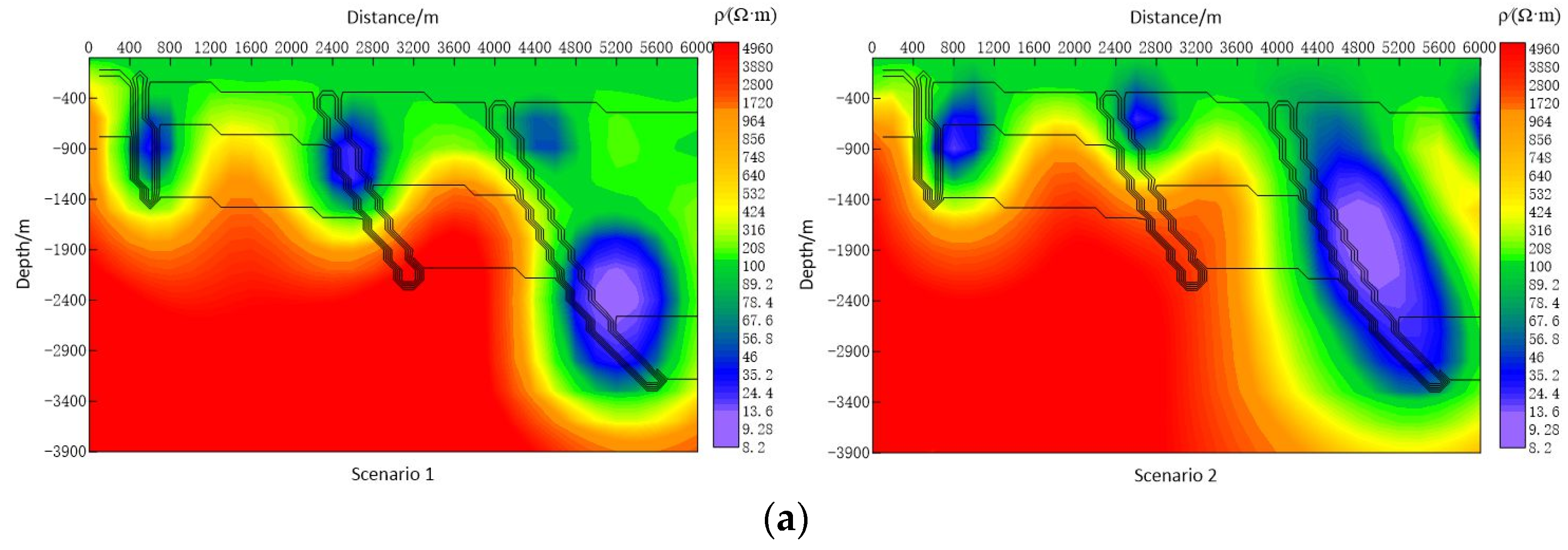
4.1. Effect of Station Spacing on Fault Imaging

The magnetotelluric inversion results (Figure 2a–d) highlight the effect of station spacing on detecting low-resistance fault zones. The station spacings tested range from 200 m to 800 m, and the results consistently show that even at depths of up to 3 km, the linear structure of the faults can be effectively captured. These findings demonstrate the robustness of the employed inversion method across various station spacings, particularly in delineating fault zones spanning shallow to deep subsurface layers.

However, it is evident that smaller station spacings (200 m and 400 m) provide superior accuracy in defining fault geometries and structures compared to larger spacings (600 m and 800 m). In Scenario 1, fault imaging is more precise when the station spacing is reduced to 200 m or 400 m. In these cases, the spatial locations of the three faults, especially F1 and F3, closely align with their actual positions in the geological model, and their depths are well-matched in the inversion results.

In contrast, when the station spacing increases to 600 m or 800 m, the inversion results begin to diverge from the actual fault positions. Notably, the F1 fault exhibits significant positional deviations, suggesting that larger station spacings reduce the reliability of imaging complex fault geometries. This trend is also apparent in Scenario 2, where the 800 m station spacing causes the F3 fault to show a broad influence area with unclear boundaries, indicating a loss of resolution.

Additionally, the F2 fault proves challenging to image across all station spacings and scenarios. Regardless of the acquisition parameters, the inversion consistently fails to accurately resolve the depth and position of the F2 fault, suggesting that this fault may either require a denser dataset or be subject to limitations inherent in the inversion algorithm or the characteristics of the fault zone itself.

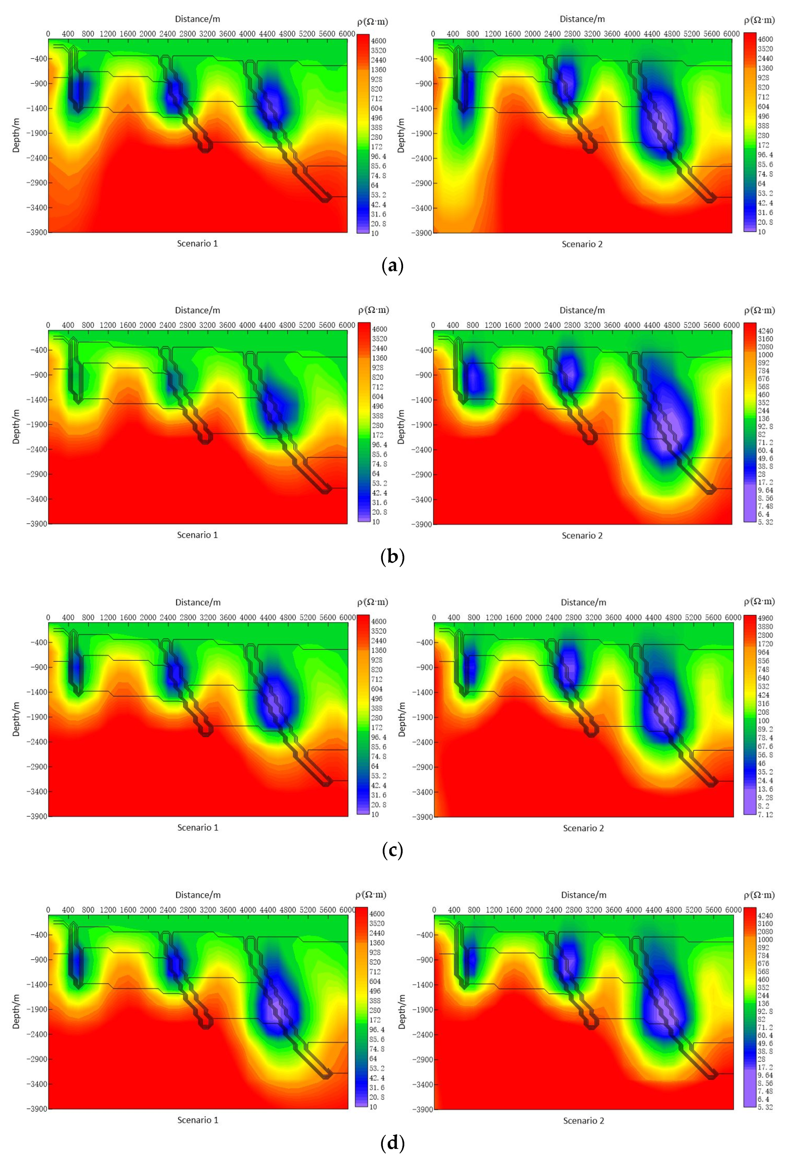
4.2. Effect of Survey Length on Fault Imaging

The inversions (Figure 3a–d) in both scenarios demonstrate that increasing the survey line length enhances the accuracy of fault imaging, particularly for faults F1 and F3. The geological context plays a significant role in these observations, as resistivity contrasts and fault geometries influence the magnetotelluric responses.

In Scenario 2, which features wider faults, the imaging accuracy of F1 improves considerably when the survey line length is extended to 12 km. At this length, the low-resistivity anomalies associated with the F1 fault closely match their true lateral positions in the geological model, and the fault’s localization accuracy surpasses that of Scenario 1. This improvement could be attributed to the wider fault, which allows for better signal penetration and easier detection, even in regions with varying geological conditions.

Interestingly, in Scenario 2, the inversion accuracy of the F3 fault is already high at a survey length of 8 km, with no significant improvements when the length is further increased. This suggests that for wider faults with strong resistivity contrasts, a shorter survey line may be sufficient for accurate imaging. The geological implication here is that fault width and the associated lithological properties can reduce the need for extensive survey lengths in certain cases.

In both scenarios, the imaging accuracy of the F2 fault remains consistently poor, regardless of the survey line length. The inversion depth for F2 is always shallower than the actual depth, resulting in smaller-scale low-resistivity anomalies. This persistent issue may be due to geological factors such as lower resistivity contrast or gradational boundaries between the fault and surrounding rock. These characteristics can weaken the electromagnetic response, making it difficult to accurately image the fault using standard MT inversion techniques. This suggests that additional geological information or advanced inversion methods may be required to resolve such features.

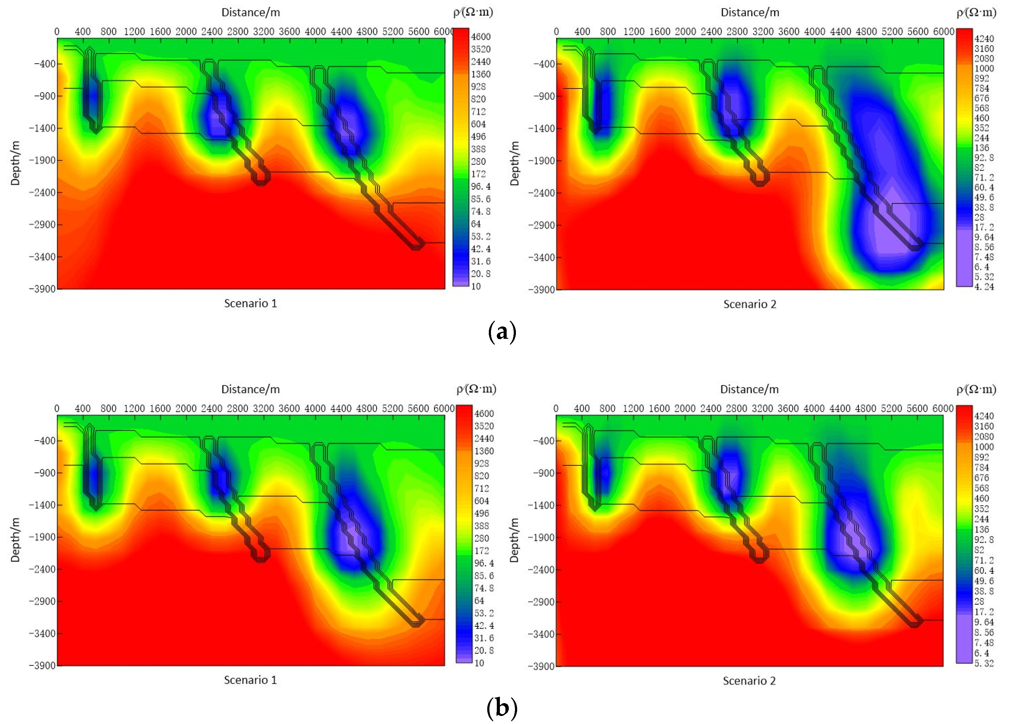
4.3. Effect of Observation Frequency Bands on Fault Imaging

The inversion results (Figure 4a,b) indicate that, in Scenario 1, the fault zone location and resolution from regular inversion bands are inferior to those from broadband survey data, mainly due to the absence of low-frequency data. The inversion depth of the F3 fault is limited to 2 km, failing to fully capture the depth of the fault. This limitation is not observed in any other survey designs discussed in this paper. Additionally, the image area of the F2 and F3 faults appears significantly broader than their actual dimensions, suggesting an overestimation of fault zone width. The fault depth resolution is notably better in Scenario 2 compared to Scenario 1, particularly for the deeper imaging of the F3 fault, which closely matches the broadband survey data. However, the width of the deeper imaging of the F1 and F3 faults is significantly broader than in the geological model, indicating poor resolution of narrow structures. Among all the survey designs, the F2 fault exhibits the poorest imaging quality, with inversion depths significantly diverging from those in the geological model.

5. Conclusions

A geological model containing various fault zones was constructed, and synthetic data was used for forward modeling and inversion to replicate different survey designs. By analyzing how different survey parameters and model grids interpret fault zones in MT detection, we reached the following conclusions:

(1)

Forward modeling results show that a station spacing of 400 m effectively resolves fault zones and transverse conductive fault zones ranging from 100 m to 400 m in width. However, reducing station spacing offers no significant advantage in accurately determining their extent and morphology. In contrast, larger station spacing impacts fault boundary localization and increases deviations from the actual geological model. Specifically, in Scenario 2, when station spacing exceeds 400 m, the imaging of both the F1 and F3 faults deteriorates, with lateral errors increasing from 0.1 km to as much as 1.2 km. These findings emphasize the need for tighter station spacing, particularly in complex geological regions, to achieve accurate fault localization.

(2)

In this study’s geological model, using a 400 m station spacing, a survey length of 12 km or more yields optimal imaging accuracy for fault boundaries (F1 and F3), especially for narrower faults (Scenario 1), enhancing localization accuracy and inversion depth. For wider faults (Scenario 2), increasing the survey length does not significantly improve the clarity of the deeper faults. In both scenarios, the F1 fault is best imaged with a survey length of 12 km, where the lateral error in fault positioning decreases from 1.0 km to less than 0.3 km. For the F3 fault, a 12 km survey reduces its positional error from 1.5 km to 0.2 km. In contrast, the F2 fault consistently shows a shallower inversion depth, with reduced low-resistivity anomalies and an average depth discrepancy of 1.0 km across all survey lengths.

(3)

With a 400 m station spacing, broadband measurements do not significantly improve the clarity of shallow fault structures compared to regular measurements. This limitation may result from insufficient resolution of narrow fault structures in broadband data at a 400 m station spacing. Therefore, acquiring lower frequency and broader bandwidth data through long-period measurements is essential to improve the resolution of deep fault structures.

(4)

The inversion results in this study show a shallower inversion depth compared to the true depth, resulting in poor resolution of the faults’ vertical extent. Additionally, the inversion results suggest that due to the limitations of MT inversion, resistivity models derived from MT data should be interpreted with caution, especially without support from other geophysical methods, as this may affect resource estimation. For instance, the F2 fault zone appears the smallest in the inversion results, with the resistivity model showing the poorest conductivity, contradicting its true characteristics but not diminishing its exploration potential. The forward modeling in this study has been optimized for a two-dimensional observation system, with simplifications made regarding subsurface structures and conductive materials. However, real-world conditions are likely more complex, requiring consideration of factors such as fault connectivity, variations in fault zones across planes, and the types of conductors involved.

References

1. McLeod, J.; Ferguson, I.; Craven, J.; Roberts, B.; Giroux, B. Pre-injection magnetotelluric surveys at the Aquistore CO2 sequestration site, Estevan, Saskatchewan, Canada. Int. J. Greenh. Gas Control 2018, 74, 99–118. [Google Scholar] [CrossRef]
2. Fan, Y.; Chen, X.B.; Tang, J.; Cui, T.F.; Sun, X.Y.; Wang, P.J.; Liu, Z.Y. Three-dimensional modeling of magnetotelluric data from the Hefei-Suqian segment of the Tanlu Fault Zone, Eastern China. Chin. J. Geophys. 2022, 65, 1336–1353. (In Chinese) [Google Scholar]
3. Heinson, G.; Didana, Y.; Soeffky, P.; Thiel, S.; Wise, T. The crustal geophysical signature of a world-class magmatic mineral system. Sci. Rep. 2018, 8, 10608. [Google Scholar] [CrossRef] [PubMed]
4. Jiang, W.P.; Duan, J.M.; Michael, D.; Andrew, C.; Anthony, S.; Brodie, R.C.; Goodwin, J. Application of Multi-Scale Magnetotelluric Data to Mineral Exploration: An Example from the East Tennant Region, Northern Australia. Geophys. J. Int. 2021, 229, 1628–1645. [Google Scholar] [CrossRef] [PubMed]
5. Niu, P.; Han, J.T.; Zeng, Z.F.; Hou, H.S.; Liu, L.J.; Ma, G.Q.; Guan, Y.W. Deep controlling factors of the geothermal field in the northern Songliao basin derived from magnetotelluric survey. Chin. J. Geophys. 2021, 64, 4060–4074. (In Chinese) [Google Scholar]
6. Zhang, J.F.; Sun, N.Q.; Liu, Z.L.; Qi, Z.P. Electromagnetic methods in the detection of water hazards in coal mines: A review. Coal Geol. Explor. 2023, 51, 301–316. [Google Scholar]
7. Nikiforov, V.M.; Varentsov, I.M.; Shkabarnya, G.N.; Kaplun, V.B.; Zhukovin, A.Y.; Cuong, D.H. Long-period (10 < T < 20,000 s) Magnetotelluric Studies in Northern Vietnam. Russ. Geol. Geophys. 2020, 61, 1036–1055. [Google Scholar]
8. He, J.S. Wide field electromagnetic sounding methods. J. Cent. South Univ. (Sci. Technol.) 2010, 41, 1065–1072. [Google Scholar]
9. Cai, J.T.; Chen, X.B.; Fang, L.H.; Qi, H.; Wang, P.J.; Zhang, Y.Y.; Liu, Z.Y.; Xie, X.B.; Zhou, L. Study on the seismotectonic environment in Bengbu city using the dense magnetotelluric array. Chin. J. Geophys. 2023, 66, 638–658. (In Chinese) [Google Scholar]
10. Zhang, J.H.; Zhao, G.Z.; Xiao, Q.B.; Xia, Q.B.; Tang, J. Analysis of electric structure of the central Tan-Lu fault zone (Yi-Shu fault zone, 36°N ) and seismogenic condition. Chin. J. Geophys. 2010, 53, 605–611. (In Chinese) [Google Scholar]
11. Han, J.T.; Kang, J.Q.; Liu, C.; Liu, W.Y.; Zhang, Y.C.; Wang, T.Q.; Guo, Z.Y.; Yuan, T.M.; Liu, L.J. Characteristics of the asthenosphere structure beneath the eastern segment of the Central Asia orogenic belt inferred from a long-period magnetotelluric survey. Chin. J. Geophys. 2019, 62, 1148–1158. (In Chinese) [Google Scholar]
12. Qiao, Y.; Zhang, H. Methodology and Application of Deep Geothermal Sounding in Low-Resistance Cover Areas. Appl. Geophys. 2023; Early Access. [Google Scholar]
13. Zhang, H.; Sui, S.Q.; Qian, L.R. The application of multiple non-seismic methods to geothermal exploration in Qihe Shandong Province. Geophys. Geochem. Explor. 2020, 44, 727–733. [Google Scholar]
14. Patro, P.K. Magnetotelluric Studies for Hydrocarbon and Geothermal Resources: Examples from the Asian Region. Surv. Geophys. 2017, 38, 1005–1041. [Google Scholar] [CrossRef]
15. Geiermann, J.; Schill, E. 2-D Magnetotellurics at the geothermal site at Soultz-sous-Forets: Resistivity distribution to about 3000 m depth. Comptes Rendus Geosci. 2010, 342, 587–599. [Google Scholar] [CrossRef]
16. Pospeeva, E.V.; Potapov, V.V. Deep Structure of the Junction Zones of the Chuya Tectonic Depression and Its Mountainous Frame in Gorny Altai according to Magnetotelluric Studies. Russ. Geol. Geophys. 2021, 62, 474–485. [Google Scholar] [CrossRef]
17. Avdeev, D.B. Three-dimensional electromagnetic modeling and inversion from theory to application. Surv. Geophys. 2005, 26, 767–799. [Google Scholar] [CrossRef]
18. Zhou, R.F.; Wand, X.B.; Qin, C.; Xu, Y.C.; Zhang, J.T.; Wang, R. Comprehensive utilization of NLCG and OCCAM in two-dimensional magnetotelluric inversion. Prog. Geophys. 2016, 31, 2306–2312. [Google Scholar]
19. Chen, M.S. Analysis of some problems on the detecting depth of frequency electromagnetic sounding. Coal Geol. Explor. 2012, 40, 67–70. [Google Scholar]
20. Zhang, H.; Nie, F. Magnetotelluric Forward Modeling Using a Non-Uniform Grid Finite Difference Method. Mathematics 2024, 12, 2984. [Google Scholar] [CrossRef]
21. Gallardo, G.E.U.; Ruiz, A.D. High order edge-based elements for 3D magnetotelluric modeling with unstructured meshes. Comput. Geosci. 2022, 158, 104971. [Google Scholar] [CrossRef]
22. Klaus, S. Electromagnetic Modeling Using Adaptive Grids—Error Estimation and Geometry Representation. Surv. Geophys. 2023, 45, 227–314. [Google Scholar]
23. Tong, X.Z.; Sun, Y.; Zhang, B.Y. An efficient spectral element method for two-dimensional magnetotelluric modeling. Front. Earth Sci. 2023, 11, 1183150. [Google Scholar] [CrossRef]
24. Jahandari, H.; Bihlo, A. Forward modelling of geophysical electromagnetic data on unstructured grids using an adaptive mimetic finite-difference method. Comput. Geosci. 2021, 25, 1083–1104. [Google Scholar] [CrossRef]
25. Erdogan, E.; Candansayar, M.E. The conductivity structure of the Gediz Graben geothermal area extracted from 2D and 3D magnetotelluric inversion: Synthetic and field data applications. Geothermics 2017, 65, 170–179. [Google Scholar] [CrossRef]
26. Zainalpour, A.; Kamali, G.; Moradzadeh, A. Optimal selection of regularization parameter in magnetotelluric data inversion. Acta Geod. Geophys. 2022, 57, 245–263. [Google Scholar] [CrossRef]
27. Wang, P.J.; Chen, X.B.; Zhang, Y.Y. Synthesizing magnetotelluric time series based on forward modeling. Front. Earth Sci. 2023, 11, 1086749. [Google Scholar] [CrossRef]
28. Tomassi, A.; Trippetta, F.; de Franco, R.; Ruggieri, R. How petrophysical properties influence the seismic signature of carbonate fault damage zone: Insights from forward-seismic modelling. J. Struct. Geol. 2023, 167, 104802. [Google Scholar] [CrossRef]
29. Kirkby, A.; Doublier, M.P. Synthetic magnetotelluric modelling of a regional fault network—Implications for survey design and interpretation. Explor. Geophys. 2022, 55, 617–628. [Google Scholar] [CrossRef]
30. Dmitriev, V.I.; Mershchikova, N.A. Mathematical Modeling of the Influence of the Coastal Effect on Marine Magnetotelluric Soundings. Izv.-Phys. Solid Earth 2010, 46, 717–721. [Google Scholar] [CrossRef]
31. Zhang, M.L.; Li, Y.G. Efficient magnetotelluric data acquisition using irregular stations and compressive sensing reconstruction. J. Appl. Geophys. 2023, 217, 105169. [Google Scholar] [CrossRef]
32. Batista, J.D.; Sampaio, E.E.S. Magnetotelluric inversion of one- and two-dimensional synthetic data based on hybrid genetic algorithms. Acta Geophys. 2019, 67, 1365–1377. [Google Scholar] [CrossRef]
33. Arun, S.; Rahul, D.; Pravin, K.G.; Israil, M. A MATLAB based 3D modeling and inversion code for MT data. Comput. Geosci. 2017, 104, 1–11. [Google Scholar]
34. Mackie, R.L.; Smith, J.T.; Madden, T.R. Three-Dimensional electromagnetic modeling using finite-difference equations-the magnetotelluric example. Radio Sci. 1994, 29, 923–935. [Google Scholar] [CrossRef]
35. Rodi, W.; Mackie, R.L. Nonlinear conjugate gradients algorithm for 2D magnetotelluric inversion. Geophysics 2001, 66, 174–187. [Google Scholar] [CrossRef]
36. Kelbert, A.; Egbert, G.D.; Schultz, A. Non-linear conjugate gradient inversion for global em induction: Resolution studies. Geophys. J. Int. 2008, 173, 365–381. [Google Scholar] [CrossRef]
37. Miensopust, M.P.; Queralt, P.; Jones, A.G. Magnetotelluric 3-D inversion- a review of two successful workshops on forward and inversion code testing and comparison. Geophys. J. Int. 2013, 193, 1216–1238. [Google Scholar] [CrossRef]
Figure 1. Geological model depicting three faults (F1, F2, and F3) with varying dip angles and resistivity distribution used for forward modeling.
Applsci 14 09720 g001
Figure 2. Inversion resistivity profile of different station spacings. (a) Station spacing is 200 m. (b) Station spacing is 400 m. (c) Station spacing is 600 m. (d) Station spacing is 800 m.
Applsci 14 09720 g002aApplsci 14 09720 g002b
Figure 3. Inversion resistivity profile of different survey length. (a) Survey length is 8 km. (b) Survey length is 10 km. (c) Survey length is 12 km. (d) Survey length is 14 km.
Applsci 14 09720 g003
Figure 4. Inversion resistivity profile at different observation frequency bands. (a) The observation frequency band is 0.01–100 Hz. (b) The observation frequency band is 0.001–1000 Hz.
Applsci 14 09720 g004