Abstract
Soil thermal conductivity in the near-phase-transition zone is a key parameter affecting the thermal stability of permafrost engineering and its catastrophic thermal processes. Therefore, accurately determining the soil thermal conductivity in this specific temperature zone has important theoretical and engineering significance. In the present work, a method for testing the thermal conductivity of fine sandy soil in the near-phase-transition zone was proposed by measuring thermal conductivity with the transient plane heat source method and determining the volumetric specific heat capacity by weighing unfrozen water contents. The unfrozen water content of sand specimens in the near-phase-transition zone was tested, and a corresponding empirical fitting formula was established. Finally, based on the testing results, temperature variation trends and parameter influence laws of thermal conductivity in the near-phase-transition zone were analyzed, and thermal conductivity prediction models based on multiple regression (MR) and a radial basis function neural network (RBFNN) were also established. The results show the following: (1) The average error of the proposed test method in this work and the reference steady-state heat flow method is only 7.25%, which validates the reliability of the proposed test method. (2) The variation in unfrozen water contents in fine sandy soil in the range of 0~−3 °C accounts for over 80% of the variation in the entire negative temperature range. The unfrozen water content and thermal conductivity curves exhibit a similar trend, and the near-phase-transition zone can be divided into a drastic phase transition zone and a stable phase transition zone. (3) Increases in the thermal conductivity of fine sandy soil mainly occur the drastic phase transition zone, where these increases account for about 60% of the total increase in thermal conductivity in the entire negative temperature region. With the increase in density and total water content, the rate of increase in thermal conductivity in the drastic phase transition zone gradually decreases. (4) The R2, MAE, and RSME of the RBFNN model in the drastic phase transition zone are 0.991, 0.011, and 0.021, respectively, which are better than those of the MR prediction model.
1. Introduction
Over 70% of China’s permafrost is distributed in the Qinghai–Tibet Plateau, which is also the region with the highest altitude and the most extensive permafrost distribution in the middle and low latitudes of the world [1,2,3]. Various large-scale engineering structures widely distributed in the plateau’s permafrost regions significantly affect heat transfer in the soil, ultimately changing the thermal balance and temperature field of the permafrost [4,5,6]. This has led to noticeable permafrost degradation, presenting new problems and challenges to the construction and operation of large-scale linear engineering projects in this region [7,8,9,10]. In terms of practical engineering, the thermal conductivity of permafrost in negative temperature areas, which is close to the initial freezing temperature point (defined as the “near-phase-transition zone”), is the key physical parameter affecting the thermal stability of engineering structures. However, measuring the thermal conductivity of permafrost in the near-phase-transition zone requires temperature control and heat flow monitoring with an extremely high precision, which is limited by cost and complexity. To date, there are no well-established methods for testing the thermal conductivity of permafrost in the near-phase-transition zone, which is crucial for describing the distribution of the permafrost temperature field and ensuring project safety.
Recent investigations into soil thermal conductivity have led to significant progress in various aspects. Researchers have carried out a large number of studies on thermal conductivity test methods. For instance, Xu et al. [11] utilized the calorimeter method, the heat flow meter method, and the probe method to measure the thermal conductivity of various frozen soils and established a series of widely used thermal parameter tables for frozen soil. Nusier et al. [12] conducted laboratory testing using single- and dual-probe methods to determine the thermal conductivity of loam and found that the test results of the dual-probe method were more accurate than those of the single-probe method. Lu et al. [13] and Zhang et al. [14] also carried out a series of experimental studies on the thermal conductivity of aeolian sandy soil, clay, and silty clay using the transient hot wire method. With advancements in theoretical understanding and technological capabilities, numerous scholars have further improved and proposed new thermal conductivity testing techniques. For example, Alrtimi et al. [15] incorporated a heat jacket into the frozen soil thermal conductivity testing apparatus used in the steady-state comparative method, significantly reducing the radial heat loss of the device and enhancing measurement accuracy. Kojima et al. [16] designed an innovative dual-probe thermal pulse sensor for the measurement of the thermal properties of frozen soil.
To avoid costly and time-consuming experimental procedures and to facilitate engineering applications, researchers have conducted statistical analyses on a large amount of frozen soil thermal conductivity test data and proposed many data-driven empirical formulas [17,18]. Based on the results of testing 19 soil types, Kersten [19] established initial empirical formulas for thermal conductivity using water content and dry density. Johansen [20] proposed an interpolation calculation model of soil thermal conductivity using normalized coefficients and soil saturation. Bi et al. [21] developed a general model for calculating the thermal conductivity of frozen soil which is based on the liquid water content, frost heave, porosity, and initial water content. Tian et al. [22] established an empirical model of the relationship between thermal conductivity and porosity based on data from 28 partially frozen soils. Scholars have also made many improvements to classic thermal conductivity empirical models to broaden their applicability and increase their prediction accuracy. For example, He et al. [23] established a new model similar to the Johansen model which simulates the relationship between various soil textures and their water contents and effective thermal conductivities. Zeng et al. [24] compared and evaluated eight soil thermal conductivity models through actual measurements and proposed an improved thermal conductivity prediction model that considers particle size distribution parameters. Balland et al. [25] expanded Johansen’s model and developed a thermal conductivity calculation model that is applicable to more soil conditions. Compared with traditional empirical fitting methods, machine learning methods can achieve more accurate estimations through training with a large amount of data, and they have also been widely used for the prediction of frozen soil thermal conductivity [26,27,28]. For instance, Ren et al. [29] analyzed the factors affecting the thermal conductivity of soil during the freeze–thaw process and established a prediction model for thermal conductivity using artificial neural network technology. Kardani et al. [30] combined the firefly algorithm with the extreme learning machine method to establish a model for predicting the thermal conductivity of unsaturated soil.
In recent years, researchers have also studied measurement methods and predictive models of the soil thermal conductivity in the near-phase-transition zone. For example, Zhao et al. [31] combined the steady-state method with the transient method and proposed a method for measuring the thermal conductivity of frozen soil near 0 °C. After an analysis of various models for estimating characteristic soil freezing curves, Bi et al. [32] proposed a new method for predicting the thermal conductivity of frozen soil based on the geometric mean model. This model can effectively predict the thermal conductivity of frozen soil and how it varies in the temperature range of −20 °C to 0 °C. He et al. [33] used the steady-state method to measure the thermal conductivity of frozen and thawed lime soil and found that the phase change in the soil mainly occurs between −3 and −2 °C. Firat et al. [34,35] proposed an artificial neural network prediction model based on the internal and external factors of the soil, which can effectively predict the thermal conductivity of sandy soil at temperatures ranging from −7 °C to 4 °C. Although extensive research has been conducted on the thermal conductivity of various types of frozen soil [36], studies on the thermal conductivity characteristics of frozen soil in the near-phase-transition zone are relatively scarce. Existing thermal conductivity data of frozen soil were mostly measured at low temperatures (e.g., T < −4 °C), and there is a lack of test data near the phase change point [37,38]. Furthermore, current models for predicting the thermal conductivity of frozen soil in the near-phase-transition zone have limitations in terms of accuracy and applicability [39,40]. To address this, in the present work, a method for testing the thermal conductivity of fine sandy soil in the near-phase-transition zone is proposed. This method involves measuring thermal conductivity using the transient plane heat source method and determining the volumetric specific heat capacity via weighing the unfrozen water content. The unfrozen water content of sand specimens in the near-phase-transition zone was determined using nuclear magnetic resonance (NMR) technology, and corresponding empirical fitting formulas were established. Based on the test results, the temperature variation characteristics and parameter influence laws of thermal conductivity in the near-phase-transition zone were investigated. Additionally, thermal conductivity prediction models based on multiple regression (MR) and a radial basis function neural network (RBFNN) were established.
2. Materials and Methods
2.1. Source of Experimental Soil Specimens
Experimental specimens were obtained via the drilling sampling method, with sampling locations located between Xidatan and Tanggula mountain along the Qinghai–Tibet Engineering Corridor (the corresponding mileage of the Qinghai–Tibet Highway is K2881~K3307, as shown in Figure 1). This is the main permafrost area on the northern edge of the Qinghai–Tibet Plateau. The total number of specimens was 124, and the sampling depth was 0.5~36.5 m.
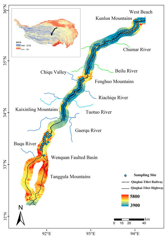
Figure 1.
Schematic of the sampling spots for soil specimens.
The particle size (s) distribution was determined using a Bettersize2000 laser particle size distribution instrument, and the results are shown in Figure 1; the soil specimen corresponding to these results was taken from a section of the Qingshuihe River (Figure 2). The particle size distribution range of the test samples was 0.345~633.6 μm, with the particle size mainly distributed (cumulative distribution probability 20%~80%) in the range of 92.01~267 μm. The proportion of clay (s < 0.005 mm), silt (0.005 mm ≤ s < 0.075 mm), and sand (s > 0.075 mm) was 5.13%, 9.03%, and 85.54%, respectively. The specimen’s volume-weighted average diameter and specific surface area were 0.198 mm and 0.101 m2/g, respectively. Based on the classification standard of the Geotechnical Engineering Investigation Code (GB 50021−2001) [41], the experimental soil specimens in the present work were classified as fine sandy soil.

Figure 2.
Particle size distribution of the fine sandy soil specimens.
The specimens used for experiments were remolded soil samples. According to the data from the 124 fine sandy soil specimens, the average water content and density were 16.9% and 2.03 g/cm3, respectively, with these values mainly distributed within (cumulative distribution probability of 20~80%) 10.4~20% and 1.9~2.18 g/cm3, respectively. Considering sample preparation and the testing time, we selected 51 groups of sandy soil specimens from typical sections along the Qinghai–Tibet Engineering Corridor for testing; the basic physical properties of the tested soil specimens are listed in Table 1.

Table 1.
Basic physical properties of the tested soil specimens.
2.2. Method of Measuring Thermal Conductivity of Sandy Soil in the Near-Phase-Transition Zone
In this study, the thermal conductivity of sandy soil specimens in the near-phase-transition zone was calculated using the test results of thermal diffusivity and specific heat capacity:
where λ is the thermal conductivity of a sandy soil specimen, α is its thermal diffusivity, and C is its volumetric specific heat capacity.
The thermal diffusivity was measured using the transient plane source method. The experimental system consisted of a Hot Disk TPS1500s Thermal Conductivity Analyzer, a high-precision environmental cabinet and a data acquisition system, as shown in Figure 3. According to geotechnical testing standards, the remolded testing soil specimens were fabricated using the hydraulic press demudding method. In order to improve the test accuracy, cylindrical specimens with a diameter of 80 mm and a height of 30 mm and a circular Kapton sensor with a diameter of 29.4 mm were adopted. The testing temperatures were divided into two ranges, positive temperatures and negative temperatures, in which the controlling temperature of the positive temperature range was 10 °C. The negative temperature range was defined from initial freezing temperature point of the tested sample (Tf) to −15 °C. Since the initial freezing temperatures of the tested soil specimens were all around −0.5 °C, the starting point of the negative temperature range was set to −0.5 °C to simplify the experimental protocol and facilitate analysis. Furthermore, in order to more accurately capture the trends in thermal diffusivity of the tested samples in the near-phase-transition zone, an experimental strategy using small temperature intervals was applied in this temperature range. The specific test temperature points were −15 °C, −11 °C, −8 °C, −6 °C, −4 °C, −3 °C, −2 °C, −1.5 °C, −1 °C, −0.7 °C, and −0.5 °C.

Figure 3.
Thermal diffusivity testing instrument.
The volumetric specific heat capacity was calculated using the theoretical calculation method [10]. In this calculation method, it is assumed that the soil’s volumetric specific heat capacity is the mass-weighted average of its multiphase components, including the soil skeleton, water and ice. The calculation formula is as follows:
where Cu and Cf are the volumetric specific heat capacity of unfrozen and frozen soil samples, respectively; Csu, Csf, Cw and Ci are the mass specific heat capacity of unfrozen soil skeleton, frozen soil skeleton, water, and ice, respectively, for which specific values are listed in Table 2; ρu and ρf are the natural density of unfrozen soil and frozen soil, respectively; and W0 and Wu are total water content and unfrozen water content, respectively.
Table 2.
Specific values of mass specific heat capacity of soil components.
Given that the density (ρu and ρf) and total water content (W) of the specimen are known, its volumetric specific heat capacity in the near-phase-transition zone can be obtained by determining the unfrozen water content at different temperatures. In the present work, NMR was used to determine the unfrozen water content of soil specimens in the near-phase-transition zone. A low-temperature and high-pressure MesoMR NMR analyzer (Niumag, Suzhou, China) was used for NMR analysis, which is composed of a permanent magnet, a radio frequency unit and a data acquisition system (Figure 4). A B2220 high-precision cryogenic circulating bath (Xiatech, Xi’an, China) was utilized to cool the specimen to the specified temperature. The parameters of the NMR testing system are listed in Table 3.

Figure 4.
Schematic of the NMR experimental procedure and system.
Table 3.
Parameters of the NMR testing system.
The geometric dimensions of the specimen, as determined via NMR, were 38.1 mm (diameter) and 100 mm (height). To ensure a uniform soil specimen temperature, the sand bath method was used to cool the sample to the required temperature. Considering the drastic changes in unfrozen water content in the near-phase-transition zone, the temperature testing points for NMR were consistent with those used to measure the thermal diffusivity. The formula for calculating unfrozen water contents using NMR measurements is as follows:
where Ai is the NMR signal intensity value at a certain negative temperature point and Aj is the NMR signal intensity corresponding to the paramagnetic regression line at the current temperature. The paramagnetic regression line was obtained via NMR signal fitting at positive temperatures of 20 °C, 15 °C, 10 °C and 5 °C.
2.3. Method of Predicitng Thermal Conductivity of Sandy Soil in the Near-Phase-Transition Zone
Previous investigations have shown that indicators such as excess temperature (), unfrozen soil thermal conductivity (), and completely frozen soil thermal conductivity () have a significant influence on the soil’s thermal conductivity in the near-phase-transition zone () [42]. A partial correlation analysis of the above factors was performed, and the results are shown in Table 4. The results show that the thermal conductivity of the sand sample had certain correlations with , and both in the drastic and stable phase transition zones (see Section 3.1 for details). The partial correlation coefficients between and , and were −0.772, 0.228 and 0.934 in the stable phase transition zone, and −0.685, 0.462, 0.912 in the drastic phase transition zone, respectively. Furthermore, the significance coefficients were all less than 0.01, which indicates that the above three factors can be used to predict the soil’s thermal conductivity in the near-phase-transition zone.
Table 4.
Partial correlation analysis between and , and .
The multivariate regression (MR) fitting method was used to predict the soil’s thermal conductivity in the near-phase-transition zone. The unfrozen water content and thermal conductivity in frozen soil in the near-phase-transition zone changed drastically close to the phase transition temperature and were stable at low temperatures. Thus, the MR fitting formula for the thermal conductivity of frozen soil in the near-phase-transition zone was set as a piecewise function of temperature, namely stable and drastic phase transition zones. In order to select an appropriate multivariate regression function, fitting of the curve between and the above three factors was performed. It was found that the soil thermal conductivity in the stable phase transition zone was linearly related to these three factors, while in the drastic phase transition zone, the thermal conductivity was linearly related to the frozen and unfrozen soil thermal conductivities and exponentially related to the excess temperature. The MR prediction formulas of are as follows:
where is the soil thermal conductivity in the near-phase-transition zone; is the excess temperature, which is calculated according to ; is the unfrozen soil thermal conductivity; is the frozen soil thermal conductivity; and a, b, c and d are all fitting coefficients.
The RBFNN model was adopted in this work due to its strong local approximation, fast learning convergence speed, low computational burden and extensive generalization ability in order to establish a soil thermal conductivity prediction model in the near-phase-transition zone [43,44]. The RBFNN model has a three-layer structure, involving an input layer, a hidden layer and an output layer. Considering the relatively small amount of sampling data, the K-fold cross-validation method was applied to obtain the optimal model. The following Gaussian kernel function was used as the activation function in the RBFNN model:
where xp is the input unit; ci is the central vector; and σ is the width parameter of the function.
The least squares method was chosen as the loss function formula:
where p is the number of input samples; dj is the expected output value; and yj is the output unit.
Similarly, the factors of , and were selected as the predictors of the input layer nodes of the RBFNN model. (for drastic and stable phase transition zones) was set as the output layer, and the hidden layer was assigned a two-layer structure, with 13 nodes in the first layer and 10 nodes in the second layer. We compared the prediction accuracy of the RBFNN model with different combinations of node numbers in each hidden layer, and finally determined that the ideal number of nodes was 13 for the first layer and 10 for the second layer. Then, all of the test results were randomly divided into a 7:3 ratio, with 70% of the test data used for training samples and the remaining 30% used to validate the RBFNN predictive model. A schematic diagram of RBFNN model’s structure is shown in Figure 5.
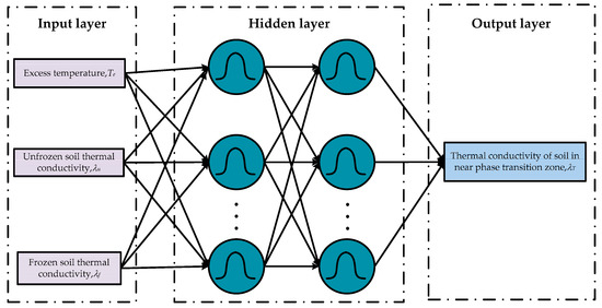
Figure 5.
Structure of the RBFNN model.
To analyze the accuracy of the MR and RBFNN prediction models, three statistical indexes, namely the mean absolute error (MAE), root mean square error (RMSE), and determination coefficient (R2), were used as evaluation indicators. The calculation formulas for R2, MAE and RMSE are given as follows:
where is the predicted value; is the measured value; and is the average value.
2.4. Testing Method Validation
In order to validate the reliability of the testing method, a comparison of soil thermal conductivities determined via the transient method developed in present work and the steady-state heat flow method in ref. [42] was conducted. Figure 6 shows the results of the transient and steady-state methods for positive and negative temperature ranges. Although the values predicted by the proposed method are slightly lower than those of the steady-state method, it can be seen that they exhibit similar trends, and the relative error of the two methods is roughly less than 10%.

Figure 6.
Comparison of soil thermal conductivities predicted by the transient method developed in the present work and those predicted by the steady-state heat flow method in ref. [42]: (a) room temperature; (b) near-phase-transition zone.
Table 5 shows a comparison of the errors of the test methods in the present work and in ref. [42] for different dry densities and water contents. It can be observed that the error in frozen soil thermal conductivity is between 4.93% and 10.13%, while the error for thawed soil is between 2.09% and 7.83%. The results of this work are in good agreement with those in the literature. In addition, it is noted that the average test error gradually decreases with an increase in water content and dry density. Considering that the dry density and water content of sandy soil samples in the Qinghai–Tibet Engineering Corridor are usually high, the errors of our method and the method from the literature will be further reduced. To summarize, the test method in the present work has been validated as a reliable method for measuring the thermal conductivity of frozen soil in the near-phase-transition zone.
Table 5.
Comparison of errors of the method developed in the present work and the method in ref. [42].
3. Results and Discussion
3.1. Trends in Sandy Soil Thermal Conductivity in the Near-Phase-Transition Zone
Based on the proposed testing method, the thermal conductivity of sandy soil specimens in the near-phase-transition zone was obtained and analyzed. The natural density of the sandy soil samples tested in this study ranged from 1.83 to 2.39 g/cm3, with an average of 2.05 g/cm3, and the water content range was 7.3%~28.3%, with an average of 13.9%. According to the classification standard of frozen soil [45], the test soil samples were divided into four types, namely ice-poor (W0 ≤ 12%), icy (12 < W0 ≤ 18%), ice-rich (18 < W0 ≤ 25%), and ice-saturated (W0 > 25%) frozen soil.
Figure 7 shows the variation in thermal conductivity of different soil types in the negative temperature range. It can be seen that, as the temperature decreases, the thermal conductivity of sandy soil specimens decreases. When the temperature is far away from the phase transition point (e.g., >−4 °C), the soil thermal conductivity remains relatively stable and resistant to temperature changes. When approaching the phase transition temperature point (e.g., <−2 °C), the soil thermal conductivity changes dramatically with temperature, and the magnitude of the change rapidly increases as the temperature approaches the phase change point. This is because, when the temperature drops, the unfrozen water in the soil sample transforms from liquid to solid. The volume of ice is 1.1 times that of water, and the increased amount of ice fills the pores inside the soil sample, thereby increasing the contact area for heat transfer. The solid ice also enhances the thermal conductivity of the soil itself (the thermal conductivity of ice is four times that of water). Therefore, the soil thermal conductivity significantly increases as the temperature decreases, especially in the near-phase-transition zone where the liquid water undergoes considerable changes.

Figure 7.
Variation in thermal conductivity of different soil types in the negative temperature range: (a) ice-poor frozen soil; (b) icy frozen soil; (c) ice-rich frozen soil; (d) ice-saturated frozen soil.
It can also be observed that the thermal conductivity of the soil specimens increases as the dry density increases. In addition, the thermal conductivity increase caused by the increase in dry density is greater for ice-poor and icy frozen soils, but relatively insignificant for ice-rich and ice-saturated frozen soils. As shown in Figure 7, when the dry density increases from 1.79 to 1.95 g/cm3 (Figure 7a) and from 1.72 to 2.02 g/cm3 (Figure 7b), the thermal conductivity of completely frozen soil increases by 0.402 W/(m·°C) and 1.277 W/(m·°C), respectively, whereas when the dry density increases from 1.66 to 2.08 g/cm3 (Figure 7c), the thermal conductivity of the soil specimen only increases by 0.063 W/(m·°C). Furthermore, it was observed that the water content has a great effect on the extent of the increase in sandy soil thermal conductivity in the near-phase-transition zone. The higher the water content, the lower the temperature at which the thermal conductivity of the soil tends to stabilize.
3.2. Near-Phase-Transition Zone Delineation Based on NMR Testing Results
The drastic change in unfrozen water content is a key reason for the intense variation in soil thermal conductivity in the near-phase-transition zone [46]. To reveal the temperature variation trends in unfrozen water in sandy soil, 10 groups of specimens were tested using NMR. The dry density of specimens varied from 1.86 g/cm3 to 2.18 g/cm3, with an average of 2.06 g/cm3, and the water content range was 9.2%~21.3%, with an average of 14%.
Figure 8 shows the measurement results of unfrozen water in sand specimens at different temperatures. It can be seen that the unfrozen water content in sand specimens changes drastically at temperatures around the near-phase-transition point. In this range, spanning about 3 °C, the unfrozen water content decreases from 15.5% of the initial water content to 2.9% (light red area in Figure 8). Considering the huge reduction in the proportion of unfrozen water, the soil thermal conductivity will change greatly in this narrow temperature range, so we define this temperature interval as the drastic phase transition zone. Conversely, at temperatures away from the phase transition point (light blue area in Figure 8), the proportion of unfrozen water is only 18.7% of the initial water content; thereby, it is defined as a stable phase transition zone.

Figure 8.
Test results of unfrozen water of sand specimen at different temperatures.
The relationship between unfrozen water content and temperature (T) was fitted using the following formula:
where and are the fitting parameters.
Table 6 shows the results of fitting the relationship between the unfrozen water content and the temperature of the testing samples. It can be seen that the R2 of each sample is above 0.9, indicating the formula fits well. Furthermore, in order to determine the temperature limit (Tlimit) of the drastic and stable phase transition zones, the slope at every temperature measurement point on the fitted curve was calculated. The temperature corresponding to the average slope was used as the temperature limit of the near phase and stable phase transition regions. As shown in Table 6, the range of Tlimit is −3.24~−4.04 °C, and its average value is −3.5 °C. Accounting for the rate of change in unfrozen water content can synchronously reflect the trends in soil thermal conductivity. Thus, in this work, the average temperature limit of unfrozen water was used as Tlimit to analyze the thermal conductivity in the near-phase-transition zone.
Table 6.
Fitting results of the unfrozen water content and temperature of the test samples.
3.3. Prediction Model of Thermal Conductivity of Fine Sandy Soil in the Near-Phase-Transition Zone
To improve the model’s prediction accuracy, multivariate regression fitting formulas for the thermal conductivity in the drastic and stable phase transition zones were established. The MR prediction formulas are as follows:
Figure 9 exhibits the prediction results of the MR model in different temperature ranges. It shows that the predictions of the MR model are in good agreement with the experimental values, with most of the sampling points distributed within ±10% error, which proves the model’s effectiveness and value for engineering application. However, it is worth noting that the prediction results in the drastic phase transition zone still have a certain degree of error; some predicted values deviate from the experimental values by more than 50%. This is attributed to the highly nonlinear characteristics of thermal conductivity in this temperature interval.

Figure 9.
Prediction results of the MR model: (a) drastic phase transition zone; (b) stable phase transition zone.
A comparison of the values predicted by the RBFNN model with the experimental results is given in Figure 10. It can be seen that the prediction accuracy of the RBFNN model is better than that of the MR model. All prediction points are distributed within the ±10% error lines. Moreover, the RBFNN model has a better performance in the drastic phase transition temperature zone. The largest prediction error is only 8.69%, which further demonstrates the superiority of this machine learning method over traditional formula fitting methods.

Figure 10.
Prediction results of the RBFNN model: (a) drastic phase transition zone; (b) stable phase transition zone.
Table 7 shows a comparison of the mean absolute error (MAE), root mean square error (RMSE), determination coefficient (R2), and proportion of error within ±10% () of different thermal conductivity prediction models. It can be seen that both prediction models have a high accuracy, with all the values above 90%. The R2 of the RBFNN model in drastic and stable phase transition zones is 0.991 and 0.986, respectively, while the R2 of the MR model is 0.82 and 0.97, respectively. In addition, the MAE and RSME of the RBFNN model in drastic and stable phase transition zones are 0.011, 0.021, 0.022, and 0.038, respectively, while those of the MR model are much higher, reaching 0.079, 0.166, 0.037, and 0.049, respectively. It can be inferred that the prediction effect of the RBFNN model is better than that of the MR model, proving that the RBFNN model can more effectively capture and replicate the relationship between conductivity and predictors.
Table 7.
Comparison of the prediction effect of MR and RBFNN models.
4. Conclusions
In the present work, a method of determining the thermal conductivity of sandy soils in the near-phase-transition zone was proposed, and the temperature variation trends and parameter influence laws of thermal conductivity were investigated. Moreover, prediction models based on MR and RBFNN methods were established, and the prediction accuracies of the different models were compared. The conclusions are as follows:
- (1)
- The average error between the proposed method and the steady-state heat flow method for soil thermal conductivity in the near-phase-transition zone is 7.25% and the maximum error is 10.1%, which verifies the reliability of the proposed test method.
- (2)
- The unfrozen water content in fine sandy soil changes drastically in the near-phase-transition zone, and the amplitude of this change in the range of 0~−3 °C accounts for over 80% of the total change in the entire negative temperature range. The changes in unfrozen water content and thermal conductivity in fine sandy soil exhibit similar trends, and the near-phase-transition zone temperature interval can be divided into a drastic phase transition zone and a stable phase transition zone.
- (3)
- Increases in the thermal conductivity of fine sandy soil mainly occur in the drastic phase transition zone; these increases account for about 60% of the total increase in thermal conductivity across the entire negative temperature region. With the increase in density and total water content, the rate of the increase in thermal conductivity in the drastic phase transition zone gradually decreases.
- (4)
- The prediction models based on the MR and RBFNN methods both have a high accuracy, which highlights their engineering application value. The R2, MAE, and RSME of the RBFNN model in the drastic phase transition zone are 0.991, 0.011, and 0.021, respectively, and are better than those of the MR prediction model.
This study can help researchers to understand trends in the thermal conductivity of sandy soils with temperature in the near-phase-transition zone and also provides basic thermal data for the design of the future Qinghai–Tibet expressway. However, it should be noted that the MR fitting formula of thermal conductivity in the near-phase-transition zone is only applicable to fine sandy soil, and when the dry density of the sample is relatively small, there may be large errors in the predicted values in the drastic phase transition zone. In addition, although the RBFNN prediction model has a high accuracy in both the drastic and stable phase transition zones, it is naturally a data-driven method and its prediction accuracy depends on the amount of test data; thus, a certain amount of data are required for engineering designers to utilize it.
Author Contributions
Conceptualization, J.L. and Y.Z. (Yue Zhai); methodology, J.L. and P.L.; software, H.H. and L.T.; validation, J.L., Z.L. and Y.Z. (Yue Zhai); formal analysis, P.L. and Y.Z. (Yaxing Zhang); investigation, J.L. and P.L.; resources, Z.L. and Y.Z. (Yue Zhai); data curation, J.L. and Y.Z. (Yue Zhai); writing—original draft preparation, J.L.; writing—review and editing, J.L. and Y.Z. (Yue Zhai). All authors have read and agreed to the published version of the manuscript.
Funding
This research was funded by the National Science Foundation of China (Grant Nos. 42371149, 42230712), the open fund of National Key Laboratory of Green and Long-Life Road Engineering in Extreme Environment (YGY2021KFKT03), and the Scientific Innovation Practice Project of Postgraduates of Chang’an University (300103723048). We are grateful to the anonymous reviewers for their constructive comments to improve this manuscript.
Institutional Review Board Statement
Not applicable.
Informed Consent Statement
Not applicable.
Data Availability Statement
The data presented in this study are available on request from the corresponding author.
Conflicts of Interest
The authors declare no conflicts of interest.
Abbreviations
| Nomenclature | |
| MAE | Mean absoluteError |
| MR | Multiple regression |
| NMR | Nuclear magnetic resonance |
| R2 | Determination coefficient |
| RBFNN | Radial basis function neural network |
| RMSE | Root mean square error |
| Symbols | |
| Ai | NMR signal intensity value at a certain negative temperature point |
| Aj | NMR signal intensity value given by paramagnetic regression |
| a, b, c, d | Fitting coefficients |
| Cu | Volumetric specific heat capacity of unfrozen soil sample |
| Cf | Volumetric specific heat capacity of frozen soil sample |
| Csu | Mass specific heat capacity of unfrozen soil skeleton |
| Csf | Mass specific heat capacity of frozen soil skeleton |
| Cw | Mass specific heat capacity of water |
| Ci | Mass specific heat capacity of ice |
| P | Partial correlation coefficient |
| Excess temperature | |
| Freezing temperature | |
| W0 | Total water content |
| Wu | Unfrozen water content |
| α | Thermal diffusivity |
| ρu | Natural density of unfrozen soil |
| ρf | Natural density of frozen soil |
| λ | Thermal conductivity |
| Soil thermal conductivity in near-phase-transition zone | |
| Unfrozen soil thermal conductivity | |
| Frozen soil thermal conductivity |
References
- Qin, D.H. Introduction to Cryosphere Science; Science Press: Beijing, China, 2018; pp. 35–37. [Google Scholar]
- Luo, Y.; Qin, D.; Zhai, P.; Ma, L.; Zhou, B.; Xu, X. Cryospheric Climatology: Emerging Branch of Cryospheric Science. Bull. Chin. Acad. Sci. 2020, 35, 407–413. [Google Scholar]
- Chang, J.; Ye, R.; Wang, G. Review: Progress in permafrost hydrogeology in China. Hydrogeol. J. 2018, 26, 1387–1399. [Google Scholar] [CrossRef]
- Zheng, X.; Wang, Y.; Zhang, S.; Xu, F.; Zhu, X.; Jiang, X.; Zhou, L.; Shen, Y.; Chen, Q.; Yan, Z.; et al. Research progress of the thermophysical and mechanical properties of concrete subjected to freeze-thaw cycles. Constr. Build. Mater. 2022, 330, 127254. [Google Scholar] [CrossRef]
- Wu, Q.; Sheng, Y.; Yu, Q.; Chen, J.; Ma, W. Engineering in the rugged permafrost terrain on the roof of the world under a warming climate. Permafr. Periglac. Process. 2020, 31, 417–428. [Google Scholar] [CrossRef]
- Ren, X.; Niu, F.; Yu, Q.; Yin, G. Research progress of soil thermal conductivity and its predictive models. Cold Reg. Sci. Technol. 2024, 217, 104027. [Google Scholar]
- Huang, Y.; Niu, F.; Chen, J.; He, P.; Yuan, K.; Su, W. Express highway embankment distress and occurring probability in permafrost regions on the Qinghai-Tibet Plateau. Transp. Geotech. 2023, 42, 101069. [Google Scholar] [CrossRef]
- Jiao, C.; Wang, Y.; Shan, Y.; He, P.; He, J. Quantifying the effect of a retrogressive thaw slump on soil freeze-thaw erosion in permafrost regions on the Qinghai-Tibet Plateau. China. Land Degrad. Dev. 2023, 34, 2573–2588. [Google Scholar] [CrossRef]
- Chen, Z.; Li, Y.; Lai, Y.; Su, C. Non-stationary random vibration analysis of railway embankments in permafrost regions under train loads using the explicit time-domain method. J. Glaciol. Geocryol. 2022, 44, 555–565. [Google Scholar]
- Yu, W.; Zhang, T.; Lu, Y.; Han, F.; Zhou, Y. Engineering risk analysis in cold regions: State of the art and perspectives. Cold Reg. Sci. Technol. 2020, 171, 102963. [Google Scholar] [CrossRef]
- Xu, X.; Wang, J.; Zhang, L. Physics of Frozen Soil; Science Press: Beijing, China, 2001. [Google Scholar]
- Nusier, O.; Abu-Hamdeh, N. Laboratory techniques to evaluate thermal conductivity for some soils. Heat Mass Transf. 2003, 39, 119–123. [Google Scholar] [CrossRef]
- Lu, Y.; Yu, W.; Hu, D.; Liu, W. Experimental study on the thermal conductivity of aeolian sand from the Tibetan Plateau. Cold Reg. Sci. Technol. 2018, 146, 1–8. [Google Scholar] [CrossRef]
- Zhang, M.; Lu, J.; Lai, Y.; Zhang, X. Variation of the thermal conductivity of a silty clay during a freezing-thawing process. Int. J. Heat Mass Transfer. 2018, 124, 1059–1067. [Google Scholar] [CrossRef]
- Alrtimi, A.; Rouainia, M.; Manning, D.A.C. An improved steady-state apparatus for measuring thermal conductivity of soils. Int. J. Heat Mass Transf. 2014, 72, 630–636. [Google Scholar] [CrossRef]
- Kojima, Y.; Heitman, J.L.; Noborio, K.; Ren, T.; Horton, R. Sensitivity analysis of temperature changes for determining thermal properties of partially frozen soil with a dual probe heat pulse sensor. Cold Reg. Sci. Technol. 2018, 151, 188–195. [Google Scholar] [CrossRef]
- Du, Y.; Li, R.; Zhao, L.; Yang, C.; Wu, T.; Hu, G.; Xiao, Y.; Zhu, X.; Yang, S.; Ni, J.; et al. Evaluation of 11 soil thermal conductivity schemes for the permafrost region of the central Qinghai-Tibet Plateau. Catena 2020, 193, 104608. [Google Scholar] [CrossRef]
- Zhang, N.; Wang, Z.Y. Review of soil thermal conductivity and predictive models. Int. J. Therm. Sci. 2017, 117, 172–183. [Google Scholar] [CrossRef]
- Kersten, M.S. Laboratory Research for the Determination of the Thermal Properties of Soils; University of Minnesota: Minneapolis, MN, USA, 1949. [Google Scholar]
- Johansen, O. Thermal Conductivity of Soils; Trondheim University: Trondheim, Norway, 1975. [Google Scholar]
- Bi, J.; Zhang, M.; Lai, Y.; Pei, W.; Lu, J.; You, Z.; Li, D. A generalized model for calculating the thermal conductivity of freezing soils based on soil components and frost heave. Int. J. Heat Mass Transf. 2020, 150, 119166. [Google Scholar] [CrossRef]
- Tian, Z.; Ren, T.; Heitman, J.L.; Horton, R. Estimating thermal conductivity of frozen soils from air-filled porosity. Soil Sci. Soc. Am. J. 2020, 84, 1650–1657. [Google Scholar] [CrossRef]
- He, H.; Zhao, Y.; Dyck, M.F.; Si, B.; Jin, H.; Lv, J.; Wang, J. A modified normalized model for predicting effective soil thermal conductivity. Acta Geotech. 2017, 12, 1281–1300. [Google Scholar] [CrossRef]
- Zeng, S.; Yan, Z.; Yang, J. An improved model for predicting the thermal conductivity of sand based on a grain size distribution parameter. Int. J. Heat Mass Transf. 2023, 207, 124021. [Google Scholar] [CrossRef]
- Balland, V.; Arp, P.A. Modeling soil thermal conductivities over a wide range of conditions. J. Environ. Eng. Sci. 2005, 4, 549–558. [Google Scholar] [CrossRef]
- Zhang, T.; Wang, C.J.; Liu, S.Y.; Zhang, N.; Zhang, T.W. Assessment of soil thermal conduction using artificial neural network models. Cold Reg. Sci. Technol. 2020, 169, 102907. [Google Scholar] [CrossRef]
- Li, K.Q.; Liu, Y.; Kang, Q. Estimating the thermal conductivity of soils using six machine learning algorithms. Int. Commun. Heat Mass Transf. 2022, 136, 106139. [Google Scholar] [CrossRef]
- Zhao, T.; Liu, S.; Xu, J.; He, H.; Wang, D.; Horton, R.; Liu, G. Comparative analysis of seven machine learning algorithms and five empirical models to estimate soil thermal conductivity. Agric. For. Meteorol. 2022, 323, 109080. [Google Scholar] [CrossRef]
- Ren, X.; You, Y.; Yu, Q.; Zhang, G. Determining the thermal conductivity of clay during the freezing process by artificial neural network. Adv. Mater. Sci. Eng. 2021, 2021, 1–10. [Google Scholar] [CrossRef]
- Kardani, N.; Bardhan, A.; Samui, P.; Nazem, M.; Zhou, A.; Armaghani, D.J. A novel technique based on the improved firefly algorithm coupled with extreme learning machine (ELM-IFF) for predicting the thermal conductivity of soil. Eng. Comput. 2022, 38, 3321–3340. [Google Scholar] [CrossRef]
- Zhao, X.D.; Zhou, G.Q.; Jiang, X. Measurement of thermal conductivity for frozen soil at temperatures close to 0 °C. Measurement 2019, 140, 504–510. [Google Scholar] [CrossRef]
- Bi, J.; Zhao, G.; Liu, Z.; Wen, H.; Zhang, Y.; Yang, S. Prediction of the thermal conductivity of freezing soils using the soil freezing characteristic curve. Int. Commun. Heat Mass Transf. 2023, 149, 107078. [Google Scholar] [CrossRef]
- He, Y.; Xu, Y.; Lv, Y.; Nie, L.; Feng, X.; Liu, T.; Zhang, T.; Wang, Y.; Du, C.; Rui, X.; et al. Characterization of thermal conductivity of seasonally frozen turfy soil from Northeastern China. Bull. Eng. Geol. Environ. 2022, 81, 481. [Google Scholar] [CrossRef]
- Firat, M.E.O.; Atila, O. Investigation of the thermal conductivity of soil subjected to freeze-thaw cycles using the artificial neural network model. J. Therm. Anal. Calorim. 2022, 147, 8077–8093. [Google Scholar] [CrossRef]
- Firat, M.E.O. Experimental study and modelling of the thermal conductivity of frozen sandy soil at different water contents. Measurement 2021, 181, 109586. [Google Scholar] [CrossRef]
- He, H.; Flerchinger, G.N.; Kojima, Y.; Dyck, M.; Lv, J. A review and evaluation of 39 thermal conductivity models for frozen soils. Geoderma 2020, 382, 114694. [Google Scholar] [CrossRef]
- Vu, Q.H.; Pereira, J.M.; Tang, A.M. Effect of clay content on the thermal conductivity of unfrozen and frozen sandy soils. Int. J. Heat Mass Transf. 2023, 206, 123923. [Google Scholar] [CrossRef]
- Tian, Z.; Lu, Y.; Horton, R.; Ren, T. A simplified de Vries-based model to estimate thermal conductivity of unfrozen and frozen soil. Eur. J. Soil Sci. 2016, 67, 564–572. [Google Scholar] [CrossRef]
- Lu, J.; Wan, X.; Yan, Z.; Qiu, E.; Pirhadi, N.; Liu, J. Modeling thermal conductivity of soils during a freezing process. Heat Mass Transf. 2021, 58, 283–293. [Google Scholar] [CrossRef]
- Yan, H.; He, H.; Dyck, M.; Jin, H.; Li, M.; Si, B.; Lv, J. A generalized model for estimating effective soil thermal conductivity based on the Kasubuchi algorithm. Geoderma 2019, 353, 227–242. [Google Scholar] [CrossRef]
- GB 50021-2001; Code for Investigation of Geotechnical Engineering. Ministry of Construction of the People’s Republic of China: Beijing, China, 2002.
- Liu, Z.; Zhang, Y.; Cui, F.; Yuan, K.; Huang, C. Study on thermal conductivity testing and prediction model of fine sandy soil in near phasetransition zone. J. Glaciol. Geocryol. 2023, 45, 865–875. [Google Scholar]
- Dong, J.; Li, Y.; Wang, M. Fast multi-objective antenna optimization based on RBF neural network surrogate model optimized by improved PSO algorithm. Appl. Sci. 2019, 9, 2589. [Google Scholar] [CrossRef]
- Huang, L.; Asteris, P.; Koopialipoor, M.; Armaghani, D.J.; Tahir, M.M. Invasive weed optimization technique-based ANN to the prediction of rock tensile strength. Appl. Sci. 2019, 9, 5372. [Google Scholar] [CrossRef]
- Andersland, O.B.; Ladanyi, B. Frozen Ground Engineering; John Wiley and Sons Inc.: New York, NY, USA, 2004. [Google Scholar]
- Kojima, Y.; Nakano, Y.; Kato, C.; Noborio, K.; Kamiya, K.; Horton, R. A new thermo-time domain reflectometry approach to quantify soil ice content at temperatures near the freezing point. Cold Reg. Sci. Technol. 2020, 174, 103060. [Google Scholar] [CrossRef]
Disclaimer/Publisher’s Note: The statements, opinions and data contained in all publications are solely those of the individual author(s) and contributor(s) and not of MDPI and/or the editor(s). MDPI and/or the editor(s) disclaim responsibility for any injury to people or property resulting from any ideas, methods, instructions or products referred to in the content. |
© 2024 by the authors. Licensee MDPI, Basel, Switzerland. This article is an open access article distributed under the terms and conditions of the Creative Commons Attribution (CC BY) license (https://creativecommons.org/licenses/by/4.0/).