Fail-Safe Topology Optimization Using Damage Scenario Filtering

Abstract

Within the framework of isotropic materials, this paper introduces an efficient topology optimization method that incorporates fail-safe design considerations using a penalty function approach. Existing methods are either computationally expensive or overlook fail-safe requirements during optimization. This approach not only achieves optimized structures with fail-safe characteristics, but also significantly enhances the computational efficiency of fail-safe topology optimization. In this method, the minimization of worst-case compliance serves as the optimization objective, employing the Kreisselmeier–stein Hauser function to approximate the non-differentiable maximum operator. A sensitivity analysis, derived through the adjoint method, is utilized, and a universal fail-safe optimization criterion is developed to update the design variables. During the optimization process for fail-safe strategies, a density-based filtering method is applied, effectively reducing damage scenarios. Finally, the effectiveness and computational efficiency of this method are validated through several numerical examples.

1. Introduction

Topology optimization (TO) has the capacity to generate innovative designs without assuming any structural connectivity, making it a powerful and beneficial driver to reduce the structural weight while meeting specific performance requirements. TO optimizes objective functions by distributing materials within the design domain, resulting in greater economic efficiency and attracting increased attention from engineering designers. Various topology optimization methods have been proposed since the pioneering work of Bendsøe and Kikuchi [1], including the Solid Isotropic Material with Penalization (SIMP) approach for solid isotropic materials [2,3], the Evolutionary Structural Optimization (ESO) and Bi-directional Evolutionary Structural Optimization (BESO) methods [4,5], the Level Set Method (LSM) [6,7,8], and feature-driven methods such as the Moving Morphable Components (MMCs) method [9,10] and Moving Morphable Voids (MMVs) method [11]. On the other hand, topology optimization focused on lattice structures has also garnered increasing scientific interest [12,13,14,15]. In general, topology optimization methods emphasize altering the macro-scale structure’s configuration to enhance its robustness. Another powerful way to achieve this goal is by enhancing the material’s strength. However, overall, optimized designs obtained through topology optimization often resemble statically structured designs. For these structures, material utilization reaches its limits, and a lack of redundancy makes them susceptible to stiffness loss due to material damage. Especially when facing structural stiffness loss caused by material defects, vibrational impacts, and various environmental factors, their elasticity becomes severely limited [16,17,18]. Even minor stiffness failures in structures can lead to a sharp decline in the overall structural performance. In the field of engineering, the demand for safety often far exceeds the need to reduce costs. Therefore, there is a growing focus on research aimed at mitigating the sharp decline in structural performance caused by local damage in engineering structures.

Building upon the traditional topology optimization design, the fail-safe optimization approach enhances a structure’s ability to withstand localized damage scenarios [19,20,21,22,23]. Considering the inherent fail-safe requirements, a simplified local damage model is introduced into the topological optimization process for fail-safe design, simulating the intricate phenomena of localized damage in a structure. Throughout the structural optimization process, all potential impacts of local damage on a structure are taken into account. By mitigating the effects of localized damage on a structure, a robust and highly redundant optimized design is achieved. In comparison to conventional topology designs [24,25,26], a fail-safe optimization design demonstrates strong resilience against risks, allowing for continued operation until the position of local damage is rectified or components are repositioned.

However, in the process of fail-safe optimization, numerous scenarios of local damage must be considered. Given that each local damage scenario necessitates an individual finite element analysis and sensitivity calculations, the computational workload is significantly immense compared to that of traditional structural topology optimization algorithms. For a given optimization model, the computational complexity of fail-safe optimization algorithms is often many times that of traditional topology optimization algorithms. To alleviate the computational demands associated with fail-safe optimization design, it becomes imperative to filter out redundant local failure scenarios while traversing through them. This strategy aims to enhance the efficiency of fail-safe structural optimization by reducing the computational load imposed by an excessive number of local damage scenarios.

In addressing some of the challenges inherent in the aforementioned research, scholars have rigorously established a framework for the fail-safe topology optimization of general three-dimensional structures and have developed computationally feasible solutions for industrial applications. Subsequently, the effectiveness of this approach has been validated through corresponding numerical examples. By employing the independent continuous mapping method and incorporating discrete conditions involving topological variables and fundamental frequency constraints, a fail-safe topology optimization model is formulated and solved [27,28,29]. The numerical results indicate that, compared to traditional frequency-based topology optimization designs, the optimized fail-safe structures exhibit more intricate configurations and comprehensive material distribution, resulting in increased redundancy and mitigating the sensitivity of structural frequencies to localized damage. By leveraging the material characteristics of the von Mises stress interpolation damage model, an optimization model for obtaining fail-safe structural designs is established. Within the framework of optimization criteria methods, an extended variable update scheme is proposed to suppress highly nonlinear stress behaviors and optimize oscillations. Relevant benchmark tests demonstrate the effectiveness of the proposed strategy in the process of achieving corresponding fail-safe designs [30,31,32,33].

To reduce the computational demands associated with fail-safe optimization designs, by building upon the aforementioned research, this paper introduces a density-based filtering algorithm. This algorithm filters out redundant local damage scenarios while traversing through them, thereby diminishing the computational workload imposed by an excessive number of local damage scenarios. Consequently, it enhances the efficiency of fail-safe structural optimization methods. In comparison to traditional structural topology optimization algorithms [34,35,36,37,38], the improved fail-safe optimization algorithm yields designs with superior robustness. Furthermore, in contrast to conventional fail-safe topology optimization algorithms, the computational workload of the entire optimization process is significantly reduced while obtaining effective fail-safe structural designs.

The remaining organization of this paper is as follows: In Section 2, we provide a detailed exposition of the theory of fail-safe topology optimization and the density-filter-based fail-safe optimization method. In Section 3, the algorithm based on density filtering is compared with standard fail-safe optimization algorithms to validate the effectiveness of the density-filter-based fail-safe optimization method. Furthermore, the impact of density thresholds on the fail-safe optimization method is investigated. Finally, in Section 4, an analysis and summary of the work presented in this paper are conducted, addressing potential issues and outlining avenues for future research.

2. Theory of Fail-Safe Structural Topology Optimization

In this section, the fundamental principles of fail-safe topology optimization are discussed. For the topological optimization of linear elastic materials, the Young’s modulus E_e can be obtained through the modified Solid Isotropic Material with Penalization (SIMP) [39,40,41], as illustrated in Equation (1).

$$E_e=E_{\min }+{\rho }_e^p\left(E_0-E_{\min }\right)$$

(1)

where the design domain of the continuous structure, Ω, is discretized into N finite elements, each associated with the relative density variable ${\rho }_e$, which varies within the [0, 1] range. Here, E₀ represents the elastic modulus of the solid material, p is the penalization factor for the void material, and η serves as the design variable in the optimization problem, representing the unit density. Additionally, E_min denotes the elastic modulus of the void material, serving the purpose of mitigating the singularity and non-zero entries in the finite element stiffness matrix.

2.1. Theory of Fail-Safe Topology Optimization

The formulation for minimizing compliance in classical deterministic topology optimization is as follows:

$$\begin{array}{l}\mathrm{Find} \rho ={\left({\rho }_1, {\rho }_2,\cdots ,{\rho }_{N-1},{\rho }_N\right)}^{\mathrm{T}}\\ \underset{\rho }{\min } f\left(\rho \right)\\ \mathrm{s}.\mathrm{t}. Ku=F\\ V_{\left(\mathbf{\rho }\right)}-V_{\max }\le 0\\ 0<{\rho }_e\le 1\end{array}$$

(2)

where $\rho$ represents the vector of topological design variables for the structure, $f$ denotes the flexibility of the structure, and $K$ signifies the stiffness matrix of the structure. The displacement vector u is the result of the applied load vector F on the structure. Furthermore, V and V_max, respectively denote the material volume of the structural design domain and the material volume after structural optimization.

To establish the mathematical model for fail-safe topology optimization, it is essential to formulate the element stiffness matrix for the local damage model. By assigning the material stiffness of components within pre-defined damaged regions as E_min and representing the corresponding set of elements as $N_{\alpha }$, the remaining set of elements without local damage is denoted as $N_e\backslash N_{\alpha }$. Here, N_e encompasses the collection of all elements in the entire structure. Consequently, the overall stiffness matrix of the structure can be expressed as

$$K_m^{\alpha }={\displaystyle \sum _{j\in N_{\alpha }}{K}_j}+{\displaystyle \sum _{j\in N_e\backslash N_{\alpha }}{K}_j}$$

(3)

Integrating the element stiffness matrices, with ${\displaystyle \sum _{j\in N_{\alpha }}{K}_j}$ representing the damaged region and ${\displaystyle \sum _{j\in N_e\backslash N_{\alpha }}{K}_j}$ representing the undamaged region, yields the overall stiffness matrix $K_m^{\alpha }$ for the structure. Here, m represents the m-th localized damage scenario for the structure, and j denotes the element number. Subsequently, by establishing the finite equilibrium equations, the structure’s flexibility $f^{(m)}$ under the m-th damage condition is determined through the following equation:

$$f^{\left(m\right)}\left(\rho \right)={\left(u^m\right)}^{\mathrm{T}}{K}_m^{\alpha }{u}^m$$

(4)

Once the design domain and local damage zones are established, distinct local damages will have varying effects at different positions within the design domain. The fail-safe topology optimization method considers all potential impacts of local damage, enabling the simultaneous attainment of an optimally designed structure that is insensitive to local damages. This is defined here as the total number of local damage scenarios to be considered during optimization iterations. For each structural design obtained through optimization iterations, the most critical damage scenario is identified by comparing the structural strain energy under different damage scenarios. The objective function is then set as the minimum structural strain energy under the most severe damage scenario, thereby obtaining the mathematical model for fail-safe structural topology optimization.

$$\begin{array}{l}{K}_m^{\alpha }{u}^m=F\\ f_r\left(\rho \right)=\log \left({\displaystyle \sum _{i=1}^m\exp \left(\gamma f^{\left(i\right)}\left(\rho \right)\right)}\right)/\gamma \end{array}$$

(5)

where $f_r\left(\rho \right)$ represents the adjusted objective function, while $F$ and $u^m$, respectively, denote the nodal displacement vector and nodal load vector of the structure in the global coordinate system. $V(\rho )$ and $V_{\max }$ represent the overall volume of the structure and the maximum volume constraint in the optimization problem, respectively. K is the overall stiffness matrix of the structure, obtained through the integration of the element stiffness matrix to establish the equilibrium equation and subsequently derive the displacement field. Here, m signifies the strain energy of the structure under the m-th damage scenario. γ is the regularization parameter that determines the size of the envelope space composed of the variable ${\rho }_e$, with the suggested values ranging from 1 to 100, as indicated in relevant studies in the literature:

$$\begin{array}{l}\mathrm{Find} \rho ={\left({\rho }_1, {\rho }_2,\cdots ,{\rho }_{N-1},{\rho }_N\right)}^{\mathrm{T}}\\ \underset{\rho }{\min } f_r\left(\rho \right)=\underset{i=1,\dots ,m}{\max }{f}_r\left(\rho \right)=\log \left({\displaystyle \sum _{i=1}^m\exp \left(\gamma f^{\left(i\right)}\left(\rho \right)\right)}\right)/\gamma \\ \mathrm{s}.\mathrm{t}. Ku=f\\ V\left(\rho \right)-V_{\max }\le 0\\ 0<{\rho }_e\le 1\end{array}$$

(6)

2.2. Sensitivity Analysis

In the context of the fail-safe topology optimization problem, there are numerous design variables that are typically addressed through finite element methods. In this process, the restatement of the stiffness matrix and the solution of the multivariate equilibrium equations are required with each analysis iteration. Therefore, using optimization criteria methods proves to be an ideal choice. In this section, by leveraging the principles of simple material interpolation theory, a detailed investigation of optimization criteria algorithms for fail-safe optimization problems is conducted. Originating from the objective function and constraint conditions, the optimization criteria formula for updating design variables, described by the Lagrangian function, is derived. The construction of the Lagrangian function for the optimization problem outlined in the preceding section is as follows:

$$L=f_r\left({\rho }_e\right)+\lambda \left(V-V_{\max }\right)+{{\displaystyle \sum _{i=1}^m\left({\lambda }_1^i\right)}}^{\mathrm{T}}\left(K^i{u}^i-\mathrm{f}\right)+{\displaystyle \sum _{e=1}^n{\lambda }_2^e\left(0-{\rho }_e\right)}+{\displaystyle \sum _{e=1}^n{\lambda }_3^e\left({\rho }_e-1\right)}$$

(7)

In Equation (7), $\lambda ,{\lambda }_1,{\lambda }_2$ serve as Lagrange multipliers. For the fail-safe structural topology optimization problem, $\rho$ is a matrix composed of ${\rho }_e$. When $\rho$ reaches an extremum, the Lagrangian function described above satisfies the Kuhn–Tucker conditions as follows:

$$\{\begin{array}{l}\frac{\partial L}{\partial {\rho }_e}=\frac{\partial f_r}{\partial {\rho }_e}+\lambda \frac{\partial V}{\partial {\rho }_e}+{\displaystyle \sum _{i=1}^m{\left({\lambda }_1^i\right)}^{\mathrm{T}}}\frac{\partial \left(K^i{\mathrm{u}}^i\right)}{\partial {\rho }_e}-{\lambda }_2^e+{\lambda }_3^e=0\\ V=V_{\max }\\ K^i{u}^i=\mathrm{f}\\ {\lambda }_2^e\left(0-{\rho }_e\right)=0\\ {\lambda }_3^e\left({\rho }_e-1\right)=0\\ {\lambda }_2^e>0 , {\lambda }_3^e>0 , e=1,2,\dots ,n\end{array}$$

(8)

After establishing the mathematical model for the topology optimization of fail-safe structures, similar to standard topology optimization, it is necessary to solve the sensitivity information required when updating the design variables, that is, the sensitivity calculation of the objective function obtained by the KS function with respect to the cell density. According to the chain derivation rule, the partial derivative of the objective function with respect to the unit density is expressed as follows:

$$\frac{\partial f_r}{\partial {\rho }_e}=\frac{{\displaystyle \sum _{i=1}^m\left(e^{\gamma f^{\left(i\right)}\left(\rho \right)}\frac{\partial f^{\left(i\right)}\left(\rho \right)}{\partial {\rho }_e}\right)}}{{\displaystyle \sum _{i=1}^m{e}^{\gamma f^{\left(i\right)}\left(\rho \right)}}}$$

(9)

In Equation (9), for ease of description, assuming $h^i=e^{\gamma f^{\left(i\right)}\left(\rho \right)}$ and $H={\displaystyle \sum _{i=1}^m{e}^{\gamma f^{\left(i\right)}\left(\rho \right)}}$, the calculation of the sensitivity information of the volume fraction with respect to the design variables for the constraint conditions is as follows:

$$\frac{\partial L}{\partial {\rho }_e}={\displaystyle \sum _{i=1}^m{h}^i\frac{\frac{\partial \left({\left(u^i\right)}^{\mathrm{T}}\left(K^i\right)\left(u^i\right)\right)}{\partial {\rho }_e}}{H}+}\lambda v_e+{\displaystyle \sum _{i=1}^m{\left({\lambda }_1^i\right)}^{\mathrm{T}}\left(\frac{\partial \left(K^i\right)}{\partial {\rho }_e}{u}^i{+}^i\frac{\partial \left(u^i\right)}{\partial {\rho }_e}\right)}$$

(10)

In Equation (10), after consolidation, the aforementioned formula can be simplified as

$$\frac{\partial L}{\partial {\rho }_e}=-{\displaystyle \sum _{i=1}^m\frac{h^i}{H}u}\frac{\partial K}{\partial {\rho }_e}u+\lambda v_e$$

(11)

In Equation (11), setting the left side of the equation equal to zero yields the following result:

$$\frac{{\displaystyle \sum _{i=1}^m\frac{h^i}{H}p{\left({\rho }_e^k\right)}^{p-1}{q}_e}}{v_e}=\lambda$$

(12)

This represents the deformation energy of the structure under local damage and the proportion of the second local failure scenario among all failure scenarios. Subsequently, we can establish a density iteration scheme for the topology optimization of fail-safe structures as follows:

$$B_e^k=\frac{{\displaystyle \sum _{i=1}^m\frac{h^i}{H}p{\left({\rho }_e^k\right)}^{p-1}{q}_e}}{\lambda v_e}$$

(13)

Compared to traditional topology optimization methods, the density iteration scheme introduces the variable $B_e^k$. The presence of $B_e^k$ in the fail-safe topology optimization method prioritizes local damage scenarios that cause a significant increase in the structural strain energy. It achieves this by adjusting the optimization direction to mitigate the adverse effects of these damage scenarios.

2.3. Damage Scenario Filtering

In general, there are two main factors contributing to the high computational complexity of the fail-safe structural topology optimization method. Firstly, it involves solving the structural finite element equations to compute sensitivity information for each local damage scenario. Secondly, the number of local damage scenarios to be considered during the optimization process is a significant factor since optimization information needs to be obtained for each of these scenarios. 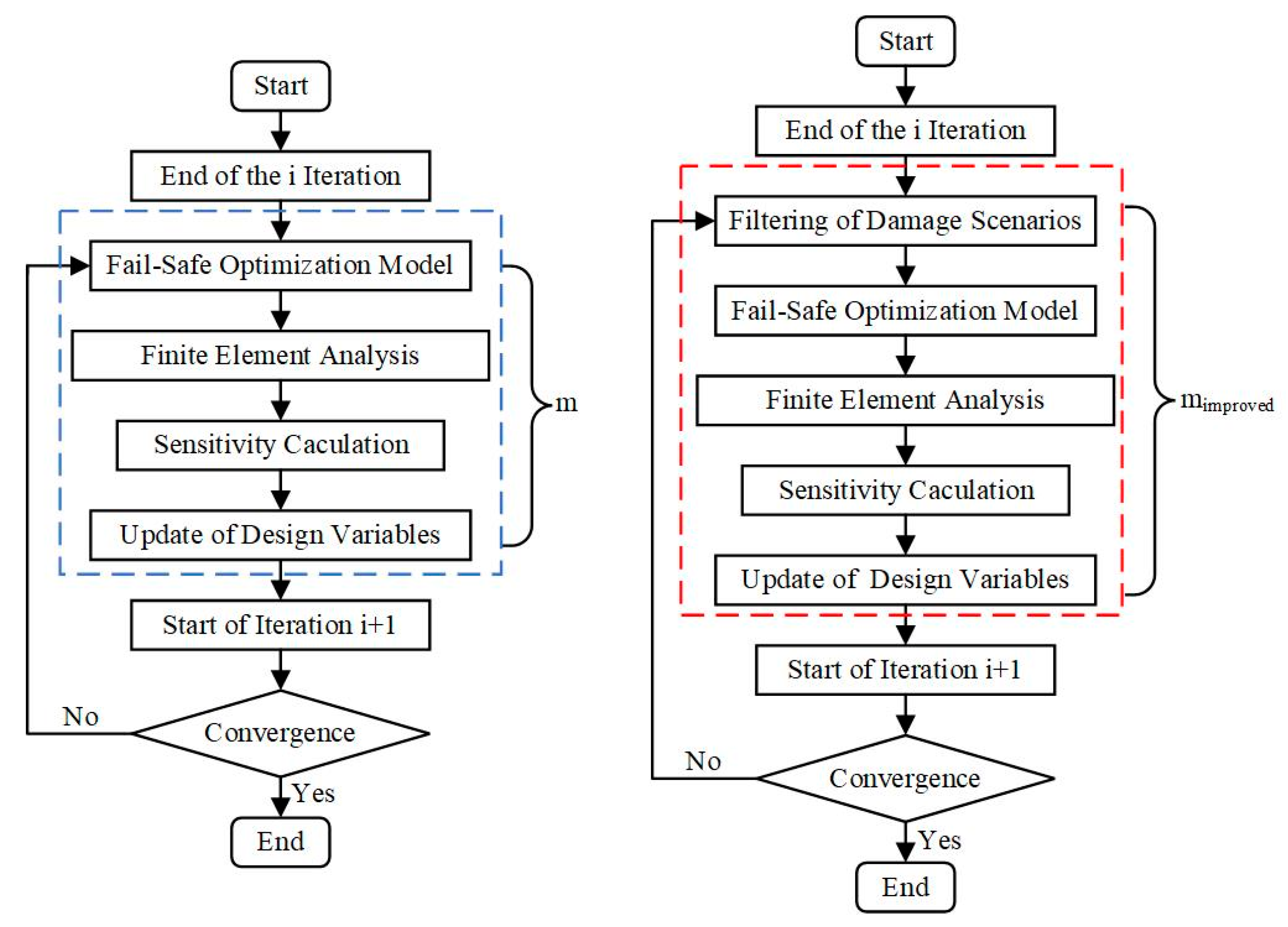Figure 1 illustrates the optimization process for the nth iteration, where ${\mathrm{m}}^{\mathrm{n}}$ represents the number of damage scenarios to be considered, ${\mathrm{m}}_{\mathrm{decrease}}^{\mathrm{n}}$ denotes the reduced number of damage scenarios, and ${\mathrm{m}}_{\mathrm{improved}}^{\mathrm{n}}$ indicates the number of damage scenarios to be considered after adopting the improved algorithm.

For the first scenario, the combined approximation reanalysis method can be employed to enhance the efficiency of obtaining optimization information. The second scenario constitutes a primary focus of this study. Through the extension of the active set method, this approach can be considered as a means of reducing the computational complexity of fail-safe structural optimization by simplifying the number of local damage scenarios.

When addressing issues that are present in standard fail-safe topology optimization, the use of density-based filters is employed to calculate the unit densities in the local damage region. This, in turn, allows for the assessment of the impact of local damage on the structure, eliminating situations where there are either no units or very few units in the local damage region. This ensures that even with a loss in stiffness of certain materials in the design domain, the structure’s overall integrity remains largely unaffected.

In the aforementioned context, there is no longer a need to perform sensitivity calculations for local damage scenarios. It suffices to consider the sensitivity information under the corresponding damage scenarios as the sensitivity information for the structure without local damage. Referring to Figure 2, one can comprehend the distinctions among traditional topology optimization methods, fail-safe topology optimization methods, and the improved fail-safe optimization method employed in this study, especially regarding the number of finite element analyses and sensitivity calculations during the optimization process.

$$A_0={\displaystyle \underset{N_i\in \Omega }{\int }\rho \left({\mathrm{x}}_i\right)}d\mathsf{\Omega }$$

(14)

where ${\mathrm{A}}_0$ is defined as the sum of the unit density in the damaged area by comparing it to the predefined density threshold, ${\mathrm{A}}_{}$, and regions where ${\mathrm{A}}_0\le \mathrm{A}$ are considered to contribute lower than the given threshold and are excluded from further optimization, thus disregarding failure. Conversely, regions where ${\mathrm{A}}_0\ge \mathrm{A}$ are identified as failure areas contribute higher than the threshold, and they are simulated for failure in subsequent optimizations. Adjusting the threshold reasonably helps regulate the number of damage scenarios, thereby enhancing the computational efficiency of the fail-safe optimization method. To enhance readers’ comprehension of this approach, pseudo-MATLAB code will be presented in Algorithm 1.

Algorithm 1. Density Filtering Algorithm

Input: nelx (elements in the horizontal), nely (elements in the vertical) $V\left(\rho \right)$ and $r_{\min }$

Initializing material parameters: $E$ (Young’s modulus), $\upsilon$ (Poisson’s ratio), $\mathrm{A}$ (density threshold);

loop = 0

while (loop <= 250) && (change > 0.01)

loop = loop + 1;

Solve the finite element problem $Ku=f_{}$;

for i = 1: falepatch

Use (14) to compare the sum of patch failure densities ${\mathrm{A}}_0$ with the density threshold $\mathrm{A}$;

Find all failed patches (falepatch) based on density filtering;

Stiffness matrix for assembly failure case ${{\rm K}}^m$;

Solve the finite element problem for the primary failure case $K^m{u}^m=F$;

Use (9) to calculate the sensitivity for each failure;

end

Integration gives total sensitivity information;

Update design variables using the F-S-OC method;

end

Output: physical density $\rho$

3. Numerical Benchmarks

In this section, the performance of the proposed fail-safe improvement method will be demonstrated through a comparison with traditional fail-safe topology optimization. Henceforth, the conventional fail-safe topology optimization will be referred to as the general fail-safe optimization method. It is worth noting that while a non-overlapping distribution of patches is sufficient to achieve viable solutions, its drawbacks are also evident. Therefore, to attain a standardized fail-safe optimization design, Jansen’s fail-safe framework is employed in the majority of cases. Throughout all subsequent chapters, unless otherwise specified, the material properties for a homogeneous solid are as follows: Young’s modulus of E = 1 and Poisson’s ratio of ν = 0.3. In the examples below, following Zhou’s recommendation and considering the practicalities of fail-safe topology optimization, the maximum iteration count is set to 250 for the cantilever beam case and 100 for the L-shaped beam case, as defined in the relevant examples.

3.1. Cantilever Beam

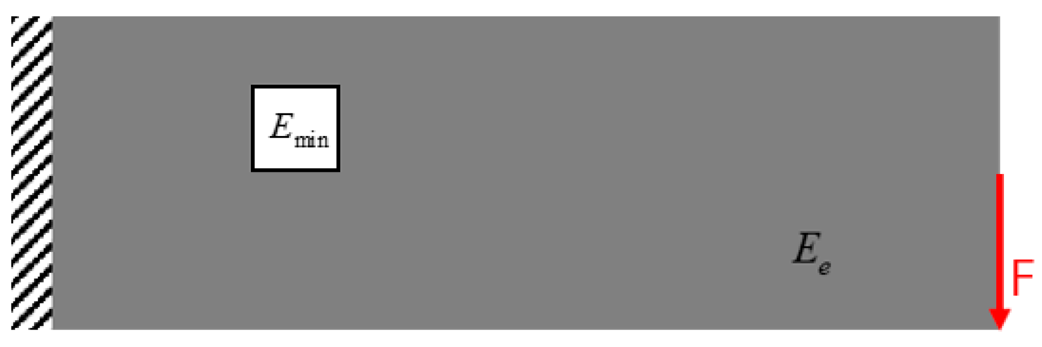
Taking the cantilever beam, which is frequently discussed in many reference studies, as an example (as shown in Figure 3), the design domain of the cantilever beam is discretized into 120 × 40 elements, forming a total of 4800 elements. The entire design domain consists of 4800 elements. A vertical load (F = 1) is applied at the bottom right corner of the cantilever beam, with a fixed constraint applied to the left edge of the cantilever beam. The volume fraction of the solid material to be preserved is limited to 0.4, representing the deformation energy of the structure under local damage, as well as the proportion of the second local failure scenario in all failure scenarios. Subsequently, we can establish a density iteration.

Firstly, the cantilever beam is optimized to achieve a patch size of 5 × 5. Additionally, local damage near the loading position, indicated by the red arrow, is not considered during the optimization process. The loading conditions remain unchanged, mitigating the impact of stress concentration at the loading point.

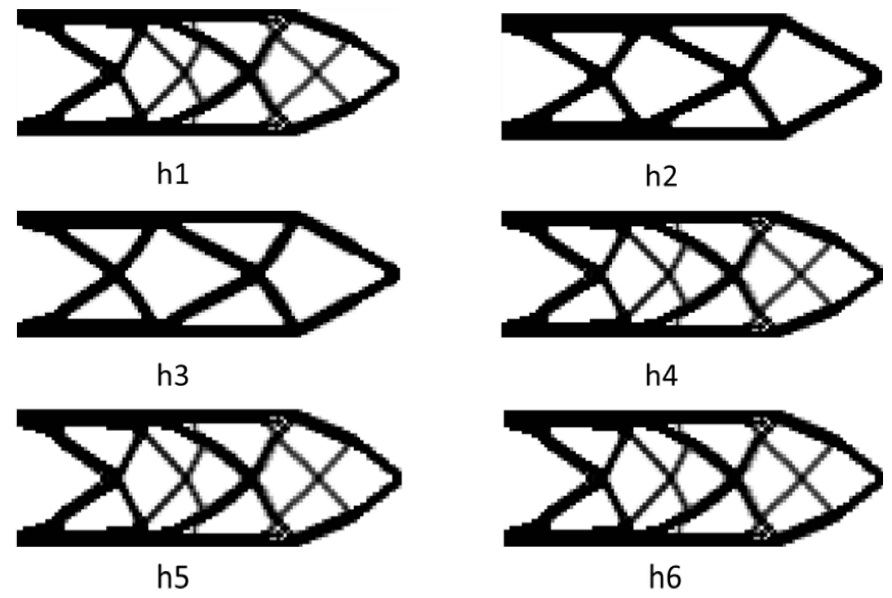
Figure 4 presents the optimized cantilever structure obtained through the fail-safe optimization algorithm for the damage model (L = 5). This includes designs from both traditional fail-safe optimization and the improved algorithm. The nominal design represents the optimization result from the traditional algorithm, while the others denote fail-safe optimization designs from the improved algorithm. In the designs obtained through the improved algorithm, adjusting the threshold of the density filter to 0.01, 0.1, 1, 2, and 4, respectively, produces corresponding fail-safe optimization designs. Comparing the designs obtained through the improved algorithm with those from the standard fail-safe optimization algorithm reveals that the improved fail-safe optimization algorithm not only achieves the desired fail-safe optimization designs, but also significantly reduces the computational effort required for optimization. As shown in Figure 4 and Figure 5, the larger the threshold of the filter, the smaller the computational effort needed for the optimization process.

Figure 6a illustrates the cantilever structure obtained through the nominal fail-safe optimization algorithm when adjusting the size of the local damage model to L = 14. As the area of the local damage region increases, the threshold of the damage scenario filter also needs to increase, set at 10, 21, 32, 43, and 54, respectively. From Figure 6 and Figure 7, it is evident that the enhanced fault-tolerant optimization algorithm can achieve the desired structural design and reduce the computational effort required for optimization. However, as the filter threshold increases, the difference between the design obtained through the improved algorithm and the standard design becomes more significant. Clearly, the optimization process deviates from the correct direction, which is not the expected outcome. The judicious and efficient selection of the filter threshold value warrants further research, which is not detailed here.

Table 1. Reduction rate in the average iteration time during the optimization process of the cantilever beam.

L = 5	A	0.01	0.1	1	2	4
	Rate	13.7%	13.9%	22.2%	26.7%	35.8%
L = 14	A	10	21	32	43	54
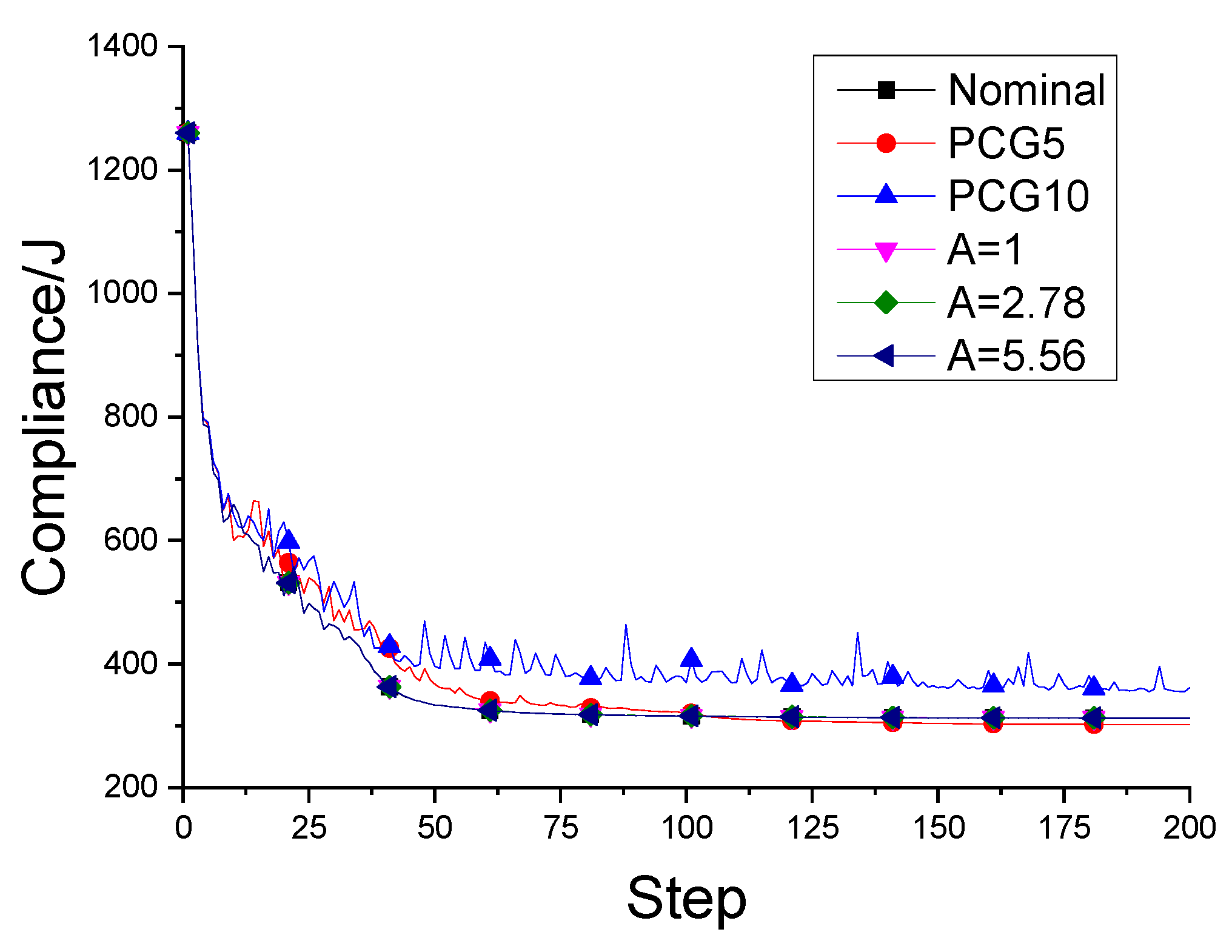
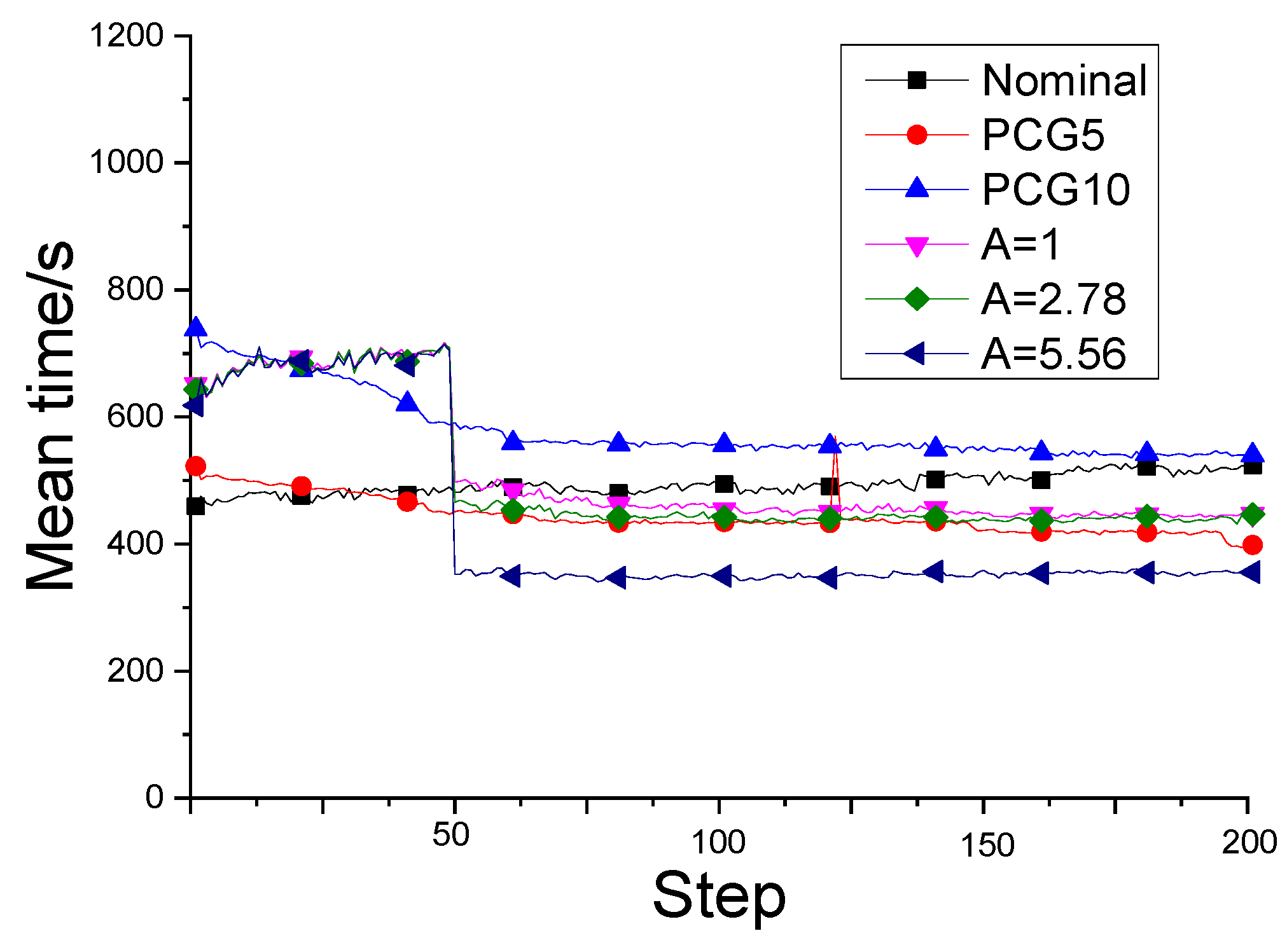
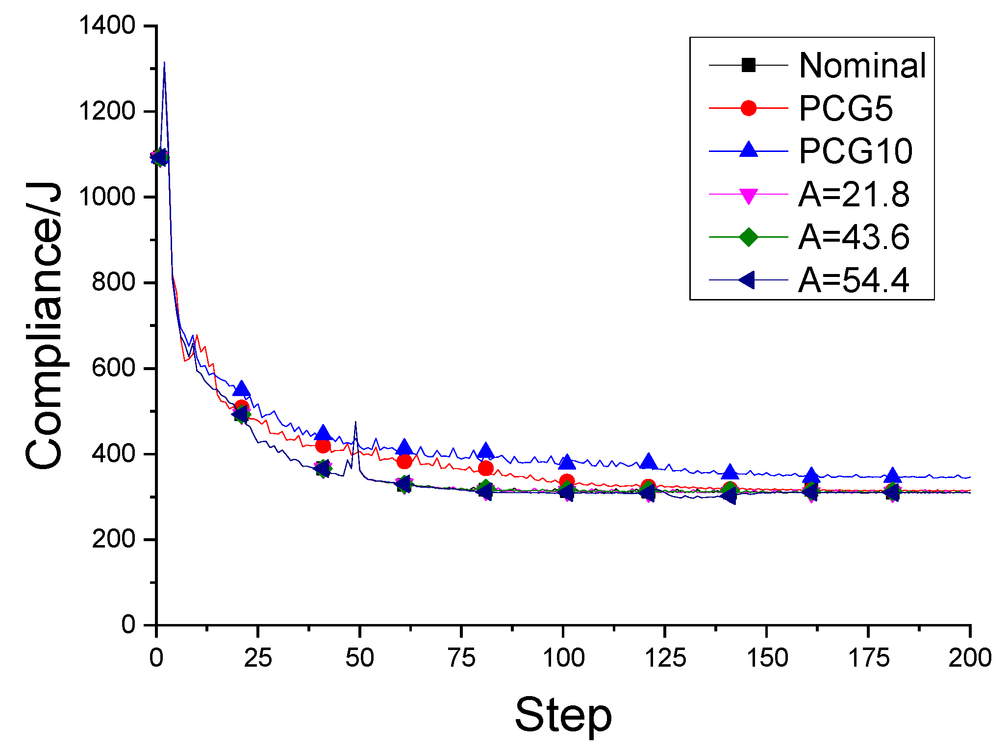
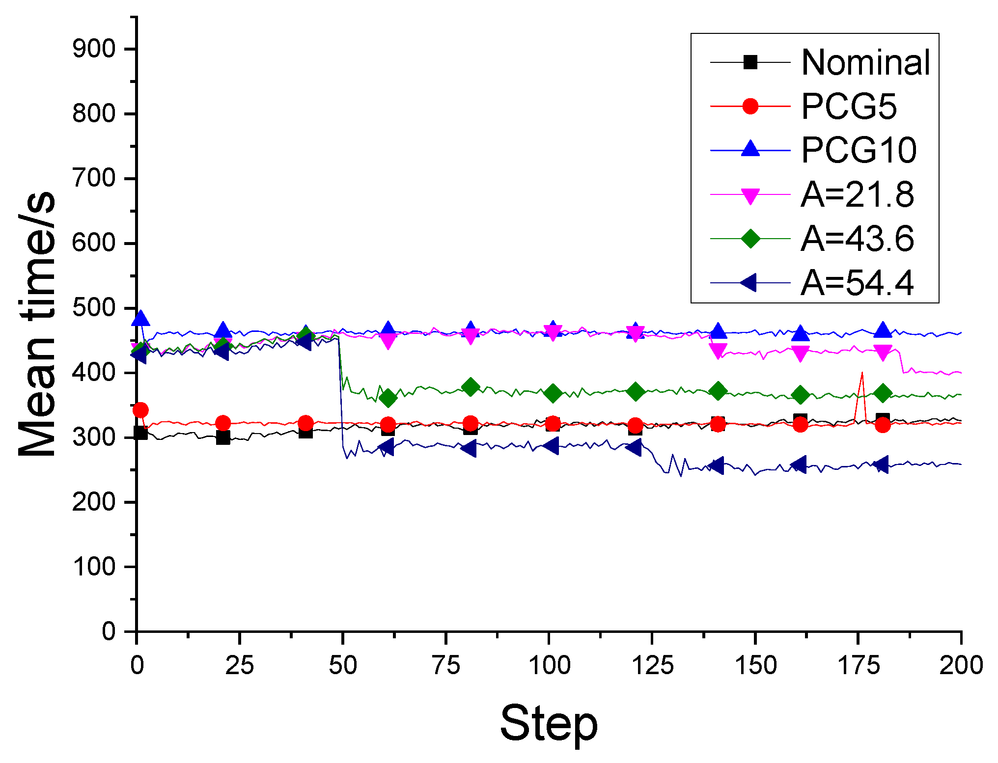
	Rate	0	0	1.6%	16.1%	35.6%

displays the adjustment of the filter threshold to filter local damage scenarios, leading to a reduction in the rate of iteration steps during the optimization process of the improved fail-safe optimization method. It is evident that the average iteration time during the fail-safe optimization process continuously decreases with the increase in the threshold. Clearly, by assessing the effectiveness of the local damage scenarios, the topological optimization calculations for fail-safe structures can be significantly reduced. Furthermore, this study seamlessly integrates the preconditioned conjugate gradient method with the fail-safe topology optimization algorithm to enhance the computational efficiency of the fail-safe topology optimization algorithm. For detailed information on the optimization results and computational efficiency of traditional fail-safe optimization algorithms, PCG fail-safe optimization algorithms, and density filter-based fail-safe optimization algorithms, please refer to Appendix A.

3.2. L-Bracket

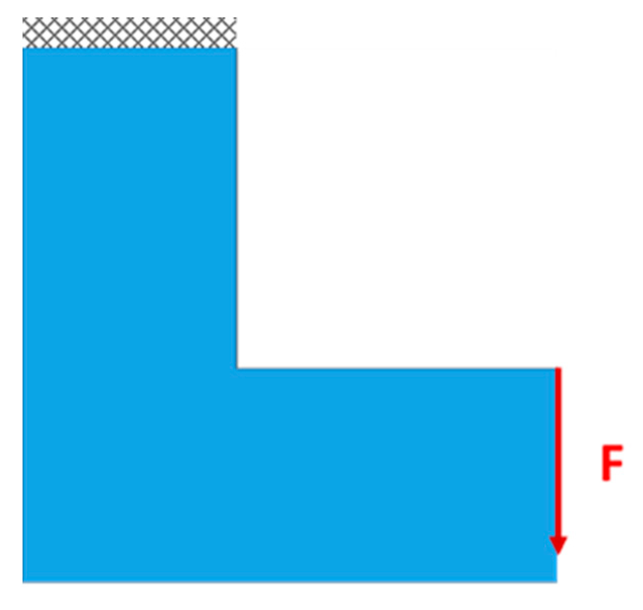
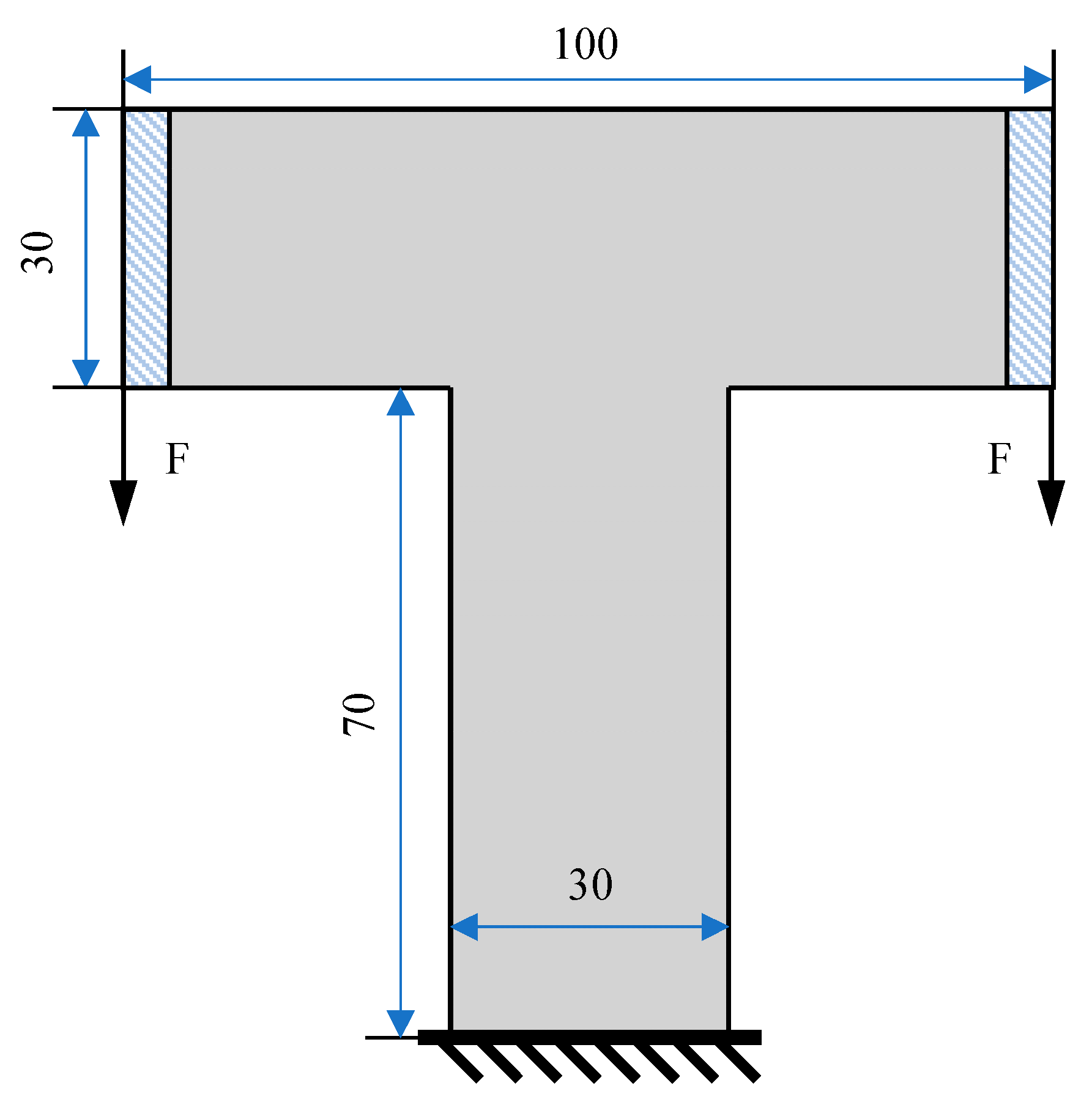
The well-known L-shaped beam, as illustrated in Figure 8, is discretized using four-node finite elements with a size of 1 × 1 mm², resulting in a total of 10,000 elements. In the final topology, only 35% of the material is available. The top of the L-shaped bracket is fixed, and an external load (F = 1) is applied at the bottom right corner, as shown at the top of Figure 8. The gray area in the figure represents the prescribed non-active region. The width of the non-active region is equal to the side length of the local damage model.

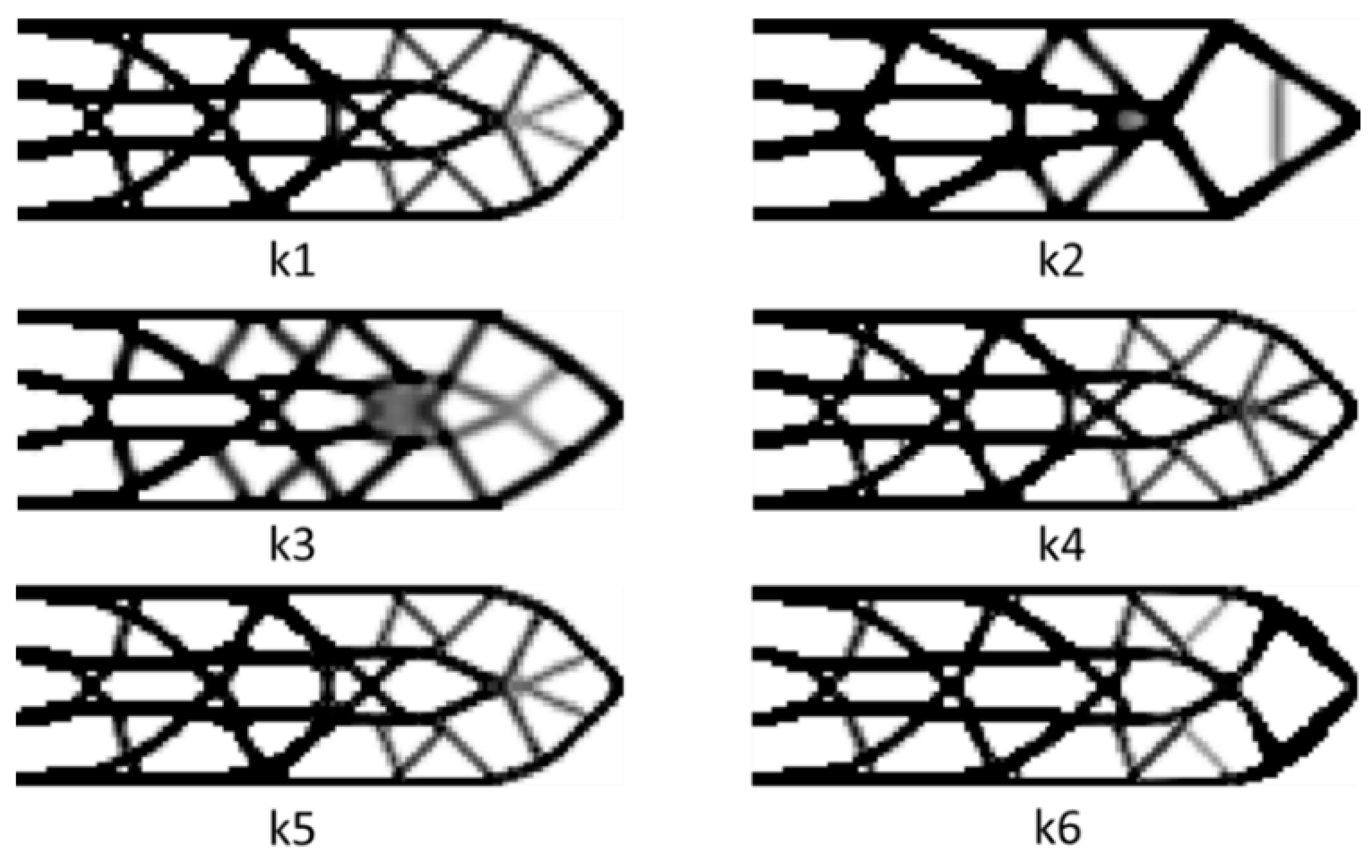
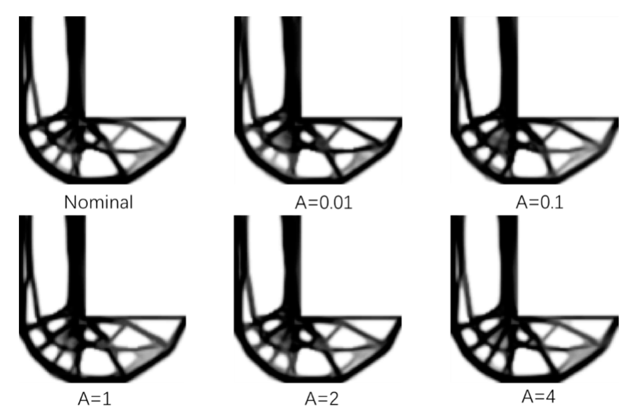
The dimensions of the local damage model are L = 4, used to optimize the L-shaped bracket. Figure 9 displays the L-shaped bracket structure obtained through the standard fail-safe optimization method, followed by the improved structural design using the fail-safe topology optimization algorithm. The density filter ‘A’ threshold is adjusted to 0.01, 0.1, 1, 2, and 4, respectively. From the final results, it is challenging to discern significant differences between them. When the side length of the damage model is L = 4, the optimization results from both the traditional fail-safe optimization method and the improved fail-safe optimization algorithm with different thresholds are nearly identical.

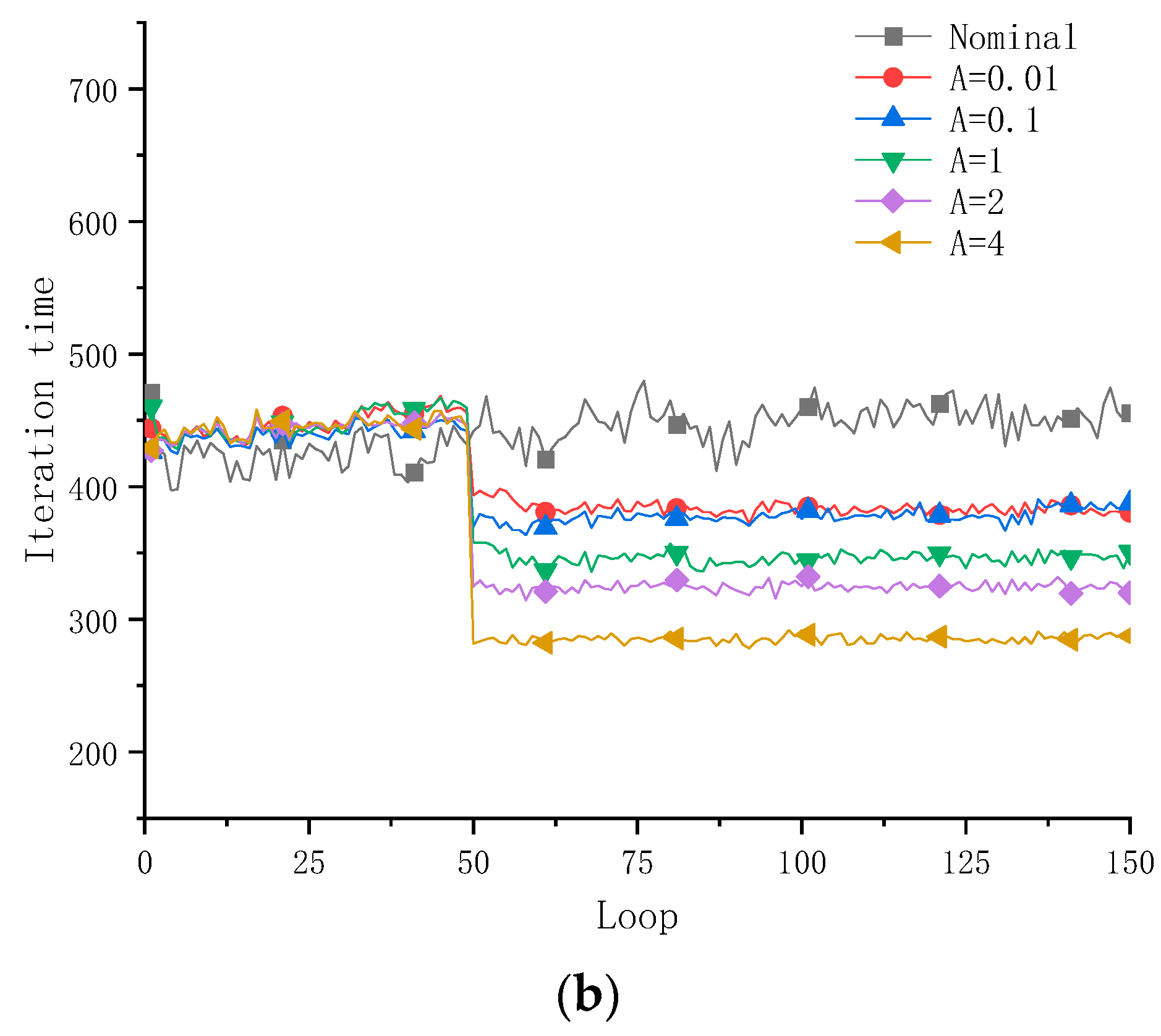
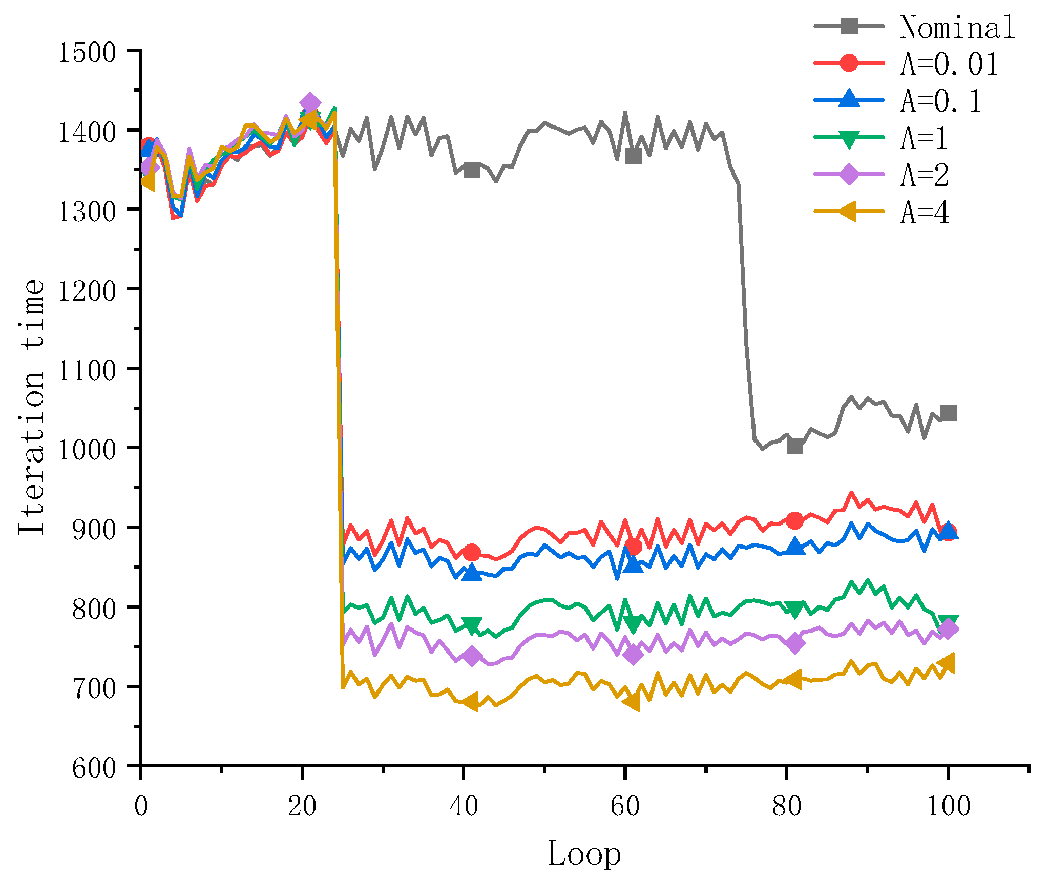
Figure 10 illustrates the iteration time curves for the density-filtered failure-safe optimization method under the condition of a local damage model with L = 3. The filter thresholds are set to 0.01, 0.1, 1, 2 and 4, and a comparison is made with the standard failure-safe optimization method. In Figure 11, the horizontal axis represents the filter threshold, while the vertical axis depicts the reduction in the average iteration steps during the optimization process and the fail-safe topology optimization, respectively (for varying thresholds). 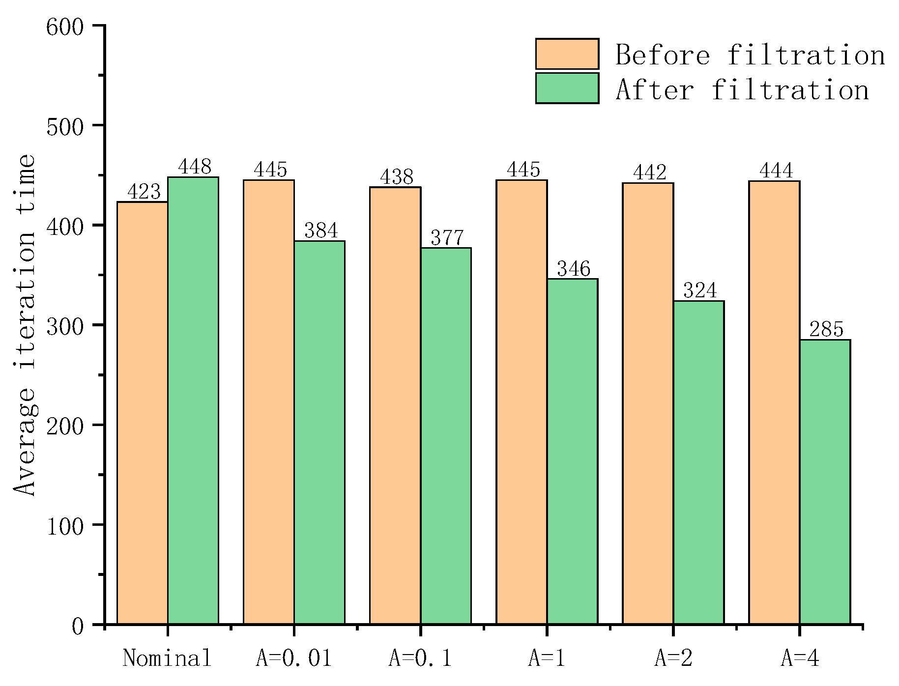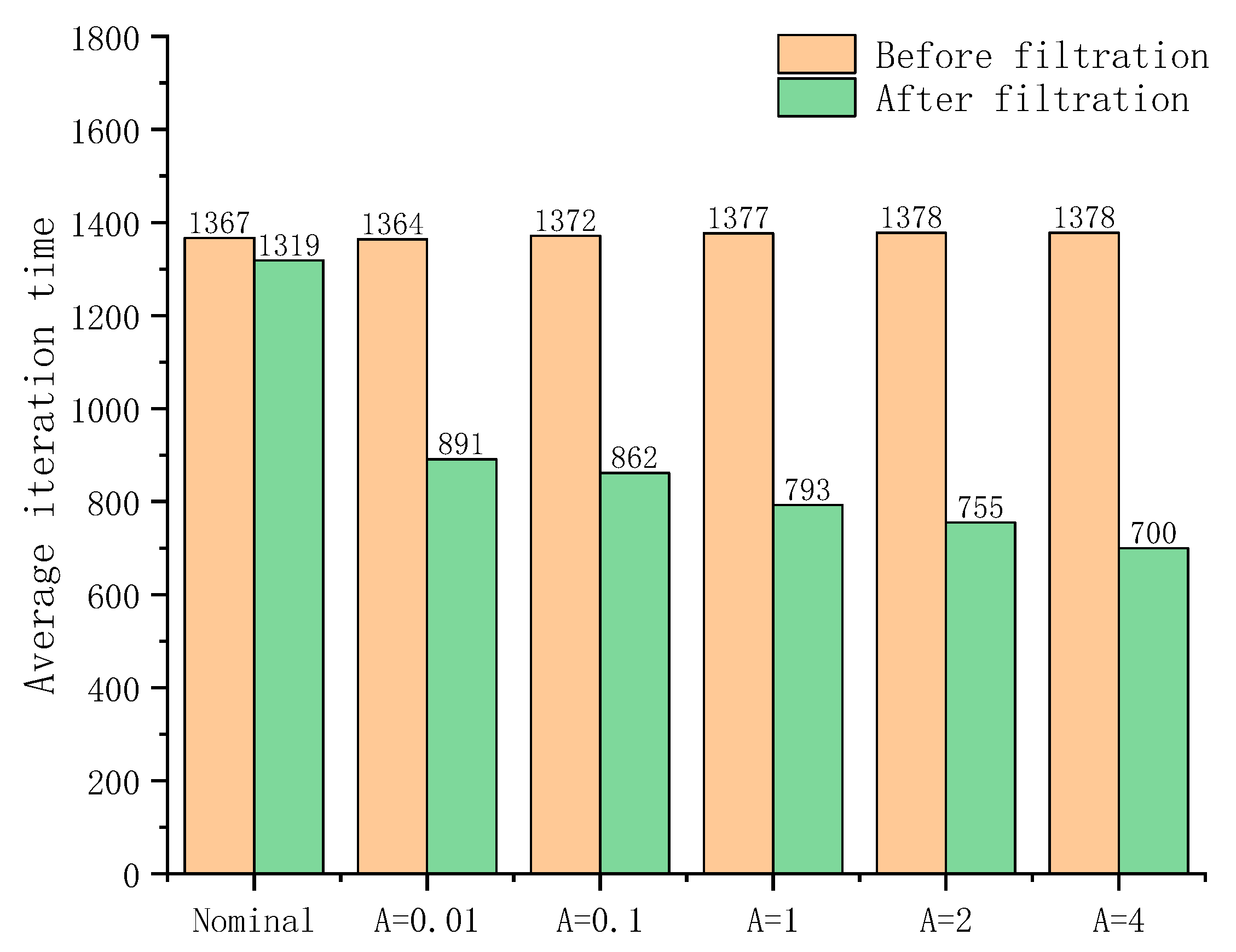Figure 12 illustrates the average iteration time before and after the improvement of the fail-safe structural optimization method.

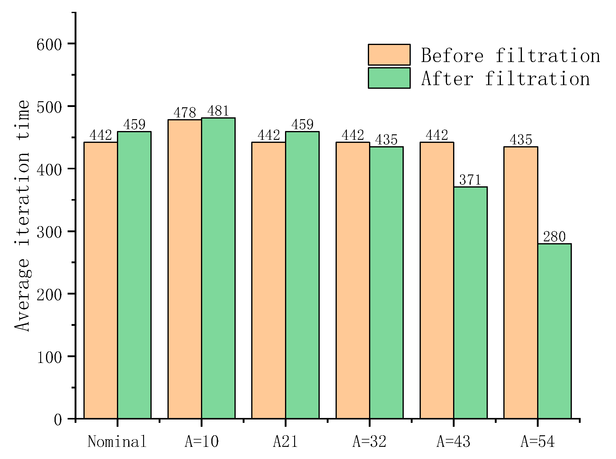
Figure 13 depicts the fail-safe optimization designs for the L-shaped bracket obtained using the fail-safe optimization method with a local damage model size of L = 6 and filter thresholds set to 0.01, 0.1, 1, 2, and 4. After analyzing the optimization results of both the standard fail-safe optimization method and the improved fail-safe optimization method, it can be observed from Figure 13 and Figure 14 that the larger the threshold of the density filter, the greater the differences between the final optimization results of the respective algorithms.

Additionally, with the increase in the filter threshold, the time required for each iteration during the optimization process gradually decreases. However, when L = 6, although the entire optimization solution can converge to the optimal structure, stability issues may arise during the optimization process. This is because the size of the local damage model directly affects the variation in sensitivity information during the optimization process. As the scale of the local damage model increases, stability and convergence issues in the optimization process become more pronounced.

By observing

Table 2. Reduction rate in the average iteration time during the optimization process of the L-shaped beam.

L = 4	A	0.01	0.1	1	2	4
	Rate	34.7%	37.2%	42.4%	45.2%	49.2%
L = 6	A	0.01	0.1	1	2	4
	Rate	26.1%	27.0%	29.5%	31.3%	33.8%

, it can be noted that by adjusting the threshold of the filter, the computational effort required for fault-tolerant structural topology optimization can be effectively reduced. When L = 4, the average iteration steps for fail-safe structural optimization can be reduced by over 35%, and when L = 6, the average iteration time can also be reduced by 25%. This method is evidently feasible for the entire fail-safe optimization process. However, it is worth noting that there is an upper limit to the threshold. Excessively high thresholds may cause the optimization to deviate from the correct direction, resulting in the presence of ineliminable intermediate density elements. This becomes particularly evident when the local damage area is large.

3.3. T-Shaped Beam

To test whether this method could verify more complex scenarios, the T-shaped beam mentioned by Wang et al. [42] is considered in this case. As shown in Figure 15, the design space of the T-shaped beam is discretized, encompassing a total of 5100 elements. The bottom of the T-shaped beam is supported, and vertical loads (F = 1) are applied at the lower corners of the left and right boundaries. The volume fraction of the solid material to be preserved is constrained to 0.4. Each failed patch covers 10 × 10 elements. The blue regions in the figure represent inactive areas, with each inactive area covering 5 × 30 elements. The density threshold is set to A = 10.

Firstly, the T-shaped beam is optimized so that the patch size is 5 × 5. In addition, the local damage near the loading position, that is, at the red arrow, is not considered in the optimization process. The loading conditions are kept unchanged, and the influence of stress concentration at the loading point is avoided.

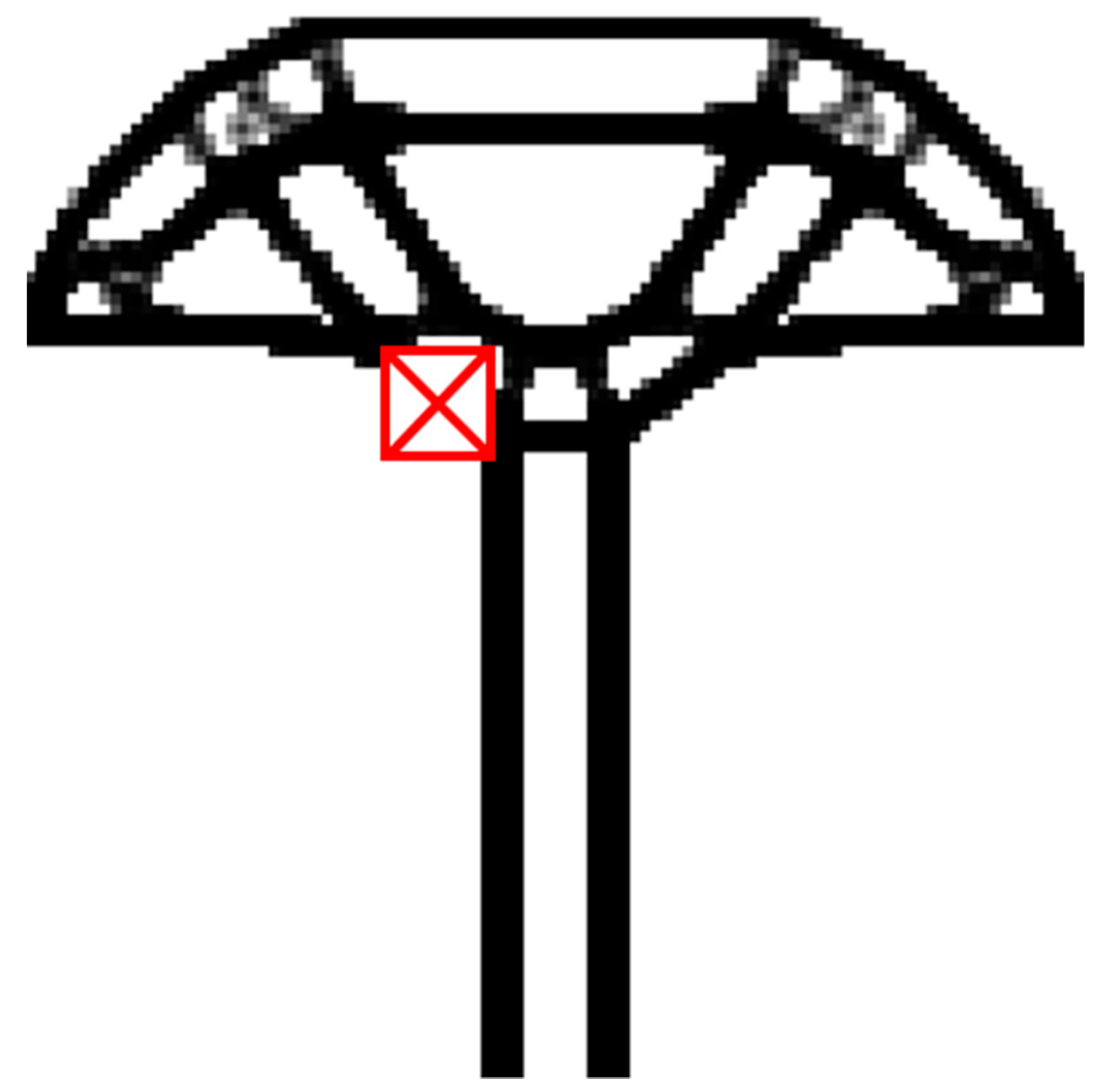
As shown in Figure 16, the aforementioned T-shaped beam still obtains a clear configuration under the corresponding conditions. Simultaneously, under these conditions, the optimally worsened damaged area of the structure is represented by a red square, corresponding to a strain energy of 184.02. In order to observe and locate weak areas within the structure (stress concentration), a stress analysis of the aforementioned structure is conducted.

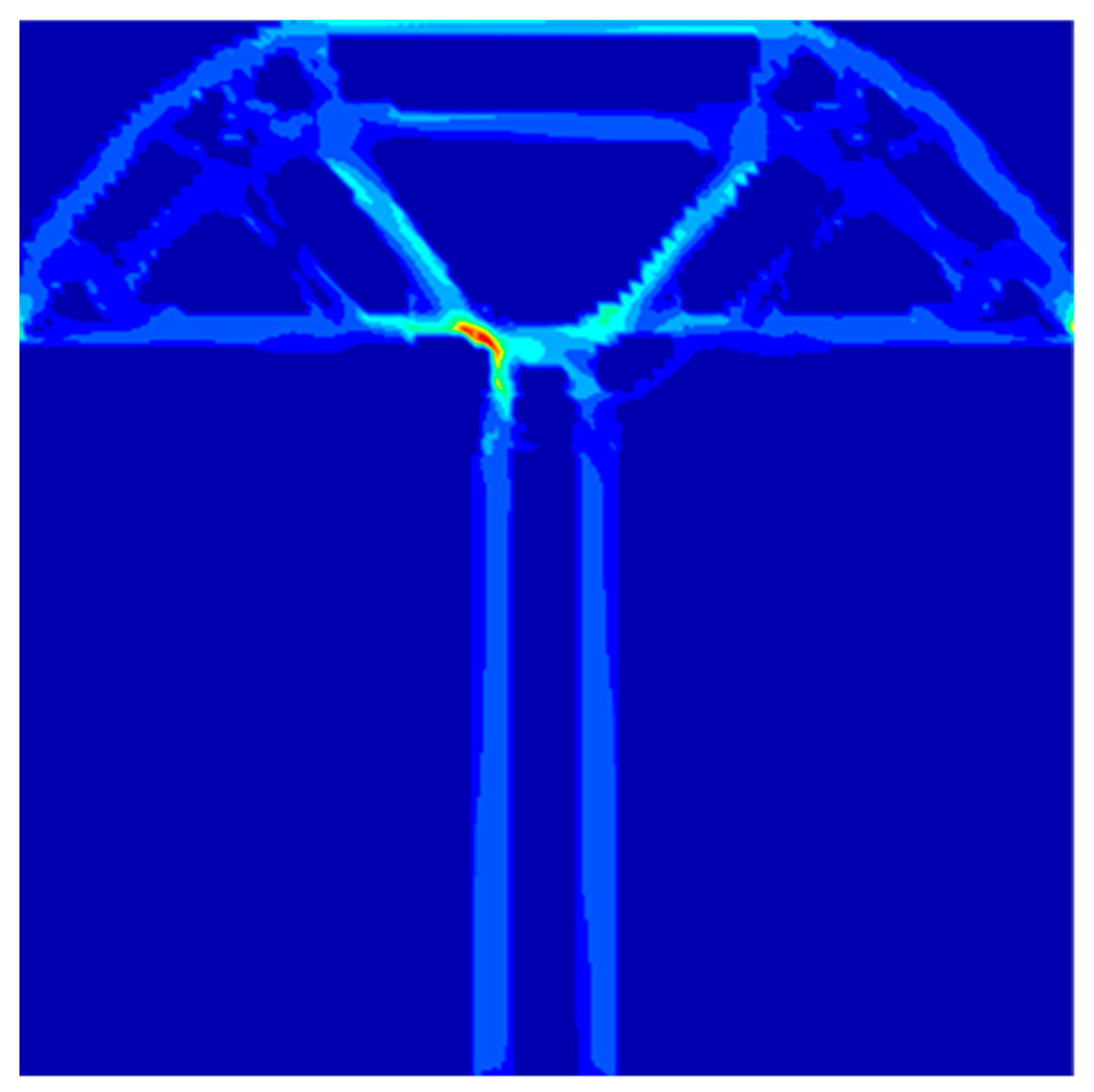
As shown in Figure 17, the maximum stress is ${\sigma }_{\max } = 1.564$. By comparing the two optimized result diagrams, it is evident that the most severe damaged areas are identical. Filtering through density thresholds not only ensures reduced sensitivity to failure but also enhances the computational efficiency. Consequently, fail-safe topology optimization filtered by density thresholds can efficiently achieve a highly robust fail-safe design.

4. Discussion

To enhance the computational efficiency of the fail-safe topology optimization method, a density-based filter has been introduced to determine whether additional finite element analyses and sensitivity calculations are necessary when traversing local damage scenarios. A comparative analysis of the optimization results reveals that this approach can significantly reduce computational efforts, especially in scenarios involving extensive damage. The locally simplified damage scenario method based on density filtering ensures optimization precision, thereby improving the computational efficiency of the fail-safe structural topology optimization algorithm. Additionally, considering some prior knowledge of the optimization model, such as the symmetry of the structure or load during the optimization process, further enhances the computational efficiency of the fail-safe topology optimization algorithm.

However, this study is limited to the research on structural fail-safe topology optimization algorithms in the elastic phase, without considering fail-safe optimization designs after structural plastic deformation. Determining the regularization parameter poses a challenging question. In fail-safe topology design, unreasonable regularization parameters often lead to more unnecessary details or the appearance of numerous intermediate density elements in the optimization results. Therefore, for the efficient and rational selection of regularization parameters in plastic phase fail-safe topology optimization algorithms, further in-depth research and exploration are needed.