Abstract
With the rapid development of artificial intelligence technology, the physics-informed neural network (PINN) has gradually emerged as an effective and potential method for solving N-S equations. The treatment of constraints is vital to the PINN prediction accuracy. Compared to soft constraints, hard constraints are advantageous for the avoidance of difficulties in guaranteeing definite conditions and determining penalty coefficients. However, the principles on the formulation of hard constraints of PINN currently remain to be formed, which hinders the application of PINN in engineering fields. In this study, hard-constraint-based PINN models are constructed for Couette flow, plate shear flow and stenotic/aneurysmal flow with curved geometries. Particular efforts have been devoted to assessing the impact of the model parameters of hard constraints, i.e., degree and scaling factor, on the prediction accuracy of PINN at different Reynolds numbers. The results show that the degree is the most important factor that influences the prediction accuracy, followed by the scaling factor. As for the N-S equations, the degree of hard constraints should be at least two, while the scaling factor is recommended to be maintained around 1.0. The outcomes of the present work are of reference value for the development of PINN methods in fluid mechanics.
1. Introduction
Over the past five decades, there have been substantial advances in developing computational fluid dynamics (CFD) techniques to numerically solve Navier–Stokes (N-S) equations for fluid mechanics in real-world applications [1,2]. In conventional CFD methods, e.g., the finite-difference (FD) and finite-volume (FV) methods, sophisticated computational grids are required for domain discretization, especially when complex geometries are involved. The generation of high-quality grids makes CFD computations cumbersome and is always demanding for CFD engineers. On the other hand, due to the lack of high-performance generic algorithm libraries, developing flow solvers based on conventional CFD methods is always challenging and time-consuming for CFD developers. Machine learning, as a main branch of artificial intelligence (AI) and computer science, can be used to solve partial differential equations (PDEs) including N-S equations with avoidance of the above problems of CFD methods [3,4], which creates new horizons and possibly even transformations for the current lines of fluid mechanics research.
Depending on the manners by which the ML approaches are integrated with CFD solvers, ML approaches for fluid mechanics can be roughly categorized into three classes, i.e., data-fit models, projection-based models and physics-informed models. A data-fit model is usually based on the artificial neural network (ANN) [5,6], radial basis function (RBF) [7] and support vector regression (SVR) [8,9], and it treats a CFD solver as a black box and is essentially a fast, inexpensive but approximate model that extracts mechanisms underlying the complex system from available data in a supervised manner. Data-fit models have been widely used as a substitute for expensive CFD simulations in design optimization or uncertainty quantification of fluid systems [10]. However, constructing such types of models requires additional overhead of data simulation, which could become expensive and even unaffordable for high-dimensional problems. As for projection-based models, an orthogonal linear transformation is first defined from physical coordinates into a modal basis in an unsupervised manner by means of principle orthogonal decomposition (POD) or other methods, and then the PDE operator is projected onto the subspace spanned by the reduced modal basis [11,12]. Although the degree of freedom of solution can be significantly reduced, projected-based models need modifications of the original CFD codes, and the issues of stability and robustness are still not well addressed. Different from the above two types of models, physics-informed models embed a priori physics into the learning architecture, which not only remains code-nonintrusive but also reduces the dependency on data availability [13]. Owing to the rapid advances in deep learning, the current mainstream of physic-informed models is the physics-informed neural network (PINN) [14,15], whereby the PDEs are directly incorporated in the loss function of the neural network by penalizing deviations from the target values.
So far, PINN models have been successfully applied in solving incompressible and compressible flows [16], and there are basically two application scenarios, i.e., inverse and forward problems. In inverse problems, parameters of the equation (including definite solution conditions) and flow field are partly known while the remaining ones need to be solved, which is thus considered to be a semi-supervised problem. For example, Raissi et al. [17] proposed a “hidden fluid mechanics” framework based on PINN and successfully identified unknown equation parameters and inversed the velocity and pressure of the flow around a cylinder with the concentration field provided. Mao et al. [17] solved the density, velocity and pressure of the Sod and Lax problems by PINN with the density gradient and pressure of some samples given in advance. As can be seen, the solution accuracy of the inverse problem is still dependent on prior information. On the contrary, the forward problem could be an unsupervised one where only governing equations and definite solution conditions are known and all the flow quantities are to be solved. For example, by using the PINN model, Sun et al. [18] accurately predicted the velocity field of Couette flow, stenosis flow and aneurysm flow. Jin et al. [19] adopted a similar method to predict the turbulent channel flow without any physical information given in advance.
Although solving the forward problem by PINN does not necessarily rely on any prior information, constraint enforcement should be paid particular attention to guarantee the model prediction accuracy at the specific definite condition. This is because PINN modeling is essentially an optimization problem, and the accuracy of the model is closely associated with the way the constraints are enforced. The constraint enforcement method of PINN can be generally divided into two categories, i.e., the “soft” constraint method and the “hard” constraint method.
In the soft constraint method, the original optimization problem is transformed into an unconstrained one by adding penalty terms of initial conditions (ICs) and boundary conditions (BCs). Jagtap et al. [20] constructed PINNs with soft constraints based on an adaptive activation function to solve PDEs including the nonlinear Klein–Gordon equation, the nonlinear Burgers equation and the Helmholtz equation. Wang et al. [21] presented a learning rate annealing algorithm to solve the numerical stiffness problem in solving PDEs with PINN. Jagtap and Karniadakis [22] integrated the space–time domain decomposition method into the soft-constraint-based PINN framework to parallelize the computations. Despite the inspiring progress in solving PDEs, the soft constraint method for PINN still has two major disadvantages, as Sun et al. [19] pointed out. First, it can hardly guarantee that the network output fully conforms to ICs and BCs, thus giving rise to the loss of prediction accuracy of PINN; second, the involved penalty coefficients are often difficult to determine, either relying on experience or requiring trial and error, which is also detrimental to the modeling efficiency of PINN.
The hard constraint method can circumvent the above problems by introducing a particular solution and a smooth function that enables the PINN prediction results to satisfy ICs and BCs in a mandatory manner. The particular solution can be solely determined according to ICs and BCs, while the smooth function connects the boundary to the internal domain, which is crucial to the PINN prediction accuracy. In the work by Sun et al. [19], the PINN prediction results with hard constraint were in good agreement with FV-based CFD results, while those with soft constraint deviated significantly from FV-based CFD results. However, no principles were given in their work for the formulation of smooth functions in the hard constraints. To the best knowledge of the authors, no further study has been conducted on how to formulate hard constraints for PINN, which to some extent hinders the application of PINN in realistic engineering fields.
The purpose of this study is twofold. The first is to investigate the effect of parameters in the smooth function on the PINN prediction accuracy, where several flows including Couette flow, plate shear flow and stenotic/aneurysmal flow at different Reynolds numbers are examined. The second is to provide guidelines for the formulation of hard constraints for PINN modeling. The rest of this paper is organized as follows. Section 2 describes the basis of the PINN model and constraint methods. In Section 3, some numerical tests are carried out, and formulation principles of hard constraints are summarized from the corresponding results. PINN solutions of Couette flow, plate shear flow and stenotic/aneurysmal flow under different values of degree and scaling factor are shown in Section 3. Conclusions are finally drawn in Section 4.
2. Methodology
2.1. PINN Model
The N-S equations to be solved by PINN can be mathematically expressed as:
where both velocity and pressure are functions of space coordinate and time coordinate ; and denote the flow density and viscosity, respectively. For all the flows investigated in this study, is set to be 1; and represent the boundary conditions (BC) and initial conditions (IC), respectively; and are known continuous functions.
Similar to most ANNs, the PINN is a multi-layer perceptron that builds an explicit relationship between input and output. As for the above N-S equations with the predicted velocity and pressure of an n-layer PINN denoted as and , respectively, we have:
where represents the operation function corresponding to the i-th layer and is usually expressed as:
where is the output of the i-th hidden layer, is the activation function and and represent the related weights and thresholds, respectively.
The primary idea of the solving method for N-S equations based on the PINN is to find a set of appropriate model parameters to minimize the residual of the equation with the related BC and IC enforced with the constraints, i.e.,
where is the so-called “physical-based loss function”. It reflects the degree to which the knowledge learned by the neural network fits with the given differential equations and definite solution conditions.
2.2. Constraint Enforcement Method
In order to solve the optimization problem presented in Equations (7)–(9), proper constraints should be enforced to guarantee the ICs and BCs in Equation (9). As previously mentioned, there are two ways to enforce the constraints in PINN modeling, i.e., the soft constraint method and the hard constraint method.
In the soft constraint method, the original constrained optimization problem is transformed into an unconstrained one by adding penalty terms of ICs and BCs [23], i.e.,
where and represent the loss of network output in BC and IC, respectively, while and are the related penalty coefficients and are usually determined by experience or trial and error.
To avoid difficulties for the soft constraint method in guaranteeing definite conditions and determining penalty coefficients, the hard constraint method is employed in the present work. In this method, a particular solution and a smooth function are introduced to modify the network output, enabling the ICs and BCs to be mandatorily satisfied, i.e.,
where and denote the PINN-predicted results of velocity and pressure; and are referred to as the particular solution that solely satisfies IC and BC; is defined as the smooth function from internal points to the boundary, which is equal to 0 on and while being non-zero continuous values in other regions. Accordingly, the final result will not fail to satisfy the boundary condition due to the change in or . Hence, the original optimization problem described in Equations (7)–(9) can be transformed into the following unconstrained one, i.e.,
Therefore, the main uncertainty of the above “hard” method lies in the mathematical expression of the function , which is considered to play an important role in the prediction accuracy of PINN. Particular attention is thus paid to exploring a general formulation principle of in this study, as presented in the next section. In Equation (18), the derivatives of the outputs with respect to the network inputs are calculated by the automatic differentiation (AD) [24], which is based on the chain rule. The AD tool has been widely used to calculate partial derivative terms of physical quantities in studies of PINN methods [17,18,19,20,21,22,23].
3. Numerical Tests
Since the flows studied in this paper are steady ones, the initial conditions are not involved in the constraint enforcement of PINN, and the time-derivative term in Equation (18) is omitted. In order to adopt the PINN model to solve the above N-S equations, three back propagation neural networks are constructed to build an explicit relationship between the input and output. For each neural network, the inputs are the two-dimensional space coordinates while the flow variables to be solved such as axial velocity , radial velocity or pressure serve as the output. Each network has two hidden layers while each layer is equipped with 20 neurons. In addition to the output layer, the Swish function [25] is selected as the activation function of the neural network, i.e.,
To train the constructed NNs, the Adam algorithm is used as the network optimizer [26] with the learning rate set to 1.0 × 10⁻³. Full-batch learning is adopted, for which the batch size is selected as the number of coordinate points in each case. The Kaiming-normalization initialization method [27] is adopted to initialize and within the optimization process. In order to ensure the accuracy of the results, a total of 50,000 epochs are performed for each case, and the iterations are speeded up with the Compute Unified Device Architecture (CUDA) library [28] on a graphics processing unit (GPU). The machine learning platform PyTorch was chosen to build the framework of the above model [29].
3.1. Couette Flow
Couette flow describes the laminar flow in a two-dimensional infinite plate with non-slip boundary conditions. As shown in Figure 1, the length of the plate is set to 1, the distance between plates is set to 0.1 and the static pressure is set to 0.1 and 0.0 at the inlet and outlet, respectively. The corresponding boundary conditions can be written as:
where and represent the streamwise and vertical components of the local coordinates, respectively. The analytic solutions of the flow can be expressed as:
where is the pressure difference between the inlet and outlet. In the following test, the viscosity is varied to control the Reynolds number of the flow. The Reynolds number is defined with , and the fluid velocity at the center line, .
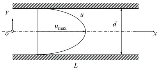
Figure 1.
Schematic of Couette flow. Here, is the plate length, is the plate distance, is the local streamwise velocity and is the velocity at the center line.
To solve the above Couette flow using the PINN model, hard constraints are formulated for the specified boundary conditions, which can be written as:
where and represent the streamwise coordinates of the inlet and outlet of the flow field, respectively; and are the particular solutions of the velocity components and are set to a constant of 0.0 to satisfy the non-slip boundary condition, while is the particular solution of and automatically satisfies the specified inlet and outlet pressure. For the function of , and are the parameters to be determined, where denotes the degree of the function which determines the continuity property of the hard constraints while the scaling factor adjusts the influence of the network output on the final result . In addition, the function of is referring to that in Sun’s work [19], which is quite deterministic and not discussed. Overall, the key to formulating the hard constraints is the selection of the two parameters, i.e., and , in the functions of velocity.
For each simulation case, 25,000 epochs are performed in the training of the PINN model to guarantee convergence. The loss function histories versus epochs at different degree values are given in Figure 2. It can be seen that the training converged after around 15,000 epochs.
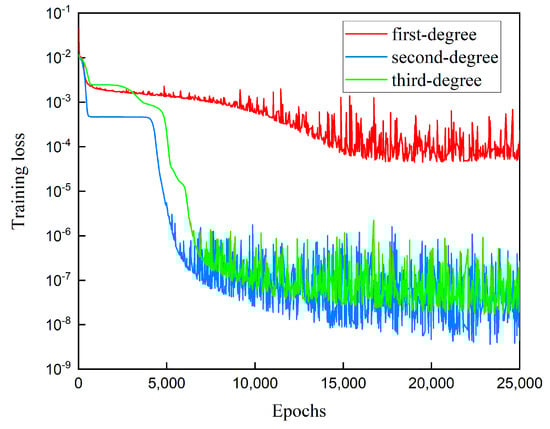
Figure 2.
Training loss histories at different degree values of hard constraint in Couette flow problem.
3.1.1. Effect of Degree
In order to investigate the effect of degree of function D on the PINN-predicted result, three hard constraints with three different degrees (i.e., = 1.0, 2.0, 3.0) and the same scaling factor (i.e., = 1.0) are formulated. The maximum streamwise velocity is used in this flow problem to quantitatively measure the prediction accuracy of PINN, and the comparison between the PINN-predicted results and analytic solutions at different Reynolds numbers is listed in Table 1. As can be seen, the relative errors of the maximum axial velocity between the PINN-predicted results with first-degree hard constraints and analytic solutions are remarkable. However, as the constraint degree increases to 2.0, the relative errors are significantly reduced below 0.1% at most of the examined Reynolds numbers between 139 and 1250 and slightly increased when the Reynolds number increases to 2000. As for the cases with the third-degree hard constraints, the relative errors are larger than those with the second-degree hard constraints but much smaller than those with the first-order hard constraints. Therefore, the best degree of hard constraints for the Couette flow is 2.0. For both second- and third-degree hard constraints, the relative errors generally increase with the Reynolds number. Besides higher prediction accuracy, the PINN with second- and third-degree hard constraints exhibits better convergence properties than that with the first-degree hard constraints, as shown in Figure 2.

Table 1.
Comparison of the maximum axial velocity of Couette flow between analytic solutions and PINN-predicted results with different degrees of hard constraints.
3.1.2. Effect of Scaling Factor
In order to examine the effect of scaling factor on the prediction accuracy of PINN, five hard constraints with different magnitudes of a (i.e., = 1.0 × 10⁻⁴, 1.0 × 10⁻², 1.0, 1.0 × 10² and 1.0 × 10⁴) are formulated at the same degree of = 2.0. The comparison of maximum streamwise velocity between the PINN prediction results and the analytic solutions at different Reynolds numbers is listed in Table 2. As can be seen, the PINN-predicted maximum streamwise velocities obviously deviate from the analytic solutions when is equal to 1.0 × 10⁻⁴ and 1.0 × 10⁴ at all the examined Reynolds numbers, while the smaller relative errors of around 1.0% are observed when varies from 1.0 × 10⁻² to 1.0 × 10⁻². The best prediction accuracy is achieved when is equal to 1.0 within the range of the examined Reynolds numbers. In addition, if we compare the relative errors in Table 2 against those in Table 1, it is interesting to find that the relatively large errors with = 1.0 × 10⁻⁴ and = 1.0 × 10⁴ are still much smaller than those with the first-degree hard constraints. This indicates that the degree of the hard constraint is the most important parameter for the PINN prediction accuracy, followed by the scaling factor.
Table 2.
Comparison of the maximum axial velocity of Couette flow between analytic solutions and PINN-predicted results by different scaling factors.
3.2. Plate Shear Flow
Plate shear flow describes the flow phenomenon in which a fluid undergoes shear motion due to externally applied shear force, as shown in Figure 3. In this study, the length of the plate is 1.0, and the distance between plates is 0.1; both inlet and outlet static pressures are 0, and the speed of upper plate is determined by the Reynolds number while that of lower plate, , is zero; the fluid viscosity is 1.0 × 10⁻³. The Reynolds number is defined with , and .
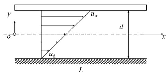
Figure 3.
Plate shear flow. Here, is the plate length, is the plate distance and and are the speed of upper and lower plates.
Similar to Couette flow, a general expression of hard constraints is formulated, i.e.,
3.2.1. Effect of Degree
According to Equation (23), three hard constraints with different degrees (i.e., = 1.0, 2.0 and 3.0) and the same scaling factor (i.e., = 1.0) are generated to examine the effect of degree on the prediction accuracy of PINN for the plate shear flow.
In order to quantitatively measure the prediction accuracy of PINN for the plate shear flow, a relative L2-norm error is defined as follows, i.e.,
where is the analytic solution of axial velocity at the i-th node, and is the number of the computational node. The relative L2-norm error of axial velocity predicted by the PINN and the analytic solution at different degrees and Reynolds numbers are shown in Table 3. It can be observed that, with the increase in Reynolds number, the PINN-prediction results exhibit an increasing trend. However, across all ranges of Reynolds numbers, both second- and third-degree hard constraints result in obviously smaller relative errors than the first-degree hard constraint, despite the errors of second-degree hard constraints being slightly larger than those of third-degree ones.
Table 3.
The L2-norm errors of axial velocity of plate shear flow with different degrees of hard constraints.
Figure 4 compares the distributions of axial velocity by PINN against the analytic solution at a Reynolds number of 60.0. From the figure, significant deviations are observed for PINN-predicted results with first-degree hard constraints, while the predicted axial velocity distributions by PINNs with second- and third-order hard constraints exhibit good agreements with the analytic solutions, corresponding to the errors shown in Table 3.
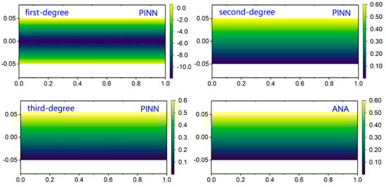
Figure 4.
Comparison of axial velocity distributions in plate shear flow between PINN-predicted results with different degrees of hard constraint and analytic solution.
3.2.2. Effect of Scaling Factor
Seven hard constraints with different magnitudes of (i.e., = 1.0 × 10⁻⁶, 1.0 × 10⁻⁴, 1.0 × 10⁻², 1.0, 1.0 × 10², 1.0 × 10⁴ and 1.0 × 10⁶) and the same degree (i.e., = 2.0) are formulated to examine the effect of scaling factor on the PINN prediction accuracy.
The relative L2-norm errors of axial velocity at different Reynolds numbers are listed in Table 4. As the values of approach 1.0, the relative L2-norm errors of axial velocity between PINN-predicted results and analytic solutions become smaller. In addition, the large values of relative L2-norm errors with = 1.0 × 10⁻⁶ and = 1.0 × 10⁶ in Table 4 are still smaller than those with first-degree hard constraints in Table 3, further demonstrating that the selection of degree is crucial to the PINN prediction accuracy.
Table 4.
The L2-norm errors of axial velocity of plate shear flow predicted by the PINN and the analytic solution at different scaling factors and Reynolds numbers.
Figure 5 further shows the axial velocity distributions at a Reynolds number of 60. The best agreement between the PINN-predicted distribution of axial velocity and the analytic solution is achieved for the case of = 1.0, corresponding to the quantitative comparison results in Table 4.
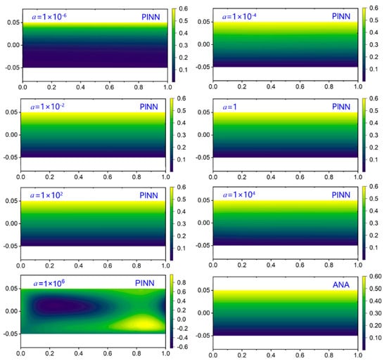
Figure 5.
Comparison of axial velocity distributions in plate shear flow between PINN-predicted results with different scaling factors and analytic solutions.
3.3. Stenotic Flow/Aneurysmal Flow
The third test example is the stenotic/aneurysmal flow of idealized flood flow, which describes vasoconstriction/dilation in biological fluid mechanics, as shown in Figure 6. The geometry of the stenotic/aneurysmal flow can be mathematically expressed as:
where is the inlet diameter before vasoconstriction or dilation, which is fixed to be 0.05; and define the shape of vasoconstriction/dilation and equal 0.5 and 0.1, respectively; is a constant that determines the degree of vasoconstriction/dilation. A positive value of corresponds to the stenotic flow while a negative value corresponds to the aneurysm flow, and a greater absolute value of A indicates a higher degree of expansion/contraction of the flow channel. In the following test, PINN-predicted results for different geometries of the flow channel (i.e., = 4.0 × 10⁻³, 7.0 × 10⁻³, − 1.2 × 10⁻² and − 2.2 × 10⁻²) are examined while the inlet and outlet pressure are set to be 0.1 and 0, respectively, and the viscosity is 1.0 × 10⁻³. Since there is no analytic solution for the investigated stenotic/aneurysmal flow, CFD simulations based on the conventional FV method are performed to provide a benchmark for the PINN-predicted results. The commercial flow solver ANSYS-Fluent is employed to conduct the FV-based CFD simulations. The second-order upwind scheme and second-order central scheme are adopted for the discretization of convection and diffusion terms, respectively, and the SIMPLE (semi-implicit method for pressure linked equations) algorithm is utilized for pressure–velocity coupling. As the Reynolds number is low and the flow is completely laminar, no turbulence model is employed in the computations. A structured computational grid with 20 × 100 cells in streamwise and vertical directions is used in the FV-based CFD simulations.
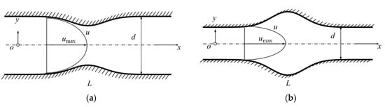
Figure 6.
Stenotic flow and aneurysmal flow: (a) stenotic flow; (b) aneurysmal flow. Here, is the channel length, is the distance between the channel walls, is the local streamwise velocity and is the velocity at the center line.
Similar to Couette flow, a general expression of hard constraints is formulated, i.e.,
3.3.1. Effect of Degree
Three hard constraints with different degrees (i.e., = 1.0, 2.0 and 3.0) and the same scaling factor (i.e., = 1.0) are generated for PINN model construction.
For stenotic/aneurysmal flow, relative L2-norm error is adopted to measure the PINN prediction accuracy, where in Equation (24) denotes the FV-based CFD-predicted axial velocity at the i-th node. The relative L2-norm errors of axial velocity with different degrees are listed in Table 5. As the pressure at the inlet and outlet is fixed and the geometric parameter A has a considerable effect on the pressure drop in the flow channel, the Reynolds number, defined with , and at the inlet of the computational domain, varies in the range of 12.5 to 18.0. For the four examined geometries, both second- and third-degree hard constraints result in smaller errors than the first-degree hard constraint. Compared with the second-degree hard constraint, the third-degree hard constraint results in slightly enhanced prediction accuracy.
Table 5.
The L2-norm errors of axial velocity of stenotic/aneurysmal flow predicted by PINN with different degrees of hard constraints.
In Figure 7 and Figure 8, the distributions of axial velocity for stenotic/aneurysmal flow are further compared between PINN and FV-based CFD. For the sake of saving space, only the results of stenotic flow with A of 4.0 × 10⁻³ and aneurysmal flow with A of −2.2 × 10⁻² are provided. There are significant deviations between PINN-predicted results with first-degree hard constraints and FV-based CFD results, while the predicted axial velocity distributions by PINNs with second- and third-degree hard constraints exhibit good agreements with the FV-based CFD results, corresponding to the errors shown in Table 5.
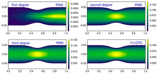
Figure 7.
Comparison of axial velocity distributions in stenotic/aneurysmal flow ( = 4.0 × 10⁻³) between PINN-predicted results with different degrees of hard constraints and FV-based CFD results.
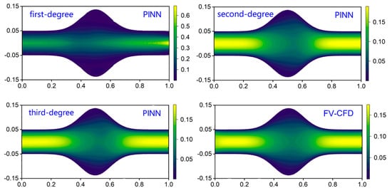
Figure 8.
Comparison of axial velocity distributions in stenotic/aneurysmal flow ( = −2.2 × 10⁻³) between PINN-predicted results with different degrees of hard constraints and FV-based CFD results.
3.3.2. Effect of Scaling Factor
Similar to the previous tests, five hard constraints with different magnitudes of (i.e., = 1.0 × 10⁻⁴, 1.0 × 10⁻², 1.0, 1.0 × 10² and 1.0 × 10⁴) and the same degree (i.e., = 2.0) are formulated. The relative L2-norm errors of the axial velocity predicted by PINN and FV-based CFD in the cases of = 4.0 × 10⁻³, = 7.0 × 10⁻³, = −1.2 × 10⁻² and = −2.2 × 10⁻² are listed in Table 6. Relative small errors are observed to be achieved when the scaling factor varies between 1.0 × 10⁻² and 1.0 × 10², while the errors tend to become unacceptable when becomes even smaller or larger, i.e., = 1.0 × 10⁻⁴ and = 1.0 × 10⁴. In addition, the relatively large errors with = 1.0 × 10⁻⁴ and = 1.0 × 10⁴ in Table 6 are still smaller than those with first-degree hard constraints in Table 5, further demonstrating the importance of degree in the PINN prediction accuracy.
Table 6.
Relative errors of axial velocity of stenotic flow/aneurysmal flow predicted by PINN and FV-based CFD results at different scaling factors.
The contours of axial velocity distributions are shown in Figure 9 and Figure 10. For = 1.0, although the L2-norm error is slightly larger than those with = 1.0 × 10⁻² and = 1.0 × 10² (Table 6), the axial velocity distributions in the local stenotic/aneurysmal part are observed to best agree with the FV-based CFD result.
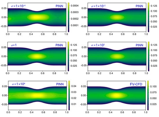
Figure 9.
Comparison of axial velocity distributions in stenotic flow ( = 4.0 × 10⁻³) between PINN-predicted results with different scaling factors and FV-based CFD results.
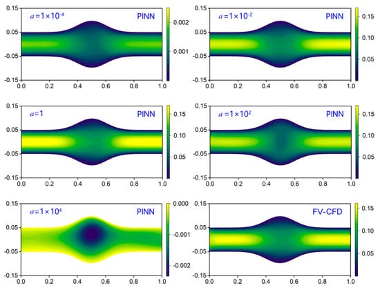
Figure 10.
Comparison of axial velocity distributions in aneurysmal flow ( = −1.2 × 10⁻²) between PINN-predicted results with different scaling factors and FV-based CFD results.
In summary, the degree of the smooth function of the hard constraint has the most impact on PINN-predicted results, followed by the scaling factor. Specifically, when the degree is 2.0 or 3.0, the PINN-predicted results exhibit a relatively high level of agreement with the analytic solutions or FV-based CFD results. However, when the degree is reduced to 1.0, there are significant deviations between PINN-predicted results and analytic solutions or FV-based CFD results. This is because the first-degree hard constraint may lead to a value of 0.0 for the second derivative term in the loss function shown in Equation (8), which is inconsistent with physical reality. From this point of view, the degree of the constraint expression should be at least two. In addition, selecting a scaling factor that is either too large (e.g., 1.0 × 10⁴) or too small (e.g., 1.0 × 10⁻⁴) can amplify or reduce the impact of network output (i.e., , ) on the final solution (i.e., , ), giving rise to large errors. The scaling factor of the hard constraint is recommended to be around 1.0.
4. Conclusions
In the present work, the PINN-based solving method for Navier–Stokes equations with hard constraints is implemented in Couette flow, plate shear flow and stenotic/aneurysmal flow at various Reynolds numbers. Particular efforts are devoted to investigating the effects of two parameters embedded in the smooth function of the hard constraints, i.e., the degree and the scaling factor, on the prediction accuracy. The following principles for the hard constraint formulation are derived from the numerical test results. First, the degree of the constraint has a significant impact on the prediction accuracy, and it should be at least two. Increasing the degree from two to three may lead to a larger prediction error. Second, it is recommended that the scaling factor of the constraint should be maintained around 1.0. Altering it to 1.0 × 10⁻² or 1.0 × 10² may elevate the sensitivity of prediction results to variations in the Reynolds number.
This work may promote our understanding of the PINN method in solving partial differential equations, and the guidelines derived for the hard constraint method may provide references for the development of PINN methods. Despite the inspiring results in this research, the solving scope of the present hard constraint method for PINN is limited to flow problems with regular domain topology. In follow-up studies, more efforts should be devoted to developing a more sophisticated hard constraint and expanding the applicability of the PINN method, especially in addressing complex flow problems such as separated flows, compressible flows and even turbulent flows.
Author Contributions
Conceptualization, Y.J. and C.Z.; methodology, Z.X., Y.J., Z.L. and J.Z.; software, Z.X.; validation, Z.X. and J.Z.; formal analysis, Z.X.; investigation, Z.X., Y.J. and Z.L.; resources, Y.J. and C.Z.; data curation, Z.X.; writing—original draft preparation, Z.X.; writing—review and editing, Y.J., Z.L. and C.Z.; visualization, Z.X.; supervision, Y.J. and C.Z.; project administration, Y.J. and C.Z.; funding acquisition, Y.J. and C.Z. All authors have read and agreed to the published version of the manuscript.
Funding
This work was supported by the State Key Laboratory for Strength and Vibration of Mechanical Structures Project of China under Grant No. SV2021-ZZ-23.
Institutional Review Board Statement
Not applicable.
Informed Consent Statement
Not applicable.
Data Availability Statement
The data that support the findings of this study are available from the corresponding author upon reasonable request.
Conflicts of Interest
The authors declare no conflict of interest.
References
- Slotnick, J.; Khodadoust, J.; Alonso, J.; Darmofal, D.; Gropp, W.; Lurie, E.; Mavriplis, D. CFD Cision 2030 Study: A Path to Revolutionary Computational Aerosciences; NASA Technical Report NASA/CR-2014-218178; NASA Langley Research Center: Hampton, VA, USA, 2014. [Google Scholar]
- Houzeaux, G.; Garcia-Gasulla, M. High performance computing techniques in CFD. Int. J. Comput. Fluid Dyn. 2022, 34, 457. [Google Scholar] [CrossRef]
- Lagaris, I.E.; Likas, A.; Fotiadis, D.I. Artificial neural networks for solving ordinary and partial differential equations. IEEE Transact. Neural Netw. 1998, 9, 987–1000. [Google Scholar] [CrossRef]
- Brenner, M.P.; Eldredge, J.D.; Freund, J.B. Perspective on machine learning for advancing fluid mechanics. Physic. Rev. Fluids 2019, 4, 100501. [Google Scholar] [CrossRef]
- Rabault, J.; Kuchta, M.; Jensen, A.; Réglade, U.; Cerardi, N. Artificial neural networks trained through deep reinforcement learning discover control strategies for active flow control. J. Fluid Mech. 2019, 865, 281–302. [Google Scholar] [CrossRef]
- Wu, M.Y.; Wu, Y.; Yuan, X.Y.; Chen, Z.H.; Wu, W.T.; Aubry, N. Fast prediction of flow field around airfoils based on deep convolutional neural network. Appl. Sci. 2022, 12, 12075. [Google Scholar] [CrossRef]
- Pham-Sy, N.; Tran, C.D. Parallel computation using non-overlapping domain decomposition coupled with compact local integrated RBF for Navier–Stokes equations. Int. J. Comput. Fluid Dyn. 2022, 36, 835–856. [Google Scholar] [CrossRef]
- Ju, Y.P.; Qin, R.H.; Kipouros, T.; Parks, G.; Zhang, C.H. A high-dimensional design optimisation method for centrifugal impellers. Proc. Inst. Mech. Eng. Part A J. Power Energy 2016, 230, 272–288. [Google Scholar] [CrossRef]
- Hu, H.; Yu, J.; Song, Y.; Chen, F. The application of support vector regression and mesh deformation technique in the optimization of transonic compressor design. Aerosp. Sci. Technol. 2021, 112, 106589. [Google Scholar] [CrossRef]
- Qin, R.H.; Ju, Y.P.; Galloway, L.; Spence, S.; Zhang, C.H. High dimensional matching optimization of impeller–vaned diffuser interaction for a centrifugal compressor stage. J. Turbomach. 2020, 142, 121004. [Google Scholar] [CrossRef]
- Balajewicz, M.J.; Dowell, E.H.; Noack, B.R. Low-dimensional modelling of high-Reynolds-number shear flows incorporating constraints from the Navier–Stokes equation. J. Fluid Mech. 2013, 729, 285–308. [Google Scholar] [CrossRef]
- Ba, Z.; Wang, Y. Numerical analysis of transient state heat transfer by spectral method based on POD reduced-order extrapolation algorithm. Appl. Sci. 2023, 13, 6665. [Google Scholar] [CrossRef]
- Cai, S.; Mao, Z.; Wang, Z.; Yin, M.; Karniadakis, G.E. Physics-informed neural networks (PINNs) for fluid mechanics: A review. Acta Mech. Sin. 2021, 37, 1727–1738. [Google Scholar] [CrossRef]
- Raissi, M.; Perdikaris, P.; Karniadakis, G.E. Physics-informed neural networks: A deep learning framework for solving forward and inverse problems involving nonlinear partial differential equations. J. Comput. Phys. 2019, 378, 686–707. [Google Scholar] [CrossRef]
- Guo, Y.; Cao, X.; Liu, B.; Gao, M. Solving partial differential equations using deep learning and physical constraints. Appl. Sci. 2020, 10, 5917. [Google Scholar] [CrossRef]
- Mao, Z.; Jagtap, A.D.; Karniadakis, G.E. Physics-informed neural networks for high-speed flows. Comput. Methods Appl. Mech. Eng. 2020, 360, 112789. [Google Scholar] [CrossRef]
- Raissi, M.; Yazdani, A.; Karniadakis, G.E. Hidden fluid mechanics: Learning velocity and pressure fields from flow visualizations. Science 2020, 367, 1026–1030. [Google Scholar] [CrossRef] [PubMed]
- Sun, L.; Gao, H.; Pan, S.; Wang, J.X. Surrogate modeling for fluid flows based on physics-constrained deep learning without simulation data. Comput. Methods Appl. Mech. Eng. 2020, 361, 112732. [Google Scholar] [CrossRef]
- Jin, X.; Cai, S.; Li, H.; Karniadakis, G.E. NSFnets (Navier-Stokes flow nets): Physics-informed neural networks for the incompressible Navier-Stokes equations. J. Comput. Phys. 2021, 426, 109951. [Google Scholar] [CrossRef]
- Jagtap, A.D.; Kawaguchi, K.; Karniadakis, G.E. Adaptive activation functions accelerate convergence in deep and physics-informed neural networks. J. Comput. Phys. 2020, 404, 109136. [Google Scholar] [CrossRef]
- Wang, S.; Teng, Y.; Perdikaris, P. Understanding and mitigating gradient flow pathologies in physics-informed neural networks. SIAM J. Sci. Comput. 2021, 43, A3055–A3081. [Google Scholar] [CrossRef]
- Karniadakis, G.E.; Jagtap, A.D. Extended physics-informed neural networks (XPINNs): A generalized space-time domain decomposition based deep learning framework for nonlinear partial differential equations. Commun. Comput. Phys. 2020, 28, 2002–2041. [Google Scholar] [CrossRef]
- Márquez-Neila, P.; Salzmann, M.; Fua, P. Imposing hard constraints on deep networks: Promises and limitations. arXiv 2017, arXiv:1706.02025. [Google Scholar]
- Baydin, A.G.; Pearlmutter, B.A.; Radul, A.A.; Siskind, J.M. Automatic differentiation in machine learning a survey. J. Mach. Learn. Res. 2018, 18, 1–43. [Google Scholar]
- Ramachandran, P.; Zoph, B.; Le, Q.V. Searching for activation functions. arXiv 2017, arXiv:1710.05941. [Google Scholar]
- Kingma, D.P.; Ba, J. Adam: A method for stochastic optimization. arXiv 2014, arXiv:1412.6980. [Google Scholar]
- He, K.; Zhang, X.; Ren, S.; Sun, J. Delving Deep into Rectifiers: Surpassing Human-level Performance on ImageNet Classification. In Proceedings of the 2015 IEEE International Conference on Computer Vision, Santiago, Chile, 7–13 December 2015. [Google Scholar]
- Dehal, R.S.; Munjal, C.; Ansari, A.A.; Kushwaha, A.S. GPU Computing Revolution: CUDA. In Proceedings of the 2018 International Conference on Advances in Computing, Communication Control and Networking, Greater Noida, India, 12–13 October 2018. [Google Scholar] [CrossRef]
- Paszke, A.; Gross, S.; Massa, F.; Lerer, A.; Bradbury, J.; Chanan, G.; Killeen, T.; Lin, Z.; Gimelshein, N.; Antiga, L.; et al. PyTorch: An Imperative Style, High-performance Deep Learning Library. In Proceedings of the 33rd International Conference on Neural Information Processing Systems, New York, NY, USA, 8–14 December 2019. [Google Scholar]
Disclaimer/Publisher’s Note: The statements, opinions and data contained in all publications are solely those of the individual author(s) and contributor(s) and not of MDPI and/or the editor(s). MDPI and/or the editor(s) disclaim responsibility for any injury to people or property resulting from any ideas, methods, instructions or products referred to in the content. |
© 2024 by the authors. Licensee MDPI, Basel, Switzerland. This article is an open access article distributed under the terms and conditions of the Creative Commons Attribution (CC BY) license (https://creativecommons.org/licenses/by/4.0/).