Abstract
Aiming to serve as a preliminary study for South Korea’s national GHG emission factor development, this study reviewed data treatment and sample size determination approaches to establishing the destruction and removal efficiency (DRE) of the semiconductor and display industry. We used field-measured DRE data to identify the optimal sample size that can secure representativeness by employing the coefficient of variation and stratified sampling. Although outlier removal is often a key process in the development of field-based coefficients, it has been underexplored how different outlier treatment options could be useful when data availability is limited. In our analysis, three possible outlier treatment cases were considered: no treatment (using data with outliers as they are) (Case 1), outlier removal (Case 2), and adjustment of outliers to extreme values (Case 3). The results of the sample size calculation showed that a minimum of 17 and a maximum of 337 data (out of a total of 2968 scrubbers) were required for determining a CF4 gas factor and that a minimum of 3 and a maximum of 45 data (out of a total of 2917 scrubbers) were required for determining a CHF3 gas factor. Our findings suggest that (a) outlier treatment can be useful when the coefficient of variation lacks information from relevant data, and (b) the CV method with outlier adjustment (Case 3) can provide the closest result to the sample size resulting from the stratified sampling method with relevant characteristics considered.
1. Introduction
In October 2020, South Korea declared to achieve carbon neutrality by 2050. In December 2021, the country submitted a strengthened nationally determined contribution to greenhouse gas (GHG) reduction (40% reduction from the total GHG emissions of 727.6 million tons CO2eq in 2018 by 2030) to the United Nations Framework Convention on Climate Change in response to the Paris Agreement. In March 2023, the Korean government released the First National Carbon Neutrality and Green Growth Master Plan (Government Draft), which details specific sectoral and annual GHG reduction targets to be achieved by 2030 [1].
The industrial sector is one of the major greenhouse gas emitters in South Korea, with the semiconductor and display industry being a significant contributor. The semiconductor and display industry generates GHGs primarily via the use of electricity and fluorinated GHGs in etching and deposition processes. As of 2020, greenhouse gas emissions from the semiconductor and display industry amounted to approximately 20 million tons of CO2eq, and this emission trend has been on the rise due to the increasing demand for semiconductors and technological advancements [2]. In response, Korean semiconductor and display industries are making various efforts to reduce GHG emissions, one of which was the launch of a public–private partnership called the Semiconductor and Display Carbon Neutrality Committee [3].
In South Korea, the estimation of GHG emissions from the semiconductor and display industry relies on Tier 2a and 2b methods proposed in the Intergovernmental Panel on Climate Change (IPCC) guidelines and the IPCC default values. Among the parameters for calculating GHG emissions, the volume fraction of gas and the residual percentage of gas in Bombe are applied to the data of the business site when available. The IPCC default values are applied if there is no data available at the business site [4,5,6].
In the context of our study, destruction and removal efficiency (DRE) refers to the efficiency of scrubbers in reducing greenhouse gas emissions in the semiconductor and display industry. The IPCC coefficient for each type of greenhouse gas is averaged over the characteristics of the target scrubber. The IPCC guidelines recommend using country-specific values to calculate GHG emissions as a way to improve inventory reliability. However, South Korea is currently using the IPCC default values for the sector’s DRE due to the absence of country-specific estimates.
In the case of South Korea, only a limited number of business sites calculate GHG emissions by applying the values estimated by themselves. To improve the reliability of the GHG inventories, it is ideal to develop national GHG emission factors based on an exhaustive survey of on-site data. However, conducting a comprehensive survey for all business sites is practically infeasible due to physical and time constraints. The determination of a reliable DRE for each type of GHG with limited data requires rigorous statistical approaches to optimizing the sample size and treating outliers effectively. This is especially the case for semiconductor and display industries, considering that there are various types of GHGs (about 11 types, including PFCs and HFCs) and a large number of scrubbers (more than 3000).
Aiming as a preliminary study for the development of South Korea’s national GHG emission factors, the present study explores different approaches to determining the optimal number of samples and processing them so the sampled data can be representative of the population. To this end, we review sampling methods, examine data processing approaches, and evaluate the applicability of each case.
2. Review of Sampling Methods
Developing the national emission factors typically involves a comprehensive survey, which is the best method, but can be time-consuming and costly. An alternative approach to address these problems is to collect a representative sample. A sample is an actual measurement obtained from a population, a set of units extracted from a sampling frame, and a subset of the population. A sample must resemble the population to enable the estimation of the parameter that is a characteristic of the population. A study with an underestimated sample size will not have sufficient power, rendering the results of the study unreliable. On the other hand, an overestimated sample size makes it challenging to prove the significance of the results even though the results may have substantial power. Calculating the sample size, therefore, requires various pieces of information to be considered, including the effective sample size, significance level, power, and variability, which are considered parameters [7,8,9,10,11]. Using parameter estimates in sample size calculation requires introducing uncertainty into the sample size itself. Therefore, in this study, we investigated various possible ways to extract a sample and proceeded with the most suitable method.
2.1. Sample Size Determination through Stratified Sampling
Among different sampling methods, the probability sampling method allows the generalization of analysis results through random sampling [12,13,14]. Stratified sampling is one type of probability sampling methods. The stratified sampling method has the advantage of increasing the representativeness of the sample through stratification, facilitating its population representativeness and the identification of the characteristics via stratum. However, the downside of having prior knowledge of the population is that more information is required for stratification, and if the stratification is too complex or erroneous, sampling errors can increase [15,16,17]. The stratified sampling method distributes the sample in four ways, which are detailed in Table 1.

Table 1.
Stratified Sampling Methods.
2.2. Sample Size Determination through Cluster Sampling
Cluster sampling involves classifying a population into several small groups (clusters), randomly selecting a predetermined number of small groups from the clusters, and sampling from the selected groups through simple random sampling. Because cluster sampling does not sample all clusters but only a subset of them, there is a risk of selecting a biased sample if the clusters are internally homogeneous. In cluster sampling, for this reason, clusters must be heterogeneous within and homogeneous across clusters, unlike stratified sampling [18,19,20].
When organizing clusters, the size of each cluster should be as similar as possible to ensure that the size of the cluster is set at an appropriate level for control, and consideration should be given to reducing the on-site survey time and cost. This can be achieved by selecting a small number of clusters and taking many samples from each or selecting a large number of clusters and taking a few samples from each. The choice between these two depends on which method is more efficient in terms of the survey time and cost. Cluster sampling divides the population into multiple clusters and extracts the required number of clusters through simple random sampling. These selected clusters are then used as a procedure to construct a sample from the elements within the extracted clusters.
Yang (2022) conducted a study responding to the heightened demand for the analysis of sensor multivariate data in manufacturing settings driven by advancements in sensor technology. The research involved performing hierarchical clustering analysis based on distance correlation coefficients using process data that included binary outcomes, such as pass/fail decisions. The primary objective was to investigate the potential independence among independent variables by grouping sensors exhibiting high correlation into a unified entity [21]. Qing et al. (2021) delved into the challenges of estimating population parameters for various ecological indicators, such as forest area, productivity, and biodiversity, within forest ecosystems. To enhance the precision of these estimations, the study explored the utility of generalized systematic adaptive cluster sampling as a remedy to the limitations associated with systematic adaptive cluster sampling. The research aimed to improve the accuracy of estimating population parameters for diverse ecological metrics in forest ecosystems [22].
2.3. Using the Coefficient of Variation for Sample Size Determination
If some relevant information about the population is known, a sample can be extracted using confidence levels, margins of error, and coefficients of variation. The Korea Energy Agency (KEA) introduced a sampling method using a coefficient of variation (CV) in their “M&V Guidelines for Calculating Energy Savings for Equipment Replacement.” The sampling procedure recommended by KEA is summarized in Table 2. If previously measured information is available on the population, the CV can be calculated, and if there is no prior information on the population, the CV can be arbitrarily assigned to 0.5 [23,24,25].
Table 2.
Procedure for determining the sample size with CVs of variation and required materials.
Marcos et al. (2017) utilized the CV method to establish an optimal sample size, ensuring the representativeness and validity of the research outcomes before embarking on experiments to estimate characteristics of four Crotalaria species [26]. Andre et al. (2021) conducted experiments to investigate the characteristics of cassava under different nursery conditions, estimating the appropriate sample size for the experiment through the assessment of the CV [27].
3. Target Gas Selection and Data Collection
DREs in the semiconductor display industry cover a wide range of F-gases. This study utilized ground truth Tier 3 DRE data to calculate the number of samples. In the case of South Korea, a Tier 3 factor must be developed for facilities that emit more than 500,000 tons CO2eq of GHGs; Tier 3 refers to a factor developed through an appropriate process test method by the business site. In the semiconductor and display industry, some companies have developed and applied DRE as Tier 3 based on actual measurements, and the values reported by them are considered reliable because they are verified by the governing body and supervisory body [28]. Therefore, this study was conducted based on the data obtained from the national organizations in charge of this field-measured material.
Because the sample size in this study considers the distribution of existing measurements, the sample size was determined for CF4 and CHF3—two gases that are frequently used in the semiconductor and display industry. Table 3 shows the total sample size of the targeted F-gases and their sampling period.
Table 3.
Collected Tier 3 DRE data content.
4. Data Processing and Sample Size Determination Methods
4.1. Data Processing Methods
When determining the sample size, it is important to consider outliers, especially when calculating measurements or representative values. In particular, when it comes to the development of national GHG emission factors, outliers should be carefully examined as they can be underestimated or overestimated [29,30]. Careful examination of outliers is imperative, especially in the absence of detailed information concerning them. This study reviews the data processing methods commonly used in previous studies on inventory development and applies various ways of outlier handling to determine the appropriate sample size.
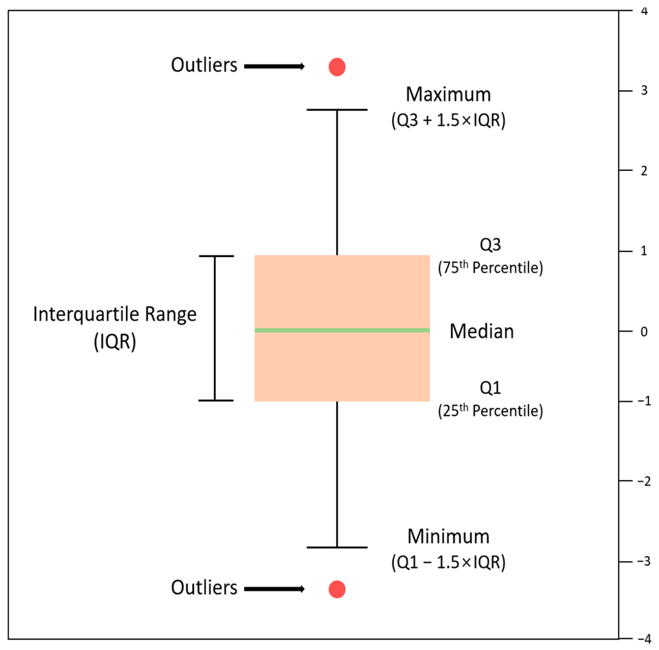
Extreme values should be identified before assuming the presence of outliers. Although several methods are available to identify extreme values, the interquartile range (IQR) method is the most popular one among them and has been used in related research. IQR identifies extreme values and finds outliers via a box-and-whisker plot, which is one of the summary methods that integrate multiple information into one figure using several measurements, such as the position of the center and degree of scatter [31,32].
From the box-and-whisker plot, you can identify most outliers in the data values in addition to the symmetry of the distribution, center of the data, degree of dispersion, and concentration of the tail of the distribution. Box-and-whisker plots are primarily built around interquartile values. A square box is drawn around 50% of the data at the center of the size-ordered data set, and lines of appropriate length are drawn and connected to the left and right (or below and above) of the box to represent the ranges of 25% of the data with smaller values and 25% of the data with larger values, respectively.
The process of IQR is as follows: First, determine the interquartile values (. Second, connect and to a square box and draw a vertical line at the position of the median (). Third, compute . Fourth, bound the box with a size range at each end and connect the minimum and maximum values within this range with lines from and , respectively. Finally, indicate the data values that fall outside the two boundaries and determine these points as extreme values. A graphical representation of the above process is shown in Figure 1.
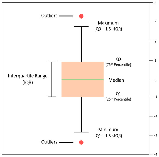
Figure 1.
Handling outliers using box-and-whisker plots.
There are different ways to handle outliers. First, you can choose to eliminate outliers to remove their influence. However, it has the disadvantage of reducing the overall number of data. Another way is to winsorize outliers. This method adjusts all values above and below the threshold set with the extreme upper and lower limits. The winsorizing method is less sensitive to outlier values because it can replace them with less extreme values [33,34]. Although estimation using winsorization introduces bias (the difference between the expected value of the estimate and the true value of the parameter), it has the advantage of reducing variance, making it more likely to be used for random sampling.
We calculated and examined the sample size for CV, based on the following three treatment optionss: using the existing data as they are (Case 1), of removing outliers (Case 2), and of adjusting outliers to extreme values (Case 3).
4.2. Sample Size Determination Methods
Here, sample size determination methods used for developing the national greenhouse gas emission factors were evaluated, including the Neyman allocation method, which is a stratified sampling method, and sample size determination method, which is based on the coefficient of variation (CV) used by the International Organization for Standardization (ISO) and Korean national organizations.
Here,
n: Total number of sample business sites
N: Number of population business sites
S: Standard deviation per stratum
h: Subscript for strata (energy sources and facilities)
D:
B: Margin of error
za/2:The value of a standard normal distribution with a confidence level of (1 − α) (with a 95% confidence level, this would be approximately 1.96).
In the method of determining the sample size using the CV, the sample size is first calculated based on the CV of the existing measured data, and the method is based on the assumption that the CV of the existing measured data is known. This method suggests that a figure of 0.5 can be utilized when there is no prior information about the target. However, in this method, having information on the existing population helps to determine the sample size of the population more accurately. The method for determining the sample size using the CV is shown in Equation (2).
Here,
n0: Initial sample size
CV: Coefficient of variation
e: Precision
za/2: (1 − α) Confidence coefficient below 100% confidence level
If N/n < 20, correct according to Equation (3).
Here,
n: Sample size
N: Total population size
In this study, we approached the sample size determination from two perspectives. Concerning the CV method, the CV information available on the existing measurement data was sufficient to calculate the sample size; hence, we chose this method, assuming that the relevant information is unknown. Additionally, in this method, we considered details about outlier handling. This method requires careful examination, especially when there is no prior information; therefore, we handled outliers under the assumption that there was no prior information and then reviewed the suitability of outlier handling based on prior information for validation.
For stratified sampling, there must be information about the data to be stratified so that the relevant data must be identifiable. In the case of stratified sampling, stratification was performed using the data related to scrubber types that can be obtained further in this study. For this study, technical information on scrubbers was obtained by surveying companies that use the gas and requesting data from relevant organizations. Because there was some prior information in this case and the number of data reduced considerably when divided into scrubber types, it is suggested that there would be difficulties in interpreting the results to apply the outlier handling method. Hence, the relevant part was not considered.
5. Results and Discussion
5.1. Results of Outlier Handling and Sample Size Determination Using Coefficient of Variation (CV)
This study used the CV to determine the target sample size for the Tier 3 DRE data in the semiconductor and display industry. The underlying assumptions were as follows. To determine the sample size using the CV, the significance and confidence levels need to be determined. For the significance level, a conservative 1% level was chosen for this study, rather than the typical 10% applied in general surveys. As for the confidence level, it was based on the most commonly used 95% confidence level. For outliers, we used IQR to find the extreme values and then calculated the sample size with no handling of outliers (Case 1), with outliers removed (Case 2), and with outliers adjusted to extreme values (Case 3).
5.1.1. Outlier Handling and Sample Size Determination for CF4 Tier 3 DRE Data
For CF4 gas, 44 Tier 3 DRE data were used, and the sample size was determined after handling outliers in each case (Table 4). The value corresponding to the third quartile (Q3) of the CF4 gas DRE values was found to be 0.969, while the value corresponding to the first quartile (Q1) was found to be 0.924. IQR for Q3 minus Q1 was found to be 0.046, while the figure considering 1.5 times the IQR was found to be 0.069. Taking these values into account, the DRE values for CF4 gas were determined as outliers if they were higher than 1.039 or lower than 0.856.
Table 4.
Resources for handling outliers in CF4 Tier 3 DREs.
The results of the Tier 3 DRE values for CF4 gas according to the case of outlier handling are shown in Table 5. In Case 1, where existing data were used, the mean was 0.921, which is the lowest among all the three cases, and the standard deviation was the highest. In Case 2, where outliers were removed, the sample size decreased by eight compared to the original; here, the mean was 0.961, which is the highest, while the standard deviation was 0.020, which is the lowest. In Case 3, where outliers were adjusted to extreme values, the mean and standard deviation values were at intermediate levels for Case 1 and Case 2.
Table 5.
DRE values for CF4 gas based on outlier cases.
For validation, we checked the characteristics of the handled outliers. The characteristic information of the current data is scrubber, and all eight of the handled outliers had burn-type attributes. Therefore, we checked the difference in outliers by including only burn-type scrubbers in the CF4 Tier 3 DRE values (Table 6).
Table 6.
Requirements for handling outliers in the Burn scrubber Tier 3 DRE during CF4.
For the CF4 gas DRE values, Q3 was found to be 0.938, while Q1 was 0.775 when including only the burn-type scrubbers. IQR for Q3 minus Q1 was 0.163, while the figure considering 1.5 times the IQR was 0.244. Based on these values, the DRE values for burn-type scrubbers in CF4 gas were considered as outliers if they exceeded 1.182 or were less than 0.531.
After applying the outlier criteria to review the DRE values obtained for the burn-type scrubber, it was found that none of the values met the outlier criteria. The mean value of the CF4 burn-type DREs was 0.843 (which is lower than the overall mean value of CF4 DREs), and their standard deviation was relatively large at 0.115 (which is within the characteristic range of CF4 burn type). This result indicates that there were no outliers that were handled. It also suggests that differences may occur depending on the presence of information about the scrubber type when processing DRE data. Due to the limitations existing in collecting relevant information from the perspective of data processing, we assume that there is no prior information on the relevant data and determine the sample size based on data processing and CV distribution.
Based on the outlier criteria, the sample size of CF4 DREs was determined using CV values, and the results are shown in Table 7. Based on the outlier criteria, the sample size was 337 for Case 1, 17 for Case 2, and 85 for Case 3. These results show that Cases 2 and 3 had relatively smaller sample sizes compared to Case 1, as outliers were treated and adjusted.
Table 7.
Sample size for CF4 DRE development considering outlier cases and CVs.
5.1.2. Outlier Handling and Sample Size Calculation for CHF3 Tier 3 DRE Data
For CHF3 gas, 39 Tier 3 DREs were used, and the sample size was determined after handling outliers in each case (Table 8). The value corresponding to Q3 of the CHF3 gas DRE values was found to be 0.999, while the value corresponding to Q1 was 0.987. IQR for Q3 minus Q1 was found to be 0.013, while the figure considering 1.5 times the IQR was found to be 0.019. Considering these values, the DRE values for CHF3 gas were judged to be outliers if they were higher than 1.019 or lower than 0.967.
Table 8.
Resources for handling outliers in CHF3 Tier 3 DREs.
Results of the Tier 3 DRE values for CHF3 gas based on the case with outlier handling are shown in Table 9. Case 1, which used existing data, had the lowest mean of 0.985 and the largest standard deviation. Case 2, which removed the outliers, had five fewer samples than before; here, the obtained mean was the highest among all three cases (0.995), and the standard deviation was the lowest (0.008). Case 3, which adjusted outliers to extreme values, had mean (0.993) and standard deviation (0.012) values that are in between those obtained for Case 1 and Case 2.
Table 9.
DRE value for CHF3 gas according to the outlier case.
For CHF3, we also checked the characteristics of the handled outliers for validation purposes. The characteristic information of the current data is scrubber, and in the case of CHF3, all five of the handled outliers had burn-type attributes. Therefore, we checked the difference between outliers in the CHF3 Tier 3 DRE values by only including burn-type scrubbers.
Of the CHF3 gas DRE values, Q3 was found to be 0.99, and Q1 was found to be 0.954 when only the burn-type scrubber was considered. IQR for Q3 minus Q1 was found to be 0.046, while the figure considering 1.5 times the IQR was found to be 0.069. Considering these values, for CHF3 gases, the burn-type DRE values above 1.068 or below 0.089 were judged as outliers.
When reviewing the DRE values for the burn type using the outlier criteria, two values were found to be outliers, which were lower than the four outliers obtained for CHF3 (Table 10). This is because the mean of the burn-type scrubber for CHF3 was 0.967, and the standard deviation was 0.051, which is relatively not much larger than the standard deviation of the burn type for CF4, so the DRE values for CHF3 were found to include some outliers as well. However, even in this case, the criteria for handling outliers can vary depending on whether the scrubber has information or not, indicating that much attention is needed to handle outliers. Thus, we believe that relatively more information is needed to handle outliers in F-gas.
Table 10.
Requirements for handling outliers in the Burn scrubber Tier 3 DRE during CHF3.
To determine the sample size for the CHF3 DRE development, CV values based on the outlier criteria were used, and the results are presented in Table 11. According to the outlier criteria, the sample size calculated was 45 for Case 1, 3 for Case 2, and 6 for Case 3. These results show that Cases 2 and 3 had relatively smaller sample sizes than Case 1, as outliers were treated and adjusted. For CHF3 DRE, the required sample size is lower than that required for CF4 DRE because CHF3 data are more homogeneously distributed than CF4 data, as seen in the outlier handling process.
Table 11.
The sample size for CHF3 DRE development considering outlier cases and CVs.
5.2. Sample Size Calculation Using the Neyman Allocation Method
Among the various stratified sampling methods, the number of DRE samples was determined according to Neyman allocation, assuming that there is sufficient relevant information for stratification. Because the data available for this study are scrubber type, the sample size for developing DRE for CF4 and CHF3 gases was determined by considering the scrubber type and total population count.
5.2.1. Sample Size Calculation for CF4 Tier 3 DRE Using the Neyman Allocation Method
In this study, the total number of scrubbers required for the Tier 3 development of target gas was obtained to confirm the information related to the population. The number of CF4 scrubbers, considering scrubber types, is presented in the following Table 12.
Table 12.
Number of scrubbers by scrubber type for DRE development in CF4.
To stratify and calculate the sample size using Neyman allocation, information regarding the standard deviation for the characteristic of the substance in each stratum is required in addition to the stratum population. Because the purpose of this study was to identify the sample size for developing the DRE values, the mean and standard deviation of Tier 3 DRE for CF4 gas by scrubber type were determined and presented in Table 13.
Table 13.
Tier 3 DRE mean and standard deviation by scrubber type in CF4.
The results of DRE calculations by scrubber type indicate that the plasma type had the highest value at 0.970, followed by the catalytic type at 0.945, and the burn type had the lowest value at 0.768, along with the largest standard deviation.
The calculation of the sample size using Neyman allocation considered the same error level (1%) and confidence level (95% confidence interval) as the previous method of calculating the sample size using CV. The sample size was calculated according to Neyman allocation considering the characteristics (standard deviation) of the strata, and the sample size per stratum is shown in Table 14 considering the proportion of the population in each stratum. After calculating the sample size, it was found that a total of 21 samples were required for the development of CF4 DRE, with two burn types, 18 plasma types, and one catalyst type by stratum.
Table 14.
Number of samples per scrubber type for CF4 DRE development considering the Neumann distribution method.
5.2.2. Sample Size Calculation for CHF3 Tier 3 DRE Using the Neyman Allocation Method
In this study, the total number of scrubbers required for the Tier 3 development of target gases was obtained to confirm the information related to the population. The number of CHF3 scrubbers, considering scrubber types, is presented in the following Table 15.
Table 15.
Number of scrubbers per scrubber type for DRE development in CHF3.
For CHF3, the standard deviation is also required to understand the stratum characteristics. Therefore, the mean and standard deviation of Tier 3 DRE for CHF3 gas by scrubber type were calculated and presented in the table.
The results of the DRE calculations by scrubber type for CHF3 show that the plasma type had the highest value at 0.996, followed by the catalytic type at 0.986, and the burn type had the lowest value at 0.967, along with the highest standard deviation (Table 16).
Table 16.
Tier 3 DRE mean and standard deviation by scrubber type in CHF3.
In the case of CHF3, the determination of the sample size using Neyman allocation considered the same error level (1%) and confidence level (95% confidence interval) as the previous method of estimating the sample size using CV. The sample size was calculated according to Neyman allocation considering the characteristics (standard deviation) of the strata, and the sample size per stratum is shown in Table 17 considering the proportion of the population in each stratum. The sample size determination revealed that a total of six samples were required to develop a DRE for CHF3, with one burn type, four plasma types, and one catalyst type per layer.
Table 17.
Number of samples per scrubber type for CHF3 DRE development considering the Neumann distribution method.
5.3. Comparison of Sample Sizes Based on Determination Methods and Criteria
To consider various conditions, the sample size in this study was determined using two methodologies: CV, which can be used only when the measured value information for the measured object is known, and Neyman allocation, which can be used when there is enough information to divide the strata. In the CV method, details related to data processing must be considered when there is no prior information, so we considered the data processing case as well. The target gases are CF4 and CHF3, which are F-gases used in the semiconductor and display industry.
Table 18 shows a comparison of sample sizes by method of determination. It was found that to develop the DRE of CF4 gas, the CV method, which uses existing data as they are without handling outliers, required a sample size of 337. Case 3 required 85 samples, while the Neyman allocation method required 21 samples and 17 samples for Case 2. For CHF3, we found that Case 1 required the highest sample size of forty-five, followed by Case 3 in the CV method and the Neyman allocation method, which both required six samples, while Case 2 required the lowest with three samples, similar to CF4. These findings indicate that outlier removal considerably reduces the variance between measurements, suggesting that a smaller sample is needed overall. However, caution should be exercised when removing outliers, as valid data should not be removed inadvertently. For Case 3, CHF3 is similar to the sample size by Neyman allocation, and for CF4, the sample size determined by Neyman allocation is less than Case 3 but larger than Case 2. Therefore, adjusting outliers to extreme values might be a better approach than their complete removal when processing data.
Table 18.
Sample size for CHF3 DRE development considering outlier cases and CVs.
6. Conclusions
As preliminary research for developing Korea’s national DREs in the semiconductor and display industry, the present study aimed to review different determination methods for sample size and data processing. To this end, we examined different sample size calculation methods and selected two methods. For analysis, measurement-based DRE data were obtained for CF4 and CHF3, which are the two gases utilized in the semiconductor and display industry, and were used to calculate the minimum and maximum sample sizes. Some of the previous studies employed the CV method to develop Korea’s national GHG emission factors whereas others applied the stratified sampling method. In this study, we employed both methods. The CV method can be considered for many situations; for example, when prior information is unknown, we can apply different ways to handle outliers. In our study, the treatment of outliers was examined in three different ways—using the existing data as they are (Case 1), removing outliers (Case 2), and adjusting outliers to extreme values (Case 3)—because the choice of outlier handling method can influence the results of sample size calculations.
Depending on the determination method applied, we obtained different optimal sample sizes as follows. For the development of CF4 gas DRE, it turned out that a minimum of 17 and a maximum of 337 data points needed to be collected out of a total of 2968 scrubber data. For CHF3, a minimum of three and a maximum of 45 data points were required out of a total of 2917 scrubber data. The number of samples calculated by the Neumann distribution method, which reflects the scrubber characteristics of the sample, was close to the result of Case 3. In this regard, using a CV and adjusting the outliers (Case 3) can be one of the most feasible ways to reflect the scrubber characteristics when there is no detailed information about the business site.
For CF4 and CHF3 gas DREs, plasma-type scrubbers were found to be outliers due to the large variation exhibited by them in the data. As there are limited data that can be removed as outliers on an individual plasma-type basis, eliminating outliers could be challenging in applying a CV to calculate the sample size. When outliers were adjusted to extreme values, the sample size characterizing the scrubber was equal to or slightly higher than the result of outlier removal, indicating that the Case 3 method is likely to be more reliable than removing outliers when they must be handled. It is also regarded that the scrubber type needs to be considered when developing DRE factors for the semiconductor and display industry. This is because the DRE for this industry currently provided by the IPCC is offered only in an overall mean value without consideration of scrubber type.
It is important to note the limitations of this study. Due to the lack of prior information, we could consider only the scrubber characteristics in our analysis. Also, it will be important in future work to examine the validation methodology beyond the sample size calculation. We believe these limitations can be addressed in a future study with a larger sample size and more empirical data.
Nevertheless, the findings of our study offer important contributions. The results relating to scrubber types highlight the errors that can be introduced by other methods that currently do not take scrubber types into account. In particular, some scrubber types including burn-, heat-, and plasma-type scrubbers can be seen as outliers when compared to the overall average. In this respect, the present study demonstrates the need to consider scrubber type in the development of gas-specific national DREs. The development of a representative national DRE can be further strengthened by applying a validation method to the calculated sample size and a relevant methodology for the various gases utilized in the semiconductor and display industry.
Author Contributions
Their contributions are presented below. Conceptualization, D.M.; Writing—original draft, S.K.; Data curation, J.W.; Methodology, E.-c.J.; Formal analysis, J.L. All authors have read and agreed to the published version of the manuscript.
Funding
This work was supported by the Korea Environment Industry & Technology Institute (KEITI) through “Climate Change R&D Project for New Climate Regime”, funded by the Korea Ministry of Environment (MOE) (No. 2022003560008).
Institutional Review Board Statement
Not applicable.
Informed Consent Statement
Not applicable.
Data Availability Statement
Data are contained within the article.
Conflicts of Interest
The authors declare no conflict of interest.
References
- 2050CNC (Presidential Commission on Carbon Neutrality and Green Growth) Home Page. First National Carbon Neutrality and Green Growth Basic Plan (Government Draft). Available online: https://www.2050cnc.go.kr/base/board/read?boardManagementNo=3&boardNo=1397&searchCategory=&page=1&searchType=&searchWord=&menuLevel=2&menuNo=17 (accessed on 19 April 2023).
- GIR (Greenhouse Gas Inventory and Research Center). 2022 National Greenhouse Gas Inventory Report (2023); Greenhouse Gas Inventory and Research Center: Cheongju, Republic of Korea, 2023.
- MOTIE (Ministry of Trade, Industry and Energy) Home Page. The Launch Ceremony of Semiconductor and Display Carbon Neutrality Committee. Available online: http://www.motie.go.kr/motie/ne/presse/press2/bbs/bbsView.do?bbs_cd_n=81&bbs_seq_n=163883 (accessed on 17 April 2023).
- IPCC (Intergovernmental Panel on Climate Change). 2006 IPCC Guidelines for National Greenhouse Gas Inventories; Intergovernmental Panel on Climate Change: Geneva, Switzerland, 2006; Volume 2.
- MOE (Ministry of Environment). Guidelines for Developing Site-Specific Emission Factors (2020); Ministry of Environment: Sejong-si, Republic of Korea, 2020.
- MOE (Ministry of Environment). Guidelines for Developing Site-Specific Emission Factors (2021); Ministry of Environment: Sejong-si, Republic of Korea, 2021.
- Prashant, K.; Supriya, B. Sample size calculation. Int. J. Ayurveda Res. 2010, 1, 55–57. [Google Scholar] [CrossRef]
- Uttley, J. Power Analysis, Sample Size, and Assessment of Statistical Assumptions—Improving the Evidential Value of Lighting Research. J. Illum. Eng. Soc. 2019, 15, 143–162. [Google Scholar] [CrossRef]
- Grundler, A.; Dazer, M.; Herzig, T. Statistical Power Analysis in Reliability Demonstration Testing: The Probability of Test Success. Appl. Sci. 2022, 12, 6190. [Google Scholar] [CrossRef]
- Vozzi, A.; Ronca, V.; Aricò, P.; Borghini, G.; Sciaraffa, N.; Cherubino, P.; Trettel, A.; Babiloni, F.; Di Flumeri, G. The Sample Size Matters: To What Extent the Participant Reduction Affects the Outcomes of a Neuroscientific Research. A Case-Study in Neuromarketing Field. Sensors 2021, 21, 6088. [Google Scholar] [CrossRef] [PubMed]
- Serdar, C.C.; Cihan, M.; Yücel, D.; Serdar, M.A. Sample size, power and effect size revisited: Simplified and practical approaches in pre-clinical, clinical and laboratory studies. Biochem. Med. 2021, 31, 010502. [Google Scholar] [CrossRef] [PubMed]
- Philip, C.; Ola, I.; Anja, M.; Joshua, S. Sampling in design research: Eight key considerations. Des. Stud. 2022, 78, 101077. [Google Scholar] [CrossRef]
- Palinkas, L.; Horwitz, S.; Green, C.; Wisdom, J.; Duan, N.; Hoagwood, K. Purposeful Sampling for Qualitative Data Collection and Analysis in Mixed Method Implementation Research. Adm. Policy Ment. Health 2015, 42, 533–544. [Google Scholar] [CrossRef]
- Tillé, Y.; Wilhelm, M. Probability Sampling Designs: Principles for Choice of Design and Balancing. Stat. Sci. 2017, 32, 176–189. [Google Scholar] [CrossRef]
- Tyrer, S.; Heyman, B. Sampling in epidemiological research: Issues, hazards and pitfalls. BJPsych Bull. 2016, 40, 57–60. [Google Scholar] [CrossRef]
- Angus, D.; Cartwright, N. Understanding and misunderstanding randomized controlled trials. Soc. Sci. Med. 2018, 210, 2–21. [Google Scholar] [CrossRef]
- Jeffrey, W. Econometric Analysis of Cross Section and Panel Data; The MIT Press: London, UK, 2001; ISBN 0262232588. [Google Scholar]
- Golder, A.; Yeomans, A. The Use of Cluster Analysis for Stratification. J. R. Stat. Soc. Ser. C (Appl. Stat.) 1973, 22, 213–219. [Google Scholar] [CrossRef]
- Jacobs, J. Best Probability Density Function for Random Sampled Data. Entropy 2009, 11, 1001–1024. [Google Scholar] [CrossRef] [PubMed]
- Nalli, G.; Amendola, D.; Perali, A.; Mostarda, L. Comparative Analysis of Clustering Algorithms and Moodle Plugin for Creation of Student Heterogeneous Groups in Online University Courses. Appl. Sci. 2021, 11, 5800. [Google Scholar] [CrossRef]
- Yang, H. Detection of Process Change Using Statistical Test of Extracted Independent Variables and Mahalonobis Distance. M.D. Thesis, The Ajou University, Suwon, Republic of Korea, 2022. [Google Scholar]
- Qing, X.; Göran, S.; Ronald, M.; Bo, L.; Timo, T.; Zhengyang, H. Generalizing systematic adaptive cluster sampling for forest ecosystem inventory. For. Ecol. Manag. 2021, 489, 119051. [Google Scholar] [CrossRef]
- KEA (Korea Energy Agency). Guidelines for Calculating Energy Savings for M&V Guidelines for Calculating Energy Savings (2015); Korea Energy Agency: Ulsan, Republic of Korea, 2015.
- Pei, L.; Chau, T.; Hao, J.; Chao, C. Monitoring the coefficient of variation using a double-sampling control chart. Commun. Stat. Simul. Comput. 2023, 52, 4849–4863. [Google Scholar] [CrossRef]
- Hans, S. Statistical Techniques for Sampling and Monitoring Natural Resources; United States Department of Agriculture: Mayfield, PA, USA, 2004; ISBN 0756745381.
- Marcos, T.; Leticia, M.; Francieli, T.; Juliana, C.; Cirineu, B.; Alberto, F. Sample size for estimating mean and coefficient of variation in species of crotalarias. Acad. Bras. Ciências 2018, 90, 1705–1715. [Google Scholar] [CrossRef]
- André, S.; Sidinei, L.; Jana, K.; Alessandro, L.; Juliane, C.; Diego, G. Sample size to estimate the average of variables agronomic in cassava. Rev. Mex. Cienc. Agrícolas 2021, 12, 369–382. [Google Scholar] [CrossRef]
- KLIC (Korea Law Information Center) Home Page. Guideline for the Greenhouse gas Target Management System. Available online: https://www.law.go.kr/%ED%96%89%EC%A0%95%EA%B7%9C%EC%B9%99/%EC%98%A8%EC%8B%A4%EA%B0%80%EC%8A%A4%C2%B7%EC%97%90%EB%84%88%EC%A7%80%EB%AA%A9%ED%91%9C%EA%B4%80%EB%A6%AC%EC%9A%B4%EC%98%81%EB%93%B1%EC%97%90%EA%B4%80%ED%95%9C%EC%A7%80%EC%B9%A8/(2020-3,20200110) (accessed on 17 April 2023).
- Han, Q.; Xiao, X.; Wang, S.; Qin, W.; Yu, C.; Liang, M. Characterization of the effects of outliers on ComBat harmonization for removing inter-site data heterogeneity in multisite neuroimaging studies. Front. Neurosci. 2023, 17, 1146175. [Google Scholar] [CrossRef]
- Chung, C.; Lon-Mu, L. Joint Estimation of Model Parameters and Outlier Effects in Time Series. J. Am. Stat. Assoc. 1993, 88, 284–297. [Google Scholar] [CrossRef]
- Cox, J. Speaking Stata: Creating and Varying Box Plots. Stata J. 2009, 9, 478–496. [Google Scholar] [CrossRef]
- Hubert, M.; Vandervieren, E. An adjusted boxplot for skewed distributions. Comput. Stat. Data Anal. 2008, 52, 5186–5201. [Google Scholar] [CrossRef]
- Hongjing, L.; Yanju, L.; Gordon, B. Outlier Impact and Accommodation Methods: Multiple Comparisons of Type I Error Rates. J. Mod. Appl. Stat. Methods 2016, 15, 23. [Google Scholar] [CrossRef]
- Wu, Y.; Curhan, S.; Rosner, B. Analytical method for detecting outlier evaluators. BMC Med. Res. Methodol. 2023, 23, 177. [Google Scholar] [CrossRef] [PubMed]
Disclaimer/Publisher’s Note: The statements, opinions and data contained in all publications are solely those of the individual author(s) and contributor(s) and not of MDPI and/or the editor(s). MDPI and/or the editor(s) disclaim responsibility for any injury to people or property resulting from any ideas, methods, instructions or products referred to in the content. |
© 2024 by the authors. Licensee MDPI, Basel, Switzerland. This article is an open access article distributed under the terms and conditions of the Creative Commons Attribution (CC BY) license (https://creativecommons.org/licenses/by/4.0/).