1. Introduction
The development of various methodologies actively exploits the flexibility of fuzzy logic in various areas of image processing. In image segmentation, the combination of MCDM and fuzzy sets offers new potential ways to solve the challenges posed by complex image content, such as choosing the optimal segmentation algorithm or the number of clusters, improving existing algorithms, and evaluating the segmentation quality based on various parameters.
Image segmentation plays a crucial role in satellite image analysis [
1] as it involves dividing an image into multiple regions (or segments) based on their unique characteristics, such as color, texture, and brightness. This process facilitates a more detailed analysis of various areas within the image, enabling the identification and classification of distinct land cover types, such as forests, water bodies, and urban areas.
Many satellite sensors capture data in multiple spectral bands, including visible and near-infrared [
2]. Utilizing color-based segmentation, these bands, or combinations of them, can be employed to distinguish different land cover classes. This method provides an intuitive way to interpret satellite images as it is often easier for humans to recognize and understand features based on color differences.
In the image segmentation process, color is the most important characteristic. It enables the discernment of many shades of color information, making color-based segmentation a more effective method for extracting information compared to intensity or texture-based segmentation [
3]. The authors of [
4] additionally mention that the process of extracting color features has its limitations, requiring a combination with other extraction methods to enhance segmentation accuracy, specifically if the object has a very small size and range area.
Color-based segmentation can be effective and computationally efficient for certain applications. Especially for satellite images, color contains information correlating with human visual perception [
5]. As humans naturally interpret and distinguish regions based on color, including color information in segmentation processes creates a more effective approach. The authors of [
6] introduce a method for color image segmentation based on the visual attention mechanism. The low-level features of the image, including color information, are extracted to construct a saliency map that highlights the salient regions in the image, which aids in the subsequent segmentation process.
Visual features of an image describe various aspects of the image content. Satellite images have distinct colors and textures as well as patterns and shapes. Volcanoes and craters are characterized by circular shapes, whereas mountain ranges typically extend in lengthy, occasionally wavy lines. This is an important factor in the selection of satellite image segmentation or processing methods. In addition, the MCDM methods [
7] provide tools suitable for addressing numerous practical decision-making scenarios where the task involves identifying the optimal alternative amidst various competing criteria.
An alternative, in the MCDM context, represents a candidate or a choice that is being considered for selection. From an image segmentation perspective, alternatives could be different segmentation algorithms that are being compared based on multiple criteria to determine their effectiveness in producing desired segmentation results. Criteria are the standards or measures used to evaluate and compare alternatives. In image segmentation, criteria can be image content features or objective quality metrics.
The utilization of MCDM methods extends to diverse applications in various domains. MCDM methods, like a neutrosophic extension of the CoCoSo method [
8], were used to select the best retrofit strategy. WASPAS-mGqNS [
9] was utilized for ranking regions by minimizing the traveled distance and maximizing the exploration space of an autonomous robot. The mGqNN version of the PROMETHEE multi-criteria method was used to calculate the trustworthiness index of the respondents participating in a game-based survey [
10]. MCDM methods have also been adapted for formulating and solving image processing problems, including segmentation. The authors of [
11] investigated the application of evaluation based on the distance from average solution (EDAS) method within the context of image segmentation. The Technique for Order of Preference by Similarity to Ideal Solution (TOPSIS) method was incorporated as a component within the model for image segmentation fusion [
12]. A novel edge detection method for color images was suggested, utilizing MCDM combined with evidential reasoning and widely used edge detection operators [
13].
The wide variety of evaluation criteria that can be used for image segmentation quality, including both objective metrics and subjective evaluations, makes MCDM methods well-suited for the problem of selecting the most appropriate segmentation method. Since MCDM methods can handle both quantitative and qualitative criteria, this offers a way to blend objective measures with subjective human judgments. The popular objective quality evaluation metrics assess the segmented image according to one feature, while with the help of MCDM methodology using a set of selected visual features for which we do not always have objective metrics, we can have a more sensitive qualitative evaluation. Image content varies widely, and MCDM methods can provide a flexible framework to adapt to different data types, allowing users to incorporate various image-specific criteria without constraints.
In parallel, using fuzzy set theory in MCDM enables the representation and handling of uncertainty and imprecision within these criteria, such as subjectivity in human perception or lack of ground truth data.
Intuitionistic fuzzy set (IFS) theory [
14] is an extension of the traditional fuzzy set theory, which was introduced by L. A. Zadeh in the 1960s. While fuzzy sets represent uncertainty and vagueness in a mathematical framework, intuitionistic fuzzy sets incorporate an additional dimension called “non-membership”. IFS theory recognizes that in many real-world scenarios, uncertainty is not only characterized by degrees of membership but also by degrees of non-membership. This recognition allows for a more comprehensive and nuanced representation of uncertainty, which is a common problem in image segmentation. IFS theory has applications in various domains, including image segmentation. For example, traditional FCM faces challenges when segmenting infrared ship targets due to interference from non-ship objects and variations in intensity. The intuitionistic fuzzy C-means (IFCM) method [
2] was designed specifically for infrared ship segmentation. The authors of [
15] introduced the Bias Corrected Intuitionistic Fuzzy Clustering with Spatial Noise Inhibition (BCIFCMSNI) method based on IFS theory. This method is designed for image segmentation to address issues related to bias fields and noise artifacts in MRI images. The BCIFCMSNI method utilizes the Euclidean intuitionistic fuzzy distance measure to cluster the IFS. This approach uses the principles of IFS theory to effectively manage the inherent vagueness and uncertainty found in MRI images.
MCDM methods can be extended to incorporate various other fuzzy sets. Pythagorean neutrosophic sets (PNSs) [
16,
17,
18] are an extension of neutrosophic sets, which themselves are an extension of fuzzy sets. PNSs assign three values to each element: truth-membership, indeterminacy-membership, and falsity-membership, with the constraint that the square of the truth-membership, indeterminacy-membership, and falsity-membership sum up to one, satisfying the Pythagorean theorem. Another newer concept is the Pythagorean picture fuzzy set (PPFS), which combines the picture fuzzy set with Yeger’s Pythagorean fuzzy set [
19] and is applied to developing the Pythagorean fuzzy C-means (PFCM) algorithm [
20].
The ability to assess and compare the segmentation methods is equally important. Researchers often need to systematically evaluate and improve novel segmentation methods by comparing them to existing techniques or by selecting the most suitable for existing image content. Different environmental monitoring, urban planning, or disaster management applications demand specialized segmentation methods to extract the required information. Less research is published focusing on developing methodologies that actively consider the unique content of satellite images to adapt segmentation methods, ensuring higher accuracy and applicability. The main contributions introduced in this research can be summarized as follows:
We developed a methodology for selecting the most appropriate segmentation algorithm for satellite images using the PROMETHEE multi-criteria decision-making (MCDM) method extended with intuitionistic fuzzy sets (IFSs). In connection with this, we also applied the SWARA weight selection method and proposed a set of visual criteria representing the fundamental aspects of satellite image segmentation.
In the suggested methodology, we proposed an extension of the classical PROMETHEE MCDM method by incorporating intuitionistic fuzzy sets (IFSs). Since traditional fuzzy sets do not define negative numerical values, two arrays have been used to separately contain positive and negative outranking flow differences of the proposed PROMETHEE-IFS method.
An innovative approach to constructing a decision-making matrix is introduced. In this methodology, the fuzzy fusion of the image content vector and segmentation algorithm matrix allows for assessing and comparing different segmentation algorithms based on their performance against each visual criterion of image content.
The structure of this research is as follows.
Section 2 provides an overview of related works.
Section 3 consists of a methodology framework summary, analysis of the visual features’ set of the satellite image content, segmentation algorithm selection, description of criteria weights, description of the fundamental concepts of intuitionistic fuzzy sets (IFSs), and PROMETHEE modification via intuitionistic fuzzy sets (IFSs).
Section 4 demonstrates a practical application of the PROMETHEE-IFS methodology to select the optimal segmentation algorithm for the RGB satellite images. The discussion section (
Section 5) addresses the study’s findings and implications, while
Section 6 presents concluding observations and outlines potential aspects for future work.
2. Related Works
Segmentation quality assessment and selection of an optimal segmentation algorithm are often challenging, especially when dealing with noisy or complex [
21,
22] image content. The MCDM method can consider multiple, sometimes conflicting, criteria to address these challenges to make more informed decisions. Beyond its effectiveness, MCDM brings versatility to image segmentation quality evaluation, enabling the integration of subjective human preferences and adaptation to diverse image characteristics. This ability to handle multiple criteria makes MCDM useful for image segmentation problems.
In every segmentation situation, three important and related problems must be solved: (1) selecting an appropriate segmentation algorithm for the data set, (2) determining the optimal number of clusters, and (3) assessing the segmentation quality (typically using quality evaluation metrics [
23]). This article addresses the first and third issues. However, the segmentation quality is related to the ranks (the first rank is the best segmentation, etc.) determined by the decision-making method.
Several methods and strategies can be employed for selecting the most optimal segmentation algorithm. The most common is comparative analysis, which is conducting practical tests by applying various segmentation algorithms to the specific image content and evaluating their performance using quality metrics [
24]. The quality of the active contour model based on local Kullback–Leibler divergence for fast image segmentation [
25] was validated using popular DSC (Dice Similarity Coefficient) and IoU (Intersection over Union) external measures. Another active contour model based on the retina and pre-fitting reflectance for fast image segmentation [
26] used running time, number of iterations, and IoU measures for comparative tests. The full-reference objective metric developed by the authors of [
27] was validated by comparing its performance with other state-of-the-art objective measures. However, consulting experts from a particular field may become indispensable when dealing with uncommon image content, especially when ground truth is not available. Content analysis [
28] deals with understanding the image content that can guide the choice of the algorithm. On the other hand, content analysis might involve some level of subjectivity, especially when it comes to defining what features are important. However, using consensus from experts or statistical measures can mitigate this issue. Machine learning-based methodologies [
29] involve training models, including deep neural networks, that could predict the optimal segmentation algorithm based on image content statistics. Features extracted from the image, such as texture, color, and shape, can be used as input for the model. The authors of [
30] explored the hypothesis of using meta-learning (a subfield of machine learning and artificial intelligence) to select the most suitable image segmentation algorithm. One of the shortcomings of training deep learning networks is the demand for substantial allocation of computational resources [
31]. Other techniques are needed when training a model is impractical or the dataset is too small.
The authors of [
32] propose a model for decision-making support for the evaluation of clustering algorithms (DMSECAs) to estimate the performance of clustering algorithms in selecting the most satisfactory clustering algorithm according to the decision preferences. Research findings indicate that the DMSECAs model, following the principles of the 80-20 rule, can produce a list of algorithm priorities and an optimal ranking scheme that best aligns with the decision preferences of all participants engaged in a decision-making scenario. The viability and efficiency of the presented model are demonstrated and confirmed through a statistical analysis of rankings using 20 UCI datasets.
The authors of [
33] introduce a group MCDM (GMCDM) framework for assessing and ranking clustering algorithms across diverse benchmark datasets, employing internal and external measures. As relying solely on a single ranking algorithm may lack robustness, three MCDM algorithms are used, and their ranks are merged using the Borda method to obtain the final ranking.
For satellite images, the neutrosophic WASPAS [
34] method was used to select the best edge detection algorithm based on visual features of satellite images, such as contrast, roughness, and edge density evaluated by four user groups. The reliability of the methodology was validated through expert assessments. Similarly, the authors of [
35] introduced a novel methodology for the qualitative selection of lossy compression techniques for aerial images. The suitability of transform-based lossy compression algorithms with specific compression ratios was assessed according to image resolution and content. These algorithms were ranked for aerial images using WASPAS-SVNS with a direct criteria weight evaluation method.
The quality of the segmentation results can be significantly influenced by the selection of the optimal number of clusters. MCDM methods such as the WSM (Weighted Sum Model), PROMETHEE II (Preference Ranking Organization Method for Enrichment Evaluation), and TOPSIS have been used to estimate the optimal number of clusters for a given dataset [
36]. The authors proposed an MCDM-based approach for estimating the optimal number of clusters in a data set, which treats different numbers of clusters as alternatives and clustering validity measures as criteria. The comparative study demonstrates that the three MCDM methods (WSM, TOPSIS, and PROMETHEE II) surpass existing relative measures.
Segmentation quality is influenced by various other factors, such as preprocessing, segmentation parameters, and color space. In a recent paper [
37], the authors developed a genetic algorithm designed to select optimal segmentation methods and their optimal segmentation parameters and color space. The authors of [
38] proposed a selection algorithm that uses a deep neural network (DNN) to select the optimal segmentation results by predicting the optimal number of segmentation iterations.
The existing methods mentioned earlier do not fully address several common issues, such as the need to train large models that demand substantial computational resources, working with a small dataset, analyzing an unconventional image content type(s), or lacking ground truth data that is often unavailable for satellite image datasets or is inaccurate. Various methods were employed to select the optimal segmentation algorithm, including comparative and content analysis and machine learning-based methodologies. A particular aspect the existing methods might not have fully evaluated is the need for a unified approach combining several criteria. While some methods consider expert opinions, extract statistical features, or use several objective metrics simultaneously, there is a gap in evaluating image segmentation algorithms that could merge expert knowledge with visual image features, providing more specialized decision-making for satellite images.
3. Selection of Methods for Methodology
3.1. A Framework of the Methodology Implementation
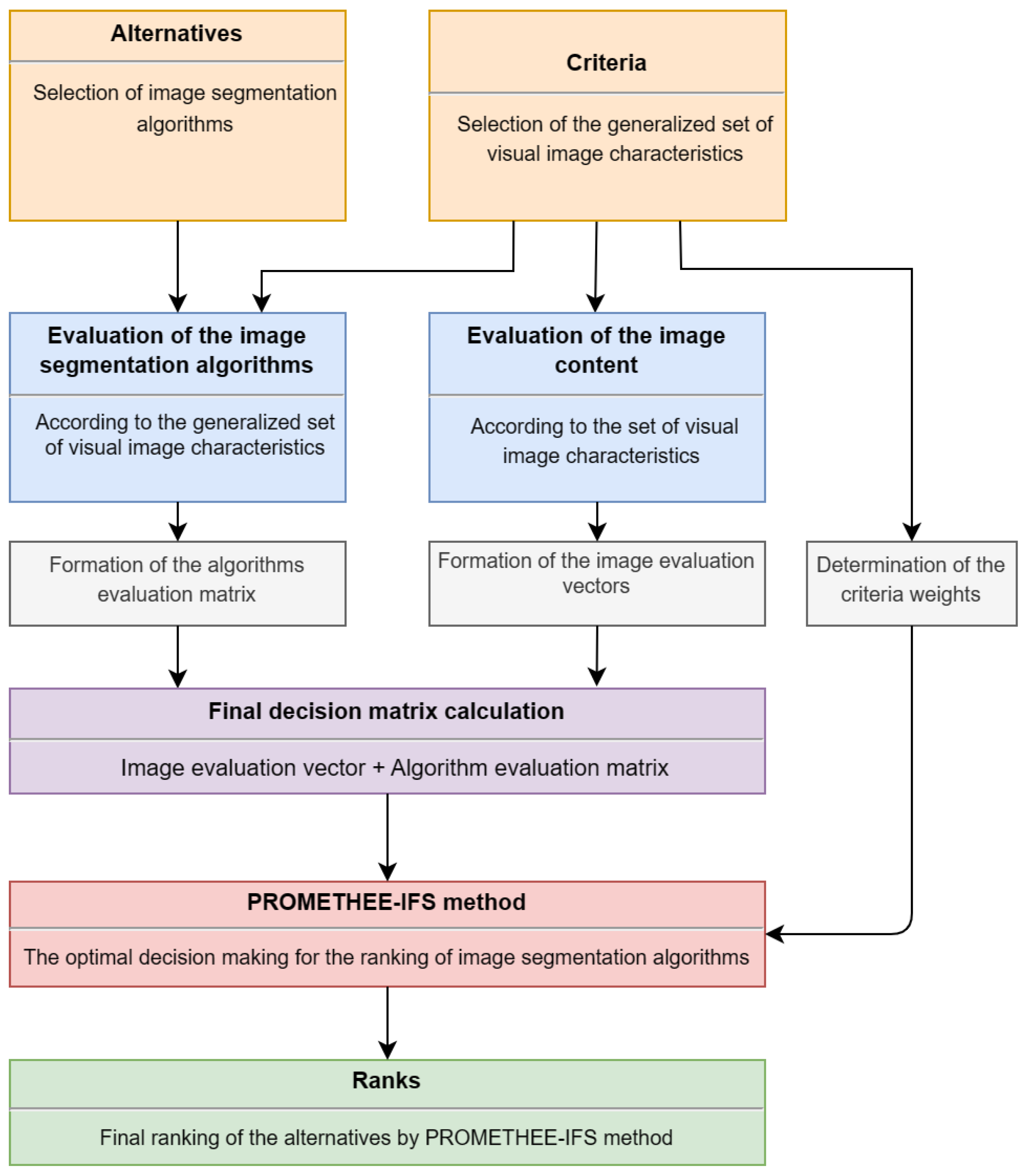
The usual process of evaluating the quality of segmentation involves calculating individual internal, external, or relative metrics without considering several criteria simultaneously. The proposed methodology can be used to determine the most effective segmentation algorithm for specific use cases. The proposed methodology for the selection of image segmentation algorithms includes six essential steps:
Determination of a set of basic visual characteristics (properties) of satellite image content.
Selection of a set of segmentation algorithms.
Evaluation of the influence of the visual properties of satellite images on the result of the respective segmentation algorithms. The images of different content (with the selected visual properties varying within the min–max range) were used to evaluate the algorithms.
Evaluation of satellite image content according to a set of visual characteristics.
Application of the PROMETHEE-IFS method for optimal decision-making using selected criteria weights.
Ranking of segmentation algorithms according to their suitability for the respective type of satellite image.
After obtaining the ranks, additional steps could involve verifying the results, for example, through a subjective quality evaluation.
The suggested approach is represented in
Figure 1. It is versatile and can be applied with any segmentation method, distinct visual image features, or dataset. The method for criteria weights can also be selected according to preference.
3.2. Visual Characteristics (Features) of the Satellite Image Content
Satellite images capture a wide range of visual characteristics that provide valuable information about the Earth’s surface and the objects it contains. Our methodology is designated for selecting the optimal segmentation method considering these characteristics of the image content. Many visual features may significantly influence the results of segmentation algorithms. Thus, in our proposed methodology, the quality of image segmentation is determined by the image content and the sensitivity of the segmentation algorithm, i.e., how certain visual features influence the segmentation result.
For this research, we selected five distinct visual features to construct the initial image vector: contrast, roughness, regions of very small size, distortions of regions, and smoothness (continuity) of region edges. All mentioned visual features are discussed below.
Satellite images with high contrast make distinguishing between different land covers easier, as there is a clear separation between the pixel intensities, improving the segmentation method accuracy for identifying the region boundaries.
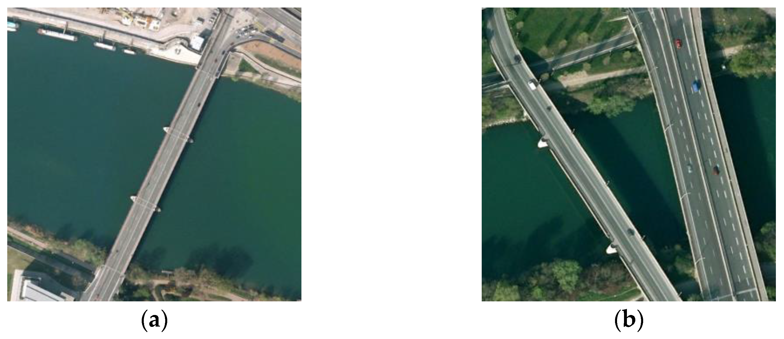
Brightness contrast (or global contrast) determines the difference in brightness between the lightest and darkest parts of an image. An image with high brightness contrast will have bright highlights and dark shadows, while an image with low contrast will have a uniform brightness across the entire image. Color contrast refers to the distinction in brightness between two neighboring colors or overlapping colors, typically involving a foreground and background color [
1]. An image with high color contrast will have vivid and distinct colors, while an image with low color contrast will have muted or similar colors. Color-based image segmentation can sometimes encounter challenges when visually distinct colors are close to each other in the chosen color space and are incorrectly assigned to the same cluster. Contrast adjustment is a common preprocessing step incorporated into various segmentation algorithms to enhance segmentation accuracy by emphasizing edge pixels.
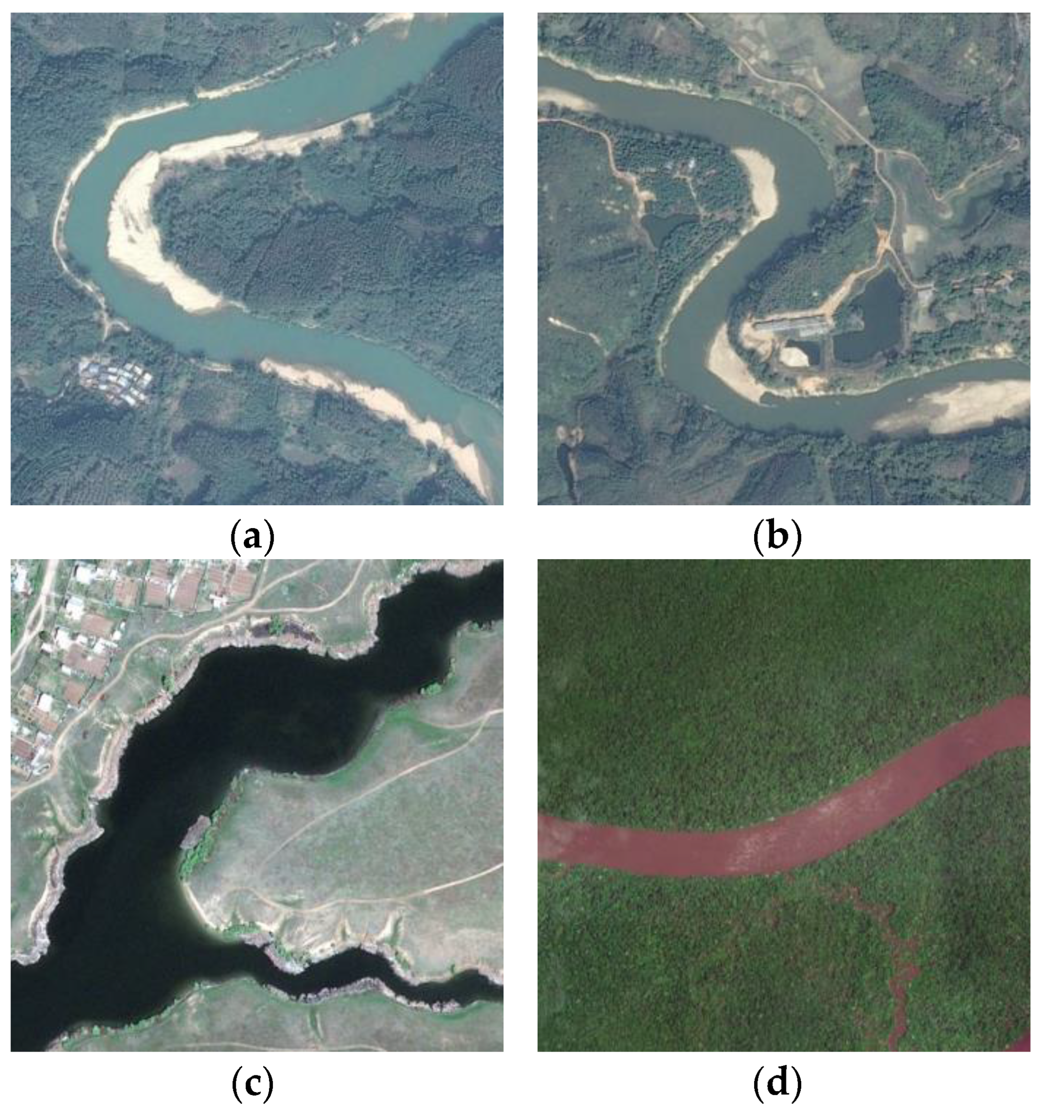
Figure 2 shows low brightness contrast (
Figure 2a,b) compared to high color contrast in images (
Figure 2c,d).
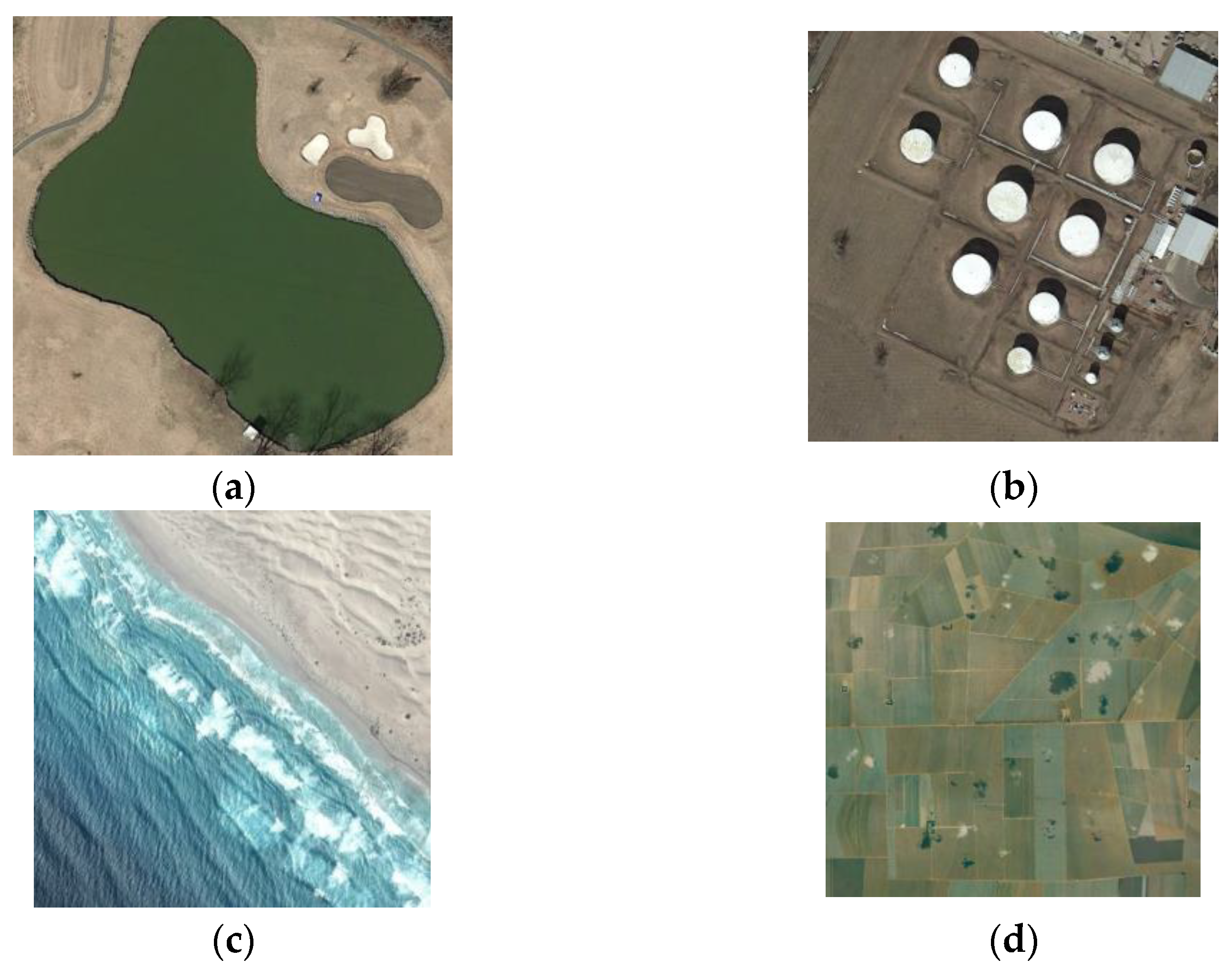
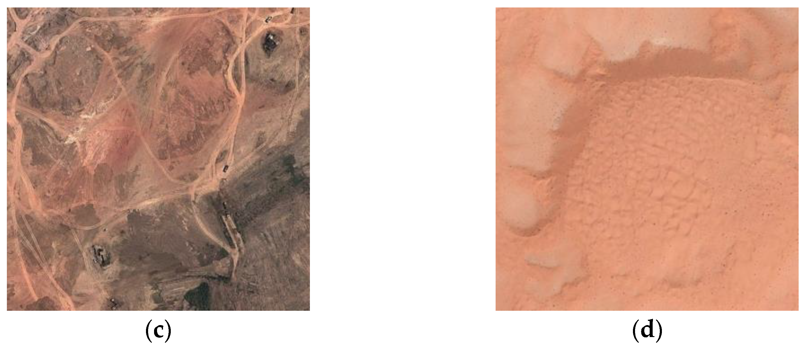
Roughness refers to the degree of irregularity or coarseness in an image’s texture or surface [
22]. This irregularity or coarseness can manifest as pixel color values, intensity levels, or texture pattern fluctuations. In a color image, roughness can be used to describe how color values change spatially. Rapid fluctuations in pixel color values across an area of the image indicate a high roughness (
Figure 3c,d). Low roughness (
Figure 3a,b) suggests a smoother, uniform appearance, such as water, and is easier to segment. While high-roughness regions can be more challenging to segment, roughness can help identify different regions of an image if they have different color fluctuations. Low-level features like roughness may not necessarily correspond to objects with semantic meaning, such as bushes in the desert. High roughness is related to the inherent characteristics of the image or object and represents meaningful visual content. However, high roughness and noise can sometimes be related or occur together. Noise is unrelated to the image and represents unwanted variations introduced during satellite image acquisition or processing.
The characteristics of texture or roughness can vary depending on the direction. Anisotropic texture in one direction (e.g., along the dune crests) might appear relatively smooth and homogeneous. In contrast, in another direction (e.g., perpendicular to the dune crests), the texture might appear rough and exhibit significant changes in pixel values (
Figure 3c).
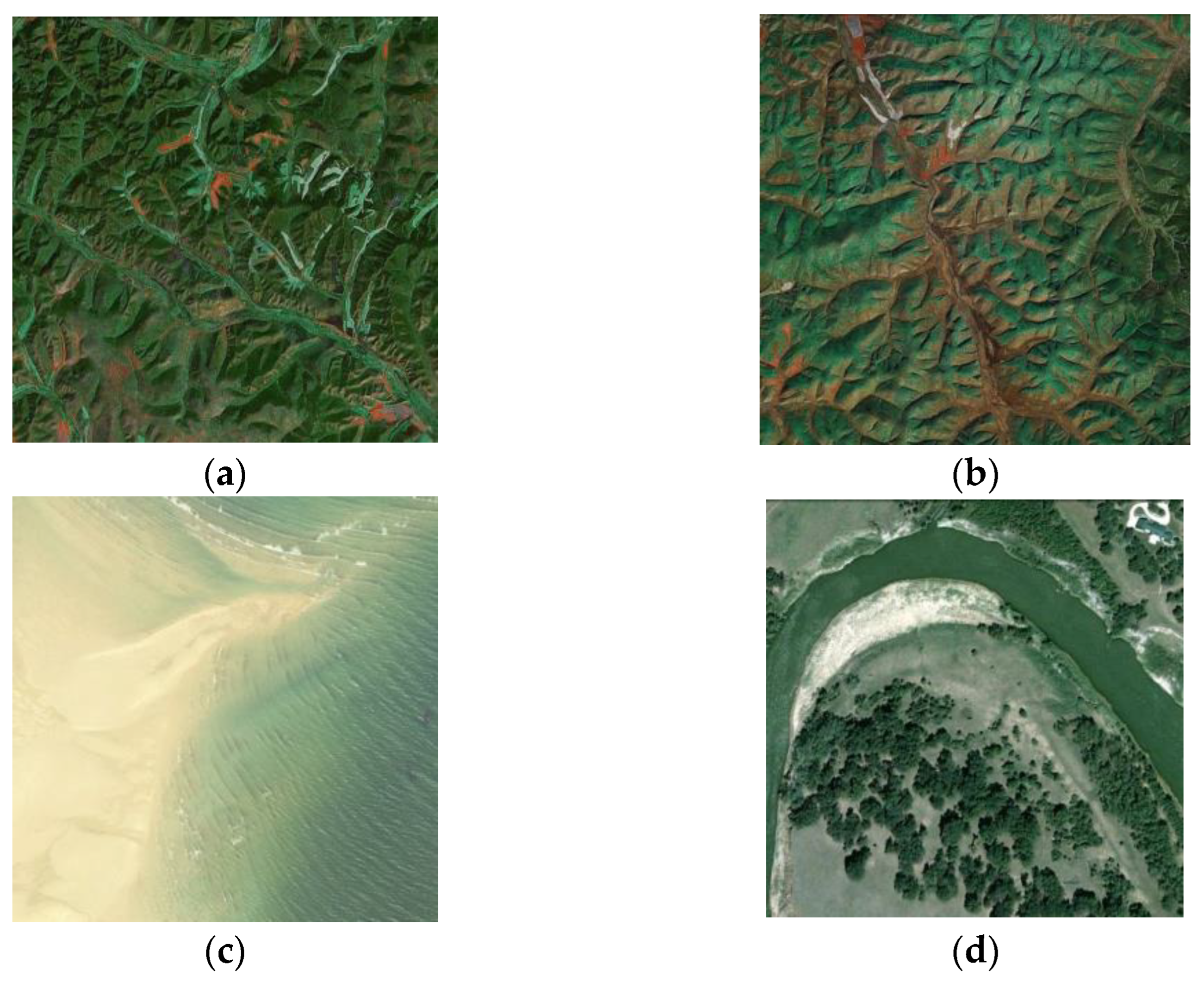
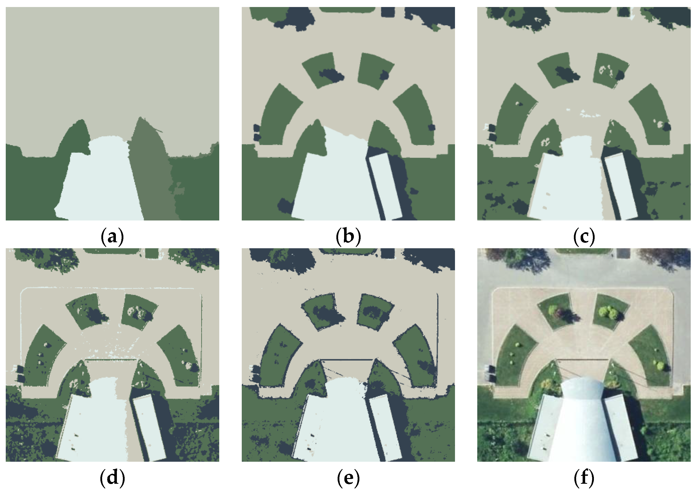
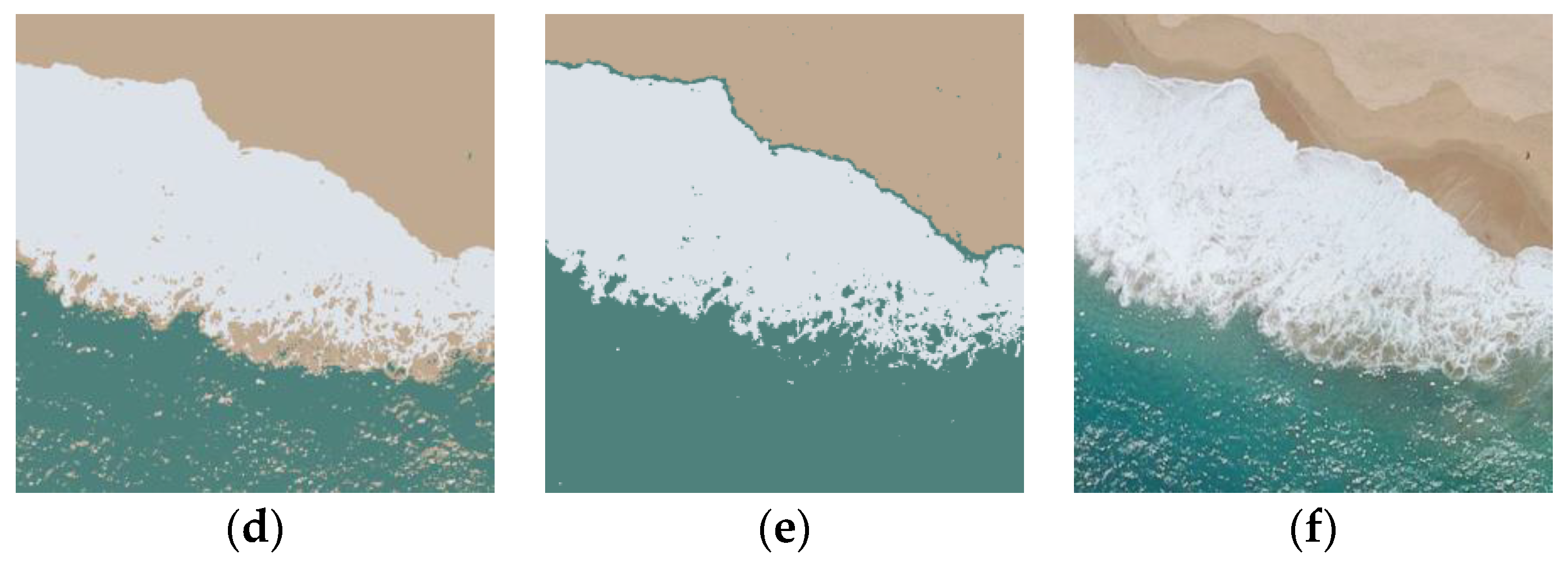
Regions of very small sizes image feature [
34] is related to the number of small clusters in the satellite image. The size of the individual cluster could be determined by the pixel count. In color-based image segmentation, the number of clusters is equivalent to the number of colors perceived by the human eye. Each cluster typically represents a distinct color or a range of similar colors. If the satellite image contains a wide range of distinct color values, the user may set many clusters, with each representing a different color. These clusters have semantic meaning, such as crop fields or buildings (
Figure 4c), and can influence image segmentation in several ways. Generally, the possibility of making errors during segmentation decreases if there are only several big clusters (
Figure 4a) compared to many small clusters (
Figure 4b,d). If the image contains noise or slight variations in pixel values (roughness), these can be misinterpreted as distinct regions when segmenting images with many small regions. This sensitivity to noise can lead to errors in segmentation, resulting in the inclusion of unwanted details (under-segmentation) or the fragmentation of larger meaningful regions (over-segmentation). Many segmentation methods employ region merging and filtering or applying smoothing or noise reduction as the pre-processing step to address these issues.
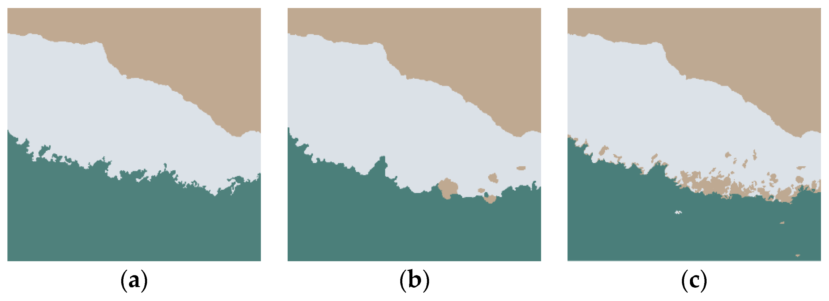
Distortions of regions refer to errors or inaccuracies in delineating and separating objects or regions of interest within an image. These distortions can take various forms, including holes, shadows, clouds (smoke), sea spray (
Figure 5c), or compression artifacts. Shadows (
Figure 5b) in satellite images can be particularly challenging and often mistakenly segmented as part of an object. Changes in lighting conditions can result in variations in the appearance of shadows. Thicker and more opaque clouds can create additional shadows on the ground (
Figure 5d). This can result in overly complex and redundant segmentation results, which may require additional post-processing steps to merge or simplify the segmented regions.
Holes in the segmentation result can be defined as visually noticeable regions in the original image but semantically unwanted within the segmented area based on the context and application. Holes (under-segmentation) can happen due to the presence of low contrast, noise, or the limitations of the segmentation method. If an object in the image is partially occluded by another object or some obstruction, it can lead to holes. For example, the reflection of the tree shadows in the water (
Figure 5a).
Smoothness (or continuity)
of region edges image feature refers to the degree to which the boundaries between different regions in an image are visually coherent and uninterrupted. In the context of image segmentation, the smoothness of region edges significantly affects the accuracy of the segmentation results. If the edges between regions are not smooth enough and exhibit noise or irregularities, it can lead to over-segmentation (
Figure 6a,b). Compression artifacts can break continuous object boundaries into smaller, disconnected segments (jagged edges). This fragmentation can result in the segmentation algorithm treating parts of a single object as separate objects. Jagged edges in satellite or aerial imagery can often be created naturally by tree lines, especially when trees have irregular or densely packed canopies (
Figure 6d). If the edges between regions are overly smooth, meaning they lack sufficient contrast or sharpness (
Figure 6c), it can result in regions being merged or fused, leading to under-segmentation.
Several other features can be considered. If segmentation is based on color, the number of clusters is equivalent to different colors in the segmented image. This feature is influenced by contrast and roughness features. When used as an image segmentation quality metric, the context-dependent nature of such criterion presents challenges that make it less suitable for assessing image segmentation quality. While reducing the number of clusters may be desirable in some cases to simplify an image or emphasize dominant objects, in other cases, maintaining a larger number of clusters can be equally valid, especially when preserving fine details or capturing subtle color variations.
The number of clusters also influences the computational complexity of the segmentation process, increasing processing time. Although comparison and optimization studies [
15,
40] would need execution time as a criterion, time depends on the number of pixels to be processed, the algorithm (or its implementation), and computer specifications. Consequently, this variability can make it more challenging to compare the results obtained by another research directly.
Finally, the shape of clusters can influence the segmentation quality. Different segmentation algorithms have varying sensitivities to cluster shapes. For example, K-means is suited for spherical (convex) clusters, while other methods, such as DBSCAN, are suited for nonconvex clusters [
23]. The shape of clusters feature is again context-dependent, and what might be considered an appropriate cluster shape can differ based on the goals of segmentation or application requirements.
3.3. Segmentation Algorithm Selection
The process of selecting an image segmentation algorithm involves considering various factors and criteria like dataset characteristics and application area. To demonstrate the practical realization of methodology, we selected five soft clustering alternatives: fuzzy C-means (FCM) [
41], superpixel-based fast fuzzy C-means (SFFCM) [
42], significantly fast and robust fuzzy C-means (FRFCM) [
40], robust self-sparse fuzzy clustering (RSSFCA) [
43], and the Gaussian mixture model (GMM). Except for the GMM, all segmentation algorithms are modified versions of the FCM segmentation method. Fuzzy image segmentation algorithms can handle uncertainties and ambiguities in the image data. The original FCM clustering algorithm has been widely applied for image segmentation problems. FCM allows each pixel of an image to belong to multiple clusters simultaneously, which is useful for images with complex textures and overlapping objects. However, FCM has limitations such as sensitivity to noise, initialization dependency, and slow convergence, which led to the development of many modified versions of FCM such as T-spherical fuzzy C-means [
44], improved fuzzy subspace clustering [
45], and an adaptive entropy weighted picture fuzzy clustering algorithm with spatial information (APFCM_S) [
46].
Image segmentation algorithms, including clustering-based methods like FCM, define the objective function that serves as a mathematical representation of the goal the algorithm aims to achieve. The objective function quantifies how well the segmentation algorithm is performing and helps guide the algorithm to find the optimal segmentation solution. The objective function is often designed to be minimized. The classical FCM algorithm defines its objective function as follows:
is FCM’s objective function that aims to minimize the distance between pixels and cluster centers while considering the extent to which each pixel belongs to each cluster. The parameter
m > 1, referred to as the fuzzifier, controls the level of fuzziness in the clustering outcome, with higher
m values resulting in more fuzzy clusters.
C is the number of clusters, and
N is the number of pixels.
is the distance from the
j-th pixel to the
i-th cluster.
is the degree of membership of the
j-th pixel in the
i-th cluster
. Researchers often modify objective functions depending on the image content to enhance segmentation results. A common solution to suppress the influence of noise is the inclusion of (fuzzy) local spatial information inside the objective function [
47].
Traditional fuzzy clustering algorithms encounter several problems. They are sensitive to outliers due to the non-sparse nature of fuzzy memberships. Secondly, these algorithms often lead to excessive image over-segmentation, primarily due to the loss of local spatial information within the image. These issues are solved by the RSSFCA method. The authors define a final objective function in the following form:
represents the distance metric between
and
while also ensuring the requirement of positive values on the distance measure metric. The
denotes the
j-th pixel in the image and
is the
i-th clustering center. Parameter γ is a balancing parameter that controls the sparsity level within memberships. Adjusting the γ value results in variations in the objective function, leading to different levels of resilience to outliers or noise.
FRFCM represents a significant advancement in FCM algorithms, utilizing morphological reconstruction (MR) and membership filtering to enhance speed and robustness. Compared to conventional FCM, FRFCM offers simplicity and significantly improved processing speed, as it eliminates the need to calculate distances between pixels and clustering centers within local spatial neighborhoods. The proposed FRFCM method is executed on the grayscale histogram, resulting in the formulation of the objective function as follows:
represents the fuzzy membership of gray value
l concerning cluster
k;
, and
N is the total number of pixels in the grayscale image
f =
,
is the gray value of the
i-th pixel.
represents the prototype value of the
k-th cluster. ξ is an image reconstructed by MR, and
is a gray level, (1
); q denotes the number of the gray levels contained in ξ. The ξ =
where
is the morphological closing operation and
f is the original image.
The SFFCM method takes a novel approach by integrating the color histogram into its objective function, resulting in a faster segmentation process. The improved performance in color image segmentation is achieved by incorporating both adaptive local spatial information and global color features into the objective function:
l (1
) is the color level;
q is the number of regions of the super-pixel image;
C is the number of clusters;
is the number of pixels in the
l-th region
;
is the color pixel within the
l-th region of the super-pixel image obtained by Multiscale Morphological Gradient Reconstruction-Watershed Transform MMGR-WT [
42].
The GMM involves the superposition of multiple Gaussian distributions. The GMM distinguishes itself by its enhanced ability to handle outliers compared to K-means clustering. However, it does not consider spatial information [
48], which may not effectively process content with noise or complex images. The GMM objective function can be defined as the log-likelihood of the data, which is to be maximized. For an image
consisting of
N data points (pixels) and a GMM with
C Gaussian components, the objective function
can be defined as follows:
where
N is the number of pixels,
C is the number of Gaussian components in the mixture;
is the weight (or mixing coefficient) of the
j-th Gaussian component, with the constraint
;
is the
i-th pixel;
is the mean vector of the
j-th Gaussian component;
is the covariance matrix of the
j-th Gaussian component;
represents the probability density function of a multivariate Gaussian distribution with mean μ and covariance matrix ∑. The GMM’s objective function seeks to find the parameters (
,
,
) that maximize the likelihood of the observed data. This is typically done using the Expectation-Maximization (EM) algorithm [
49], which iteratively estimates the parameters by maximizing the objective function. In the E-step, the algorithm calculates the posterior probabilities of data points belonging to each Gaussian component. In the M-step, it updates the parameters to maximize the likelihood.
The main requirement for the selection of segmentation methods was that the segmentation results created by the selected methods were visually distinguishable and provided different subjective evaluation results. Based on the segmentation tests using the AID, it was noticed that fuzzy subspace clustering (FSC), maximum entropy clustering (MEC), and FCM consistently produced visually very similar segmentation results. Therefore, any of these segmentation methods could have been included in the list of alternatives, but not all together.
Selecting the right combination of parameters for image segmentation algorithms (known as hyperparameter tuning [
23]) is often a necessary starting process. The user is required to provide the number of clusters as input for all segmentation algorithms selected for this case study. The optimal number of clusters is a hyperparameter that needs to be tuned. A common approach for determining the optimal number of clusters is to select the number corresponding to the highest average silhouette score [
50]. However, as this is not the focus of the current research, default segmentation parameters were used, and the number of clusters was set to the dominant colors perceived in the image. Because there were various color shades, we experimented with different numbers of clusters to ensure that the segmentation results matched the human visual system (HVS). No additional pre-processing techniques to improve segmentation accuracy were applied.
3.4. Method for Criteria Weights
Once the set of criteria is determined, the next step is to decide on their relative importance through weighting methods. The evaluation of criteria weights is a common issue that arises in many MCDM methods. Criteria weighting must be carefully selected in most MCDM models because it greatly affects the final ranking of the alternatives [
51]. Weights can be specified by experts (subjective weighting) or calculated via mathematical weighing procedures (objective weighting). In objective weighting, the decision maker has no role in assigning the weights. Using an integrated weighting approach combining subjective and objective weighting methods is also possible. Objective weighting is applied once the data of the decision matrix is known, while subjective weighting can be applied once the criteria set is known. Depending on the characteristics of the decision problem, the available data, and the goals of decision-makers, numerous weighting methods can be used with MCDM.
The stepwise weight assessment ratio analysis method (SWARA) [
52] incorporates individual expert opinions, and it belongs to the subjective weighting method group. Naturally, these methods may require significant time and preparation for participants to evaluate the image content. This can be a drawback, especially when dealing with a large set of subjective criteria, and objective weighting may be more efficient. The entropy weight method (EWM) [
53] is a commonly employed objective weighting method for MCDM problems, which evaluates the degree of value dispersion in decision-making. In contrast to subjective weighting models, the EWM’s primary strength is its ability to eliminate the influence of human factors on indicator weights. However, in certain situations, EWM may also lead to distorted decision-making results.
The SWARA method, which was selected for calculating criteria weights, can be summarized by the following six steps:
- (1)
Identification of the criteria set. This involves defining and selecting the key factors or attributes that are relevant and important to the decision-making problem at hand. The criteria must be clearly defined, measurable, and non-redundant.
- (2)
An expert evaluation is used to sort the criteria in descending order based on their importance. This step provides a starting point for determining the criteria weights. Ten experts consisting of scientists from Vilnius Gediminas Technical University (Vilnius Tech) with teaching experience in image processing were interviewed to rank the criteria.
- (3)
Determining the average value of comparative importance
; how much more important is criteria
than criteria
. The results are presented in
Table 1.
- (4)
The benefits of the comparative importance are calculated as follows:
- (5)
Transitional weights are recalculated, where
j is the index of the criteria:
- (6)
The final weights are normalized, where
n is the number of criteria:
The results are presented in the last column of
Table 2.
Average values of comparative importance
are then used for calculating final criteria weights
by the SWARA method (
Table 2).
3.5. Preliminaries of Intuitionistic Fuzzy Sets
Intuitionistic fuzzy sets (IFSs) extend the concept of classical fuzzy sets by incorporating additional information to deal with uncertainty and hesitation. The main idea behind intuitionistic fuzzy sets is to represent the hesitancy and ambiguity that are often associated with decision-making processes.
First, we discuss the preliminaries of the intuitionistic fuzzy set (IFS) and the algebraic operations (discussed in [
54]) between the intuitionistic fuzzy numbers (IFNs) that are relevant to the proposed PROMETHEE method, namely, PROMETHEE-IFS.
Definition 1. If the domain of problem-related objects is denoted by , is a single object. In this research, is a set of criteria modeled under the intuitionistic fuzzy environment and is a value of a single criterion.
In fuzzy sets, the membership function defines the degree of membership of each element in the set. This function maps each element to a value in the interval [0, 1]. The intuitionistic fuzzy set
consists of two membership functions (fuzzy components):
Here,
is the truth membership function that represents the degree to which an element
x belongs to the set and
is the falsity membership function (or non-membership function) that represents the degree to which an element
x does not belong to the set. Then, the intuitionistic fuzzy set [
14] is defined as follows:
The two membership functions also satisfy the following condition:
The IFS theory also introduces a third dimension known as hesitation function π, which is also called the degree of non-determinacy (or uncertainty) [
14]. This function, of the element
to the intuitionistic fuzzy set
IFS represents the degree of hesitation or uncertainty associated with the element
x’s membership status. This allows for a more realistic representation of uncertainty that may arise during the assessment of segmentation methods.
Here, , . A high value of indicates a higher degree of hesitation or uncertainty regarding whether the element x belongs to the set or not. Conversely, a low value of suggests a more confident or deterministic membership status. This expression ensures that the sum of , , and is always equal to 1. For traditional fuzzy sets, the value of would be equal to 0 for all elements x .
Definition 2. The intuitionistic fuzzy number can be defined as .
Definition 3. Let and be two intuitionistic fuzzy numbers. Then, the summation of the two IFNs can be defined by the following: The multiplication between the two IFNs can be defined by the following:
The multiplication operation between the IFN and a real number
can be defined by the following:
The power function of IFN when
can be defined by the following:
The subtraction between the two IFNs can be defined by the following:
The division between the two IFNs can be defined by the following:
To ensure the stability of the fuzzy set logic, the complementary function of IFN can be defined as follows:
These algebraic operations allow for the manipulation and combination of intuitionistic fuzzy sets to handle uncertainty and hesitancy in various decision-making and modeling scenarios. The choice of specific operations may depend on the problem context, the MCDM method, and the desired behavior of the IFS.
Definition 4. In the defuzzification stage (converting the fuzzy number back to its original crisp form), the score value of IFN can be calculated by the score function proposed by Szmidt and Kacprzyk [55]: If
and
are two intuitionistic fuzzy numbers, the comparison of them is determined by score values:
3.6. PROMETHEE-IFS Method
A new extension of the PROMETHEE method under the intuitionistic fuzzy set environment, namely PROMETHEE-IFS, is designed and presented in this section to solve the selection of the image segmentation algorithm for satellite images. The main steps of this approach can be expressed as follows:
- (1)
The solution procedure of the PROMETHEE method starts with the constructed initial algorithm evaluation matrix
which consists of the elements
and is defined as follows:
The element
represents the assessment of the
i-th alternative (algorithm) by the
j-th criterion (image features). For this test case, additional information is included by evaluating the image content based on the same criteria. These expert evaluations can also be expressed in linguistic terms (
Table 3) and are used to create an image vector
that has the same number of elements as the columns in the algorithm evaluation matrix
.
- (2)
Vector normalization is applied to the algorithm evaluation matrix
elements
to obtain a normalized algorithm evaluation matrix
:
Additionally, a normalized image assessment vector is calculated.
- (3)
Fuzzification is a fundamental process in fuzzy logic that involves converting crisp or precise data, which typically consists of numerical values, into fuzzy data. Fuzzification of the normalized decision matrix
is performed by mapping crisp values (expert evaluations) to fuzzy values, as displayed in
Table 3. In this step, every member
of
is replaced with the intuitionistic fuzzy numbers
as in
Definition 2. Intermediate values are obtained via linear interpolation. As a result, the intuitionistic fuzzy decision matrix
is created. Similarly, we perform the fuzzification of the normalized image assessment vector
to obtain an intuitionistic fuzzy image assessment vector
.
A special step is proposed and performed to obtain the final decision matrix
by fuzzy column-wise addition (Equation (13)) of the fuzzy image assessment vector
and the fuzzy algorithm evaluation matrix
:
This integration improves the selection process of the appropriate segmentation algorithm by considering both the visual image characteristics and the algorithm’s sensitivity to these characteristics. These evaluations for the algorithm matrix are left constant throughout the experiment, while the image content vector varies for each satellite image. The final decision matrix is then formed from these two elements by fuzzy fusion. In this way, the decision matrices are computed for all test images.
- (4)
To rank the alternatives using the PROMETHEE-IFS method, a comparison is made between each pair of alternatives (
and
) by calculating the aggregated preference function
using the following equation:
Here, are weights (of the i-th criterion) obtained from the SWARA method . If , the difference between two IFNs is calculated as , and if , the difference is calculated as . (Equation (17)).
corresponds to the value of the i-th criterion of the alternative , and corresponds to the value of k-th criterion of the alternative .
is the
k-th preference function (
Figure 7) for the
i-th criterion selected from the six types of criteria functions proposed by the authors of the PROMETHEE method.
The preference function assigns values between 0 and 1 to quantify the degree of preference or indifference between two alternatives. Here, p and q are the preference function’s thresholds, i.e., the maximum and minimum values of the selected criteria.
- (5)
Calculation of the positive outranking flow:
Calculation of the negative outranking flow:
- (6)
Calculation of the positive net flow value
is a step that needs to be performed to determine the final rank of the alternative
. This value is obtained by subtracting the negative flow values from the positive flow values:
Note: To accommodate the characteristics of fuzzy sets, such as the non-negativity of fuzzy numbers, the calculation of negative net flow values is carried out using additional intuitionistic algebra, which can be represented as follows:
- (7)
Defuzzification is the reverse process of fuzzification, where fuzzy data is converted into crisp data. The process of defuzzification of the net flow value involves calculating the score function for each alternative . Based on values, the ranking of the alternatives is determined as described in Definition 4.
The sign of the final results of PROMETHEE-IFS is interpreted by directly ranking the alternatives with a positive score value , where the best alternative would have the highest score value. However, for negative score values, the best alternative is the one with the smallest score value.
4. Application of Methodology for Satellite Images
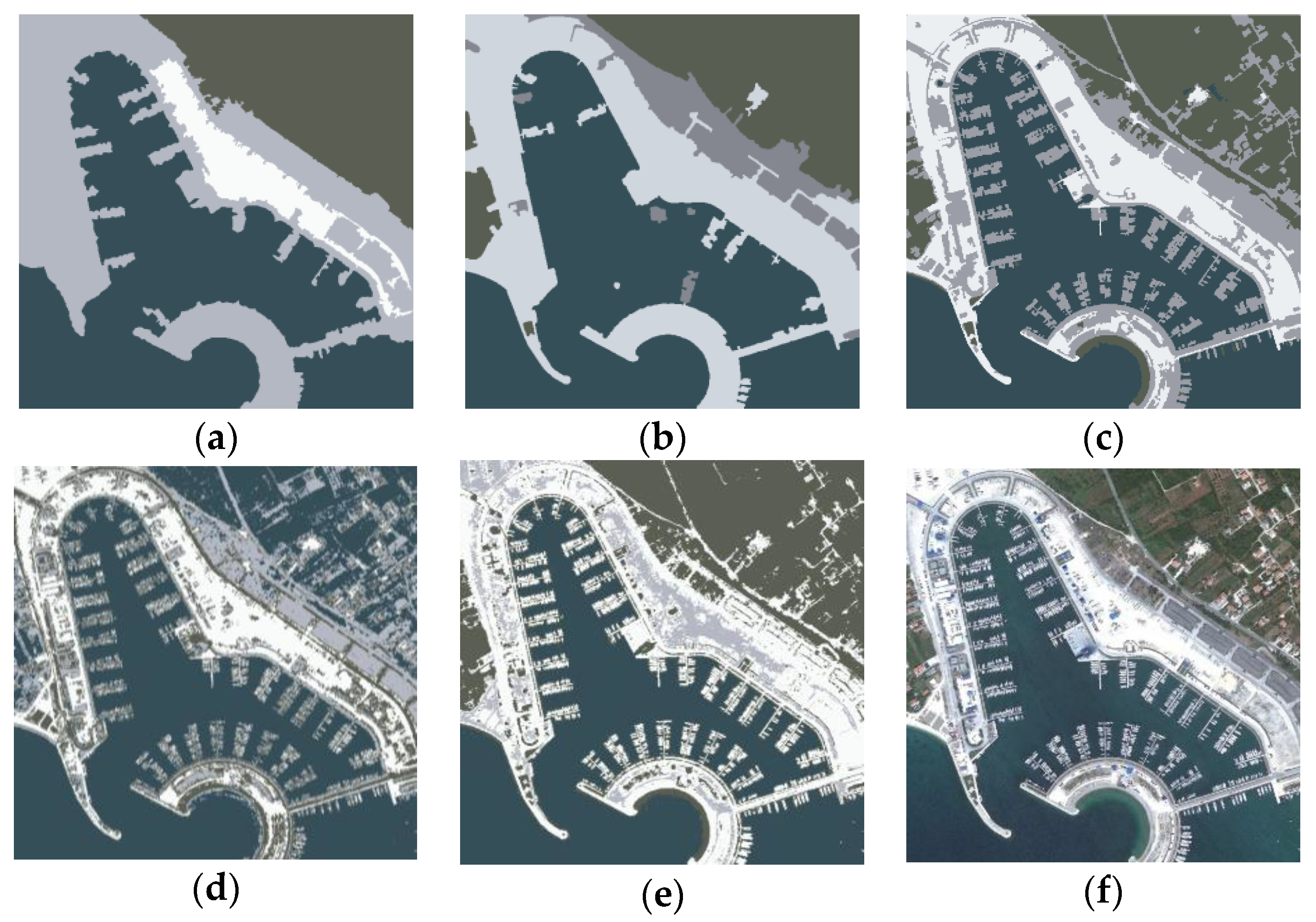
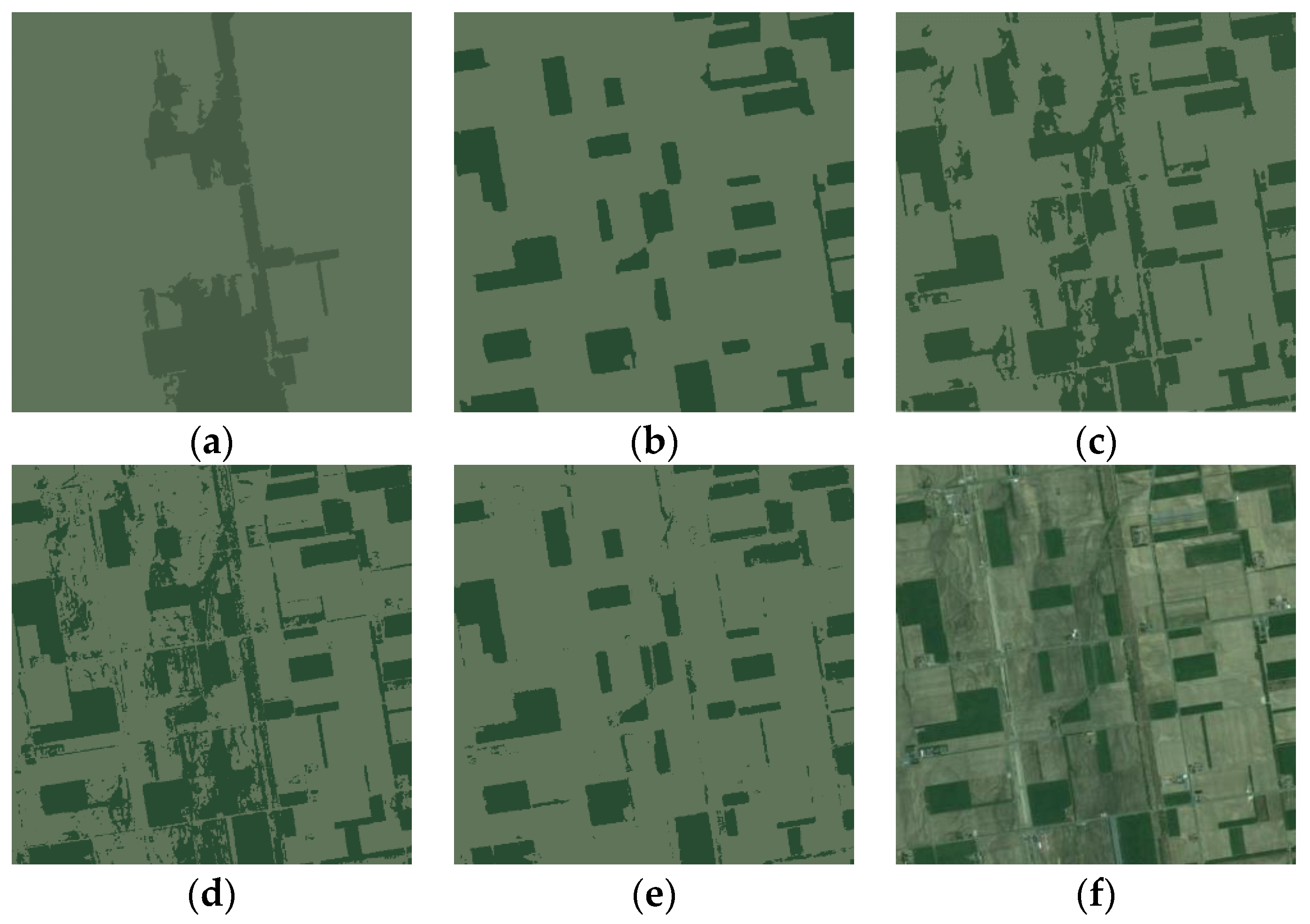
This section briefly discusses the dataset and the initial decision-making matrix creation. It displays the final ranking of segmentation algorithms produced by PROMETHEE-IFS that demonstrates the optimal method for each test image. Finally, the verification step is performed by comparing the average expert rank with the average rank by the PROMETHEE-IFS method. In addition, a rank sensitivity test has been conducted.
4.1. Selection of the Dataset
After analyzing the visual characteristics of the satellite image content most important for segmentation, selecting an appropriate dataset becomes the next crucial step.
Usually, a large sample of images can enhance the precision while evaluating various machine-learning methods. However, a large dataset is not needed for our proposed methodology. The goal is to select the test images with the most prominent visual features (described in
Section 3.2).
The Aerial Image Dataset (AID) [
39] is a large-scale aerial scene classification dataset that was selected for this experiment. The AID dataset is larger than the popular UC Merced Land Use dataset. It contains 220–420 images per class (10,000 images in total) in RGB color space, a size of 600 × 600 px, 24-bit JPG image format with a multi-pixel resolution that varies from approximately eight meters to half a meter. Files are named using the following format: <CLASSNAME_ID>.jpg, where ID is a numeric value that varies depending on the class of aerial scene.
AID is divided into 30 classes: (1) airport, (2) bare land, (3) baseball field, (4) beach, (5) bridge, (6) center, (7) church, (8) commercial, (9) dense residential, (10) desert, (11) farmland, (12) forest, (13) industrial, (14) meadow, (15) medium residential, (16) mountain, (17) park, (18) parking, (19) playground, (20) pond, (21) port, (22) railway station, (23) resort, (24) river, (25) school, (26) sparse residential, (27) square, (28) stadium, (29) storage tanks, and (30) viaduct.
All of the images were acquired at multiple locations, varying times and seasons, and under diverse imaging conditions, resulting in increased intra-class diversity within the data [
39]. An image pair (a, b) in
Figure 8 provides an example of the same class/object but at a different scale and lighting conditions. The smaller inter-class dissimilarity feature of the dataset is illustrated by image pair (c, d). Rough or uneven textures composed of grain and similar colors characterize both bare land and desert classes. The only difference is that the bare land class typically contains clear roads and smaller solitary objects such as buildings.
The higher complexity of the dataset provides more meaningful results for investigating the sensitivity of the segmentation algorithms to visual features of images. More complex content can better highlight the shortcomings and advantages of different methods since most methods will usually perform well with simple image content or a low number of clusters [
42].
4.2. Subjective Image and Segmentation Method Assessment
In order to apply the PROMETHEE-IFS method for selecting the best-performing segmentation algorithm for a specific image, developing an initial decision-making matrix is required. This section describes the subjective assessment used to construct the initial decision-making matrix. The subjective assessment consists of two parts:
- (1)
Evaluation of the sensitivity of the segmentation method according to individual visual image characteristics to obtain segmentation algorithm evaluation matrix
In the initial experiment, five image segmentation algorithms were evaluated: FCM, SFFCM, FRFCM, RSSFCA, and the GMM. The content of the selected images influences the segmentation results. The sensitivity of the algorithms to the image content was evaluated by presenting the segmentation results to the group of ten experts. The experts were asked to assess how each algorithm processes satellite images with specific visual content. The sensitivity measurement was based on a (1–9) rating scale. The mean values of these assessments were calculated as presented in
Table 4. The same group of experts provided their opinion on the weights of the visual criteria described in
Section 3.4.
- (2)
Evaluation of the presence of visual features in the image content to obtain an image assessment vector
. The second part of the evaluation was aimed at assessing the content of the images by analyzing their visual features. A set of proposed visual features that characterize satellite images was constructed (in
Section 3.2). We have selected images that best represent each visual feature for this test case. Before the image content evaluation process, a group of ten experts was given visual criteria (characteristics) definitions, a rating scale, and information on what is considered to be a minimum and a maximum value of each criterion. A (1–9) rating scale was used to evaluate the image content, and the mean values of the content assessments were subsequently calculated (
Table 5).
Evaluation results of algorithm sensitivity are presented in
Table 4, and the assessment of image content is shown in
Table 5.
denotes the alternative (segmentation method), and
denotes the criteria.
The optima in
Table 4 and
Table 5 refer to the optimization direction of the selected criteria. There are two possible optimization directions—
max and
min. The
max optimization direction aims to maximize the performance associated with the (
) criteria. In such cases, the optimization direction of the criteria is towards higher values, and better alternatives will achieve higher possible performance on the criteria. The
min optimization direction aims to minimize the negative impact associated with the
criteria. In such cases, the optimization direction of the criteria is towards lower values, and better alternatives will achieve lower possible performance on the criteria.
The elements of the final decision-making matrix are then calculated by fuzzy addition operation (Equation (13)) by adding an image column vector in
Table 5 to each of the segmentation algorithm’s columns in
Table 4. The resulting matrix
contains the criteria
in the rows and the alternatives
in the columns and is used for decision-making.
4.3. Ranking of Segmentation Algorithms
The FCM and the GMM effectively preserved more details and provided relatively precise boundaries between clusters. However, improved RSSFCA and SFFCM methods returned smoother clusters with reduced noise and artifacts. At the same time, FCM and GMM methods are more sensitive to lossy compression artifacts if present in the image. The FRFCM method was a balanced solution between FCM and the GMM (which overly replicates the original image) and SFFCM and RSSFCA algorithms (clean clusters, but excessive merging).
From the overall results in
Table 6, the classical segmentation method FCM obtained one first place and the GMM two first places. Similarly, SFFCM obtained one first place and FRFCM two first places. Other special situations are presented in the discussion section. Thus, we can note that the quality of the results of segmentation algorithms depends on the image content’s characteristics and the algorithm’s sensitivity to the corresponding visual characteristics of the image.
4.4. Verification of Methodology
Alternative methods were used to validate experiment results to confirm the dependability of the ranking results of PROMETHEE-IFS. PROMETHEE rankings of each of the six test images are compared to the expert rankings.
The experts evaluated the visual quality of each segmentation and ranked segmentation methods from 1 (best) to 5 (worst) in
Table 7. The original image was provided for reference. For example, expert 1 rankings for square_1 are 4, 3, 1, 2, and 5; expert 2 rankings for square_1 are 1, 4, 3, 2, and 5, etc. Since the ranks are restricted to a small range of values and rank scores do not contain outliers, the arithmetic mean was used for the average score/rating of all expert evaluations. The average rank value by the PROMETHEE-IFS method is then compared to the average expert rank value in
Table 8.
The ranks created by PROMETHEE-IFS and experts can be categorized as ordinal data, so the rank difference sign in
Table 8 does not necessarily have a meaningful interpretation in this context.
The average expert rank can be calculated in several ways. First, calculate the average value for each image and then find the final average between these averages. In addition to the final average, this approach allows the assessment of individual averages for each image individually. The final average (FA) score can be expressed as follows:
where
is the total number of experts,
represents the evaluation of the
j-th image by
i-th expert, and
is the number of images in the set.
The percentage difference in
Table 8 represents the relative difference between the two values and can help assess the magnitude of the difference meaningfully. When calculating the percentage difference, the average of the two scores was used in the denominator for relative comparison:
Here,
A is the expert rank and
B is the PROMETHEE-IFS rank from
Table 8. We aim for the ratings obtained using the PROMETHEE-IFS method to be as close as possible to experts, as expert ratings are selected for validation.
In
Table 8, the experts’ ranking differs from PROMETHEE-IFS because it is challenging to decide which ones to prioritize when a person evaluates a segmented result against a set of features. The MCDM method helps to overcome this problem and evaluate the result according to individual criteria by combining them to calculate the ranking.
Comparing MCDM methods can be challenging because their performance often depends on the alternatives used (in our case, algorithms), the set of criteria, the application area, and the problem being solved. An additional experiment was conducted to assess the sensitivity of image content evaluation and validate the proposed methodology. Sensitivity analysis [
56] is an important step in the assessment of the reliability of MCDM methods. This analysis relies on the precision of image assessments, specifically, how the oscillations of the respondents’ evaluations affect the selection of segmentation algorithms.
Two new groups, consisting of students and experienced users, evaluated the image content according to the given criteria. The image “square_1” was taken for sensitivity analysis. After the content was evaluated, two new sets of rankings were compared. The impact of rank sensitivity analysis is presented in
Table 9, and its visualization is shown in
Figure 15. A robust method should handle small variations in ranking data without significantly altering the overall decision outcome.
The assessments presented in
Figure 15 lead to the conclusion that for the square_1 image, both the experts and experienced users regarded the FCM algorithm (preserved more details) as the best choice, while students preferred the FRFCM algorithm (less noise).
5. Discussion
The goal of this research is to propose a methodology by extending the PROMETHEE MCDM method through IFS and applying it to the selection of optimal segmentation methods for satellite images. The selection of the optimal algorithm depends on the subjective visual characteristics of the satellite images being analyzed. Different segmentation methods may excel in different scenarios based on the desired outcome, application, or characteristics of the data set [
57]. In the segmentation of satellite images, the objective is often to accurately identify and separate various regions by specific criteria, as described in
Section 3.2. These five criteria related to satellite image content were selected and used for content evaluation. The segmentation algorithms were evaluated according to the same criteria.
Table 8 shows a correlation between subjective (expert ranks) and objective ranks produced by PROMETHEE-IFS. In all cases, the rank difference is less than one rank. The visual ranking of segmentation results revolved around balancing under-segmentation and over-segmentation.
The results in
Table 2 indicate that
(contrast) is the most important criterion, while
(smoothness) is the least important criterion in the list. This outcome can be attributed to the fact that human visual perception can tolerate certain types of distortions while being very sensitive to others. For example, humans can tolerate border holes to some extent, which is known as human visual tolerance [
27]. This could explain the difference in obtained SWARA weightings for
and
criteria.
The test results in
Table 6 show that even classic segmentation methods (GMM and FCM) may achieve better results than modernized versions depending on the content. In addition, some segmentation algorithms may be tuned against over-segmentation, so images with small objects may not have a clear separation (under-segmentation). For example, the RSSFCA is tuned against over-segmentation and obtained the worst expert and PROMETHEE-IFS ranks, as it often unnecessarily merged regions, such as dunes in desert_23 or did not preserve finer details (smaller lakes in river_237). On the other hand, RSSFCA yielded better results in the case of the beach_19 image dominated by three large clusters, suggesting its suitability for less complex content.
Compared to another classical method like the GMM, the FCM fails to correctly separate between blue coastal water and green fields in port_19, which is possibly due to several contributing factors. In a given dataset, the GMM treats the input data points as being generated from a mixture of several Gaussian distributions. This modeling approach is often more suitable for capturing the distribution of colors and their variations. Overall, the GMM outperformed FCM (
Table 8) due to being more robust to noise than FCM. The GMM can provide a more flexible representation of the data density in the feature space. This can be especially beneficial when dealing with regions with smooth color transitions. Moreover, light green and cyan are relatively close to each other in the RGB color space, so an algorithm like FCM that relies on the default Euclidean distance in the RGB color space might fail to distinguish between shallow water and grass.
Small expert and PROMETHEE-IFS rank differences, such as for SFFCM, can be interpreted as a stable segmentation solution in relation to other methods. In this case, the SFFCM method produced consistent results (2–3 places) in all segmentation scenarios.
Conducting a comprehensive comparison with existing research results is challenging. However, we can refer to the articles in which our selected algorithms are evaluated. For example, the rankings provided by PROMETHEE-IFS align with the findings presented by the FRFCM authors [
40], particularly in scenarios involving noise (see
Table 3 and
Table 4 from the original article). Our proposed method also selects FRFCM over FCM in the cases of more noisy desert_23 and river_237 images. The FRFCM method achieved the best expert and PROMETHEE-IFS ranks (
Table 8) since morphological reconstruction (MR) effectively suppressed noise while maintaining precise object contours.
The result validation in
Table 8 showed that the proposed PROMETHEE-IFS correlates with a subjective evaluation with an accuracy of less than one rank, confirming the effectiveness of the proposed method. At the same time, the rank sensitivity analysis in
Table 9 shows rank differences between alternatives within one rank, validating the robustness of the methodology. For example, despite minor differences in evaluations across all evaluator groups, the RSSFCA method consistently ranked last due to its visually worst segmentation results.
Subjective evaluation methods can be adapted to different types of content. They can be used to evaluate different aspects of image content or quality, such as image sharpness, color fidelity, or contrast. In the context of our research, this adaptability could be particularly valuable when describing the feature-rich content of satellite images.
The user is mostly interested in a situation where the image segmentation methods return visually distinct results (i.e., the clear winner is not apparent). In such cases, human judgment can provide insight into the quality and appropriateness of the segmentation result that objective metrics may not always capture. In cases where the segmentation method always gives a poor result (especially with complex images), there is no need to use our methodology since such a method will always be in the last place. Alternatively, if all segmentation methods return visually similar outcomes (especially with less complex images), there is no necessity to determine the optimal method.
Subjective content evaluation methods can provide insights into the overall perceptual aspects of the image content. While most visual image features may be relatively independent of others, there is typically some level of interdependence. Combining objective and subjective evaluation criteria can achieve a more comprehensive evaluation of image content. However, our task is to combine the features of the image content with the evaluation of algorithms, which was achieved during step 3 of the proposed PROMETHEE-IFS method.
6. Conclusions and Future Work
Image segmentation algorithms may not always return accurate results due to the image complexity and different image content. Therefore, identifying the most appropriate method for the specific image content is often essential. This paper proposed an approach that extends the PROMETHEE method via intuitionistic fuzzy sets and combines it with the SWARA weighting model for selecting optimal segmentation methods for satellite images. This study used five subjective visual features: contrast, roughness, regions of very small size, distortions of regions, and smoothness of region edges. A novel way of forming a decision matrix was used by combining information from two different sources (image assessment vector and the fuzzy algorithm evaluation matrix). Average rank comparison and sensitivity analysis confirm that the proposed PROMETHEE-IFS method is well-suited for the selection of segmentation algorithms for satellite images.
Image content characteristics are often interrelated. Changing one image feature leads to changes in other image features (increased contrast can create more separation between adjacent colors). Different segmentation algorithms have varying sensitivity and interpretation of image content features. Thus, no one algorithm fits all content. Both the results of this experiment and the verification confirm the NFL theorem [
58] in the context of image segmentation. This again underlines the importance of considering the characteristics of the images when choosing or developing segmentation algorithms.
This methodology can be used with other subjective visual features; however, the features must have a clearly defined optimization direction, i.e., minimum and maximum values. If a feature does not have a logical minimum or maximum value that could affect the quality of segmentation, such a criterion cannot be easily included in the initial decision matrix. For example, mathematically quantifying the shape of clusters (as a visual feature) in a way that applies universally across diverse image content and domains might be challenging.
A single image may not fully represent specific features or the class it belongs to. This is especially true for general-purpose image datasets that lack specific categorization or are not created for a particular task or application. Applying the suggested method to a larger set of images might be necessary in such a case.
The following further research perspectives may be included:
In general, MCDM methods can be applied to optimize the segmentation algorithm, particularly fuzzy logic-based segmentation methods [
60]. By incorporating MCDM methods, these algorithms can be further optimized to provide more accurate segmentation results. Finally, the proposed approach can be adapted to select the optimal number of clusters problem, where within a given dataset, different numbers of clusters would be represented as potential alternatives.


