Computational Assessment of the Deposited Power and the Temperature Increase around Two Coupled Implanted Leads Inside a 1.5 T MRI Scanner

Featured Application

Although, during an MRI scan based on ISO/TS 10974:2018, an assessment of the enhanced tissue heating due to coupling between leads of close proximity should be performed, a specific method for this estimation has not been defined. Therefore, the aim of this work is to evaluate a numerical method, similar to the Tier 3 process, for the estimation of the deposited power at the tips of two coupled implanted leads with a 1.5 T coil. Furthermore, in a previous work, an experimental process was proposed on a parallel couple of cables with a constant distance between them; our method advances this model, allowing the calculation of the deposited power for realistic in vivo implant placements and not only for the parallel placement of leads. Our proposed method is totally numerical, as the experimental measurement of the temperature increase at the in vivo placements of implants could not be feasible.

Abstract

A specific method for the estimation of the induced power at the tip by an active implantable medical device (AIMD) during an MRI scan is not defined in ISO/TS 10974:2018 for the cases of devices with multiple leads or the presence of abandoned and retained leads, where coupling between two leads could take place. Therefore, the aim of this work is to evaluate a numerical method, similar to Tier 3 of ISO/TS 10974:2018, for the estimation of the deposited power at the tips of two coupled implanted leads. Specifically, the proposed methodology applies the same parameters as the standard Tier 3 process. However, these parameters are calculated for each implant in the presence of its neighbors in order to include the coupling between them. Numerical electromagnetic simulations were performed, in which a pair of generic implant leads was excited and placed at various positions relative to each other. The deposited power at the tips of the pair was analyzed based on the standard Tier 3 approach, and the results show that this could overestimate the induced power by more than 6 dB. Therefore, a modified Tier 3 numerical method for the estimation of the deposited power at their tips is proposed, which can produce a reliable calculation. This method was confirmed by evaluating various configurations of the two leads excited by orthogonal electrical fields, and also its uncertainty budget was developed. Finally, the method was repeated for different properties of the generic implants and the surrounding tissue, as well as for a pair of realistic implants and in vivo implantation trajectories.

1. Introduction

Magnetic resonance imaging (MRI) is an important technique in medical diagnostics with continuously increasing applications. Nevertheless, many patients with active implanted medical devices (AIMDs) in their bodies are excluded from this procedure. The reason for this exclusion is the interaction of AIMDs with the radiofrequency (RF) fields of the MRI scanner, leading to unwanted and potentially dangerous tissue heating at the tip of leads [1]. However, the growing number of implanted medical devices and MRI scans led to the necessity of assessing the MRI safety of AIMDs [2,3,4]. Several previous studies have presented in vitro measurements of the induced heating at the tip of an implanted lead, as well as in vivo measurements for specific electrodes, MR systems and conditions [5,6,7,8,9,10].

In addition, previous works have studied several factors that influence the amount of heating at the lead tip, such as lead geometry, conductivity of the medium at the lead tip, location of the implant inside the body, position of the phantom inside the coil and the MR system used [11,12,13,14,15,16,17]. In order to calculate the temperature rise in tissue caused by an AIMD during an MRI session, a technical specification has been developed by the International Organization for Standardization (ISO) [18]. This specification contains a four-tier approach with increasing complexity and accuracy of estimation between successive tiers. The lower tiers are based on simplifications of the exposure situation, producing an overestimation of the temperature increase and, therefore, resulting in a larger safety margin. On the contrary, the higher tiers involve the realistic implant placement of AIMDs in the human body and the accurate calculation of the incident fields, reducing the overestimation and resulting in a more realistic evaluation of the temperature rise. In particular, the Tier 3 approach uses the concept of the transfer function (TF) of an implant and correlates the incident tangential electric field along a trajectory to the deposited power in the tissue surrounding the lead tip, which leads to the temperature increase [19].

The above-described process refers to a single lead. However, many implants, such as conventional pacemakers, deep brain stimulators, spinal fusion and nerve cuff stimulators, have multiple leads resulting in a mutual coupling between their currents induced by the RF field inside an MRI scanner [20,21,22,23,24]. Aside from these multiple-lead implants, there are cases, where, due to a technical failure, an implant should be extracted and replaced by a new device. The incomplete lead extraction could result in abandoned or retained leads inside the patient running in proximity to newly implanted leads [25,26].

A dedicated approach to assess the potential coupling impact arising from devices with multiple leads or the presence of multiple leads, such as those found in instances of either abandoned or retained implants, has not been established to date. However, the presence of a second wire changes the TF of the single wire, causing either an increase or decrease in the current amplitude along the wire [27]. Moreover, ref. [28] concluded that the presence of an abandoned lead modified the heating profile of an MR-conditional implant, resulting either in an increase or a decrease in the induced heating, depending on the relative position of the two leads. Similarly, previous studies showed that the presence of abandoned or retained leads could pose an additional risk to the patient [25,26]. In [29], it was reported that a broken lead enhanced the deposited power at the tip compared to the intact lead, whereas the proximity of an intact wire or even a nearby broken wire reduced the enhancement factor. In another study, the mutual coupling of the wires was used to minimize the RF heating through the addition of one or more coupled fillers to the lead [30]. In [31], the strong influence of the coupling between leads on the resulting heating was demonstrated, and the authors proposed an additive transfer function model to evaluate the heating of the coupled leads.

Thus, there is a need for a Tier-3-like process for multiple functional leads and their abandoned or retained counterparts located at various relative positions between them; this is the aim of the current work. We propose a numerical method to estimate the deposited power at the tips of device leads implanted next to each other, based on the TF approach. In order to show the various steps of the new evaluation, we chose to apply it to a pair of generic leads, in the form of uncapped wires, without the loss of generality in the case of leads of commercial implants. Moreover, we developed the uncertainty budget of the introduced numerical method and we performed numerical calculations for realistic implants and trajectories inside a homogenous human model.

2. Materials and Methods

2.1. Transfer Function of a Single Lead

According to the Transfer Function approach, the power deposition at the tip of the implanted lead is determined by

$$\mathrm{P}=\mathrm{A}{\left({\int }_{\mathrm{L}}^{}{\mathrm{E}}_{\mathrm{t}\mathrm{a}\mathrm{n}}\left(\mathrm{z}\right)\mathrm{S}\left(\mathrm{z}\right)\mathrm{d}\mathrm{z}\right)}^2,$$

(1)

where S(z) is the transfer function (TF), A is a calibration factor and E_tan (z) is the tangential component of the incident electric field along the lead path L inside the patient, without the lead in place [19]. Thus, the TF decouples the scattered field from the incident field and is usually assessed experimentally, using a piecewise excitation method. In the latter, a localized electric field is applied along the implant and the TF is obtained by measurements of the resultant electric field at the tip of the implant. Alternatively, the TF can be evaluated using the theorem of reciprocity by exciting the tip of the implant and monitoring the induced current distribution that directly reflects the TF [32]. The latter approach provides the advantage of requiring only two simulations for the numerical determination of the TF [33].

In this work, the reciprocity approach was employed to determine the electrical model of a generic lead, 40 cm long, at 64 MHz. In particular, the implanted lead was modeled as a straight wire of 1.6 mm diameter, isolated by a tube of 0.9 mm thickness with ε_r = 3, and with 1 cm of insulation removed at both ends (uncapped wire) [19]. The TF was numerically assessed with full-wave simulations using Sim4Life V6.0 (SPEAG, Zurich, Switzerland), where the lead was placed along the z-axis in an infinite in all dimensions, lossy, high-permittivity, tissue-simulating material (HPM, ε_r = 78, σ = 0.47 S/m). The lead was excited by a 1 A current source at the tip and the grid of the simulations was set to 0.1 mm × 0.1 mm × 0.3 mm. The calibration factor A was estimated using a plane wave excitation of 1 V m⁻¹ rms at the lead and matching the absorbed power numerically calculated at the lead tip through the computer simulation with the absorbed power assessed by the TF and the incident tangential electric field along the implant trajectory. The numerically calculated power was obtained via the integration of the specific absorption rate (SAR) distribution inside a volume containing the −30 dB iso-contour relative to the maximum SAR value and subtracting the corresponding power deposited in the tissue in the absence of the implant.

2.2. Estimation of the RF Deposited Power at the Tips of a Pair of Generic Implants

Initially, it was observed that when a wire was excited by a plane wave along its length, there was induced power at the tip of the proximal unexcited wire because of the coupling between them, as shown in Figure 1b. Therefore, the total absorbed power at the tip of each wire was considered as the summation of the scattered power caused by the incident electric field and the induced power caused by the coupling with the proximal wire. The total deposited power at the pair of wires was determined as the summation of the absorbed power at the tip of each individual wire.

Similarly, the incident electric field along the trajectory of each wire was assumed as the summation of the incident field at its position and the scattered electric field due to the proximal wire. Moreover, as the presence of an implant influences the currents in a nearby implant, we followed the approach of [31], where the temperature rise was estimated with higher precision using the measured TF of each wire separately, instead of the consideration of both wires as a whole. In particular, we considered the TF of the excited lead by a current source, as well as the TF of the proximal unexcited wire.

Taking the above into consideration, we modified the Tier 3 approach and proposed Equation (2) to calculate the deposited power at the tip of lead i, when lead j is present.

Table 1. Description of the variables of Equation (2).

Variables Relative to the Induced Power Cause the Tangential Electric Field		Variables Relative to the Induced Power Cause the Coupling with the Proximal Lead
Sii (z)	TF of the excited lead i, in the presence of lead j	Sij (z)	TF of the proximal lead j, while lead i is excited
Aii	Deposited power at the tip of lead i when excited along its length with iso-electric field of 1 V m−1 rms, in the presence of lead j	Aij	Deposited power at the tip of lead i, when lead j is excited along its length with iso-electric field of 1 V m−1 rms
Etan,ji (z)	The incident tangential electric field along the trajectory of lead i, taking into account also the scattered electric field caused by lead j.	Etan,ij (z)	The incident tangential electric field along the trajectory of lead j, taking into account also the scattered electric field caused by lead i

defines the variables of the equation.

$$P_i=A_{ii}{\left({\int }_L^{}{E}_{tan,ji}\left(z\right)S_{ii}\left(z\right)dz\right)}^2+A_{ij}{\left({\int }_L^{}{E}_{tan,ij}\left(z\right)S_{ij}\left(z\right)dz\right)}^2$$

(2)

Hence, to evaluate the absorbed power around the tips of two leads (lead 1 and 2), we assessed the summation of the deposited power at the tip of each lead with Equation (3):

$$\begin{gathered} P=A_{11}{\left({\int }_L^{}{E}_{tan,21}\left(z\right)S_{11}\left(z\right)dz\right)}^2+A_{12}{\left({\int }_L^{}{E}_{tan,12}\left(z\right)S_{12}\left(z\right)dz\right)}^2 \\ {+A}_{22}{\left({\int }_L^{}{E}_{tan,12}\left(z\right)S_{22}\left(z\right)dz\right)}^2+A_{21}{\left({\int }_L^{}{E}_{tan,21}\left(z\right)S_{21}\left(z\right)dz\right)}^2 \end{gathered}$$

(3)

The electric field E_tan,ij (z) was calculated from [19]:

$$\begin{array}{c}{E}_{tan,ij}\left(z\right)=E_{inc,j}\left(z\right)+E_{Si}\left(z\right){\int }_L^{}{TF}_i\left(z\right)E_{inc,i}\left(z\right)dz,\end{array}$$

(4)

where E_inc,j (z) is the incident electric field along the path of the lead j without the presence of any proximal lead, whereas the rest of the equation defines the scattered electric field from the proximal lead i. In particular, E_Si (z) is the scattered electric field from lead i calculated at the position of lead j due to the unit incident electric field. The integral combines the incident electric field E_inc,i (z) along the trajectory of lead i with the TF of lead i in the absence of lead j.

To acquire numerically the TFs, two generic leads were placed parallel to each other in the same tissue-simulating material (ε_r = 78, σ = 0.47 S/m) at different distances (d = 3, 6, 8, 12 mm). In addition, different tip offsets were considered (l = 0, 5, 10, 15 mm), as shown in Figure 1a. During the process, one of the two wires was excited by a current source of 1 A at its tip and the induced currents at the excited and the unexcited wires were evaluated. To assess these currents, the resultant H-field was integrated along circular paths with a radius of 2 mm around each lead and a step of 1 mm along the lead.

2.3. Verification Step of the Modified Tier 3 Approach

Subsequent to the calculation of the TF, there is a need for a validation step, where the AIMD is placed inside a phantom similar to the one where the TF was measured, and the temperature increase is noted for various routings (trajectories). In ISO/TS 10974:2018 [18], examples of coil–phantom configurations and routings that generate non-uniform in vitro incident electric fields, which could be used for the TF validation, are shown. Then, the measured temperature increase can be compared to the corresponding one calculated using the TF and the incident electric field. However, this procedure presents some problems with the necessary consistent distance between the temperature probe and the tip, as well as with the possible interaction of a lead trajectory with itself [34]. Thus, other methods to achieve linearly independent incident electric fields have been proposed, such as the repositioning of the phantom inside the birdcage coil, the dual-transmit birdcage body coil, the use of passive scatterers as dielectric padding and the use of small local RF coils [34,35,36,37,38].

As the proposed modified Tier 3 approach is a numerical procedure, a verification step was established and a set of routings was considered, based on the Hadamard matrix, whose rows are mutually orthogonal [39]. Thus, the use of electric fields as they are mapped into this matrix could provide low correlations among different routings. In particular, we set eight plane wave sources along the lead, with the incident electric field corresponding to the rows of the following matrix:

$$\begin{array}{c}{H}_8=\left[\begin{array}{cccccccc}1& 1& 1& 1& 1& 1& 1& 1\\ 1& 0& 1& 0& 1& 0& 1& 0\\ 1& 1& 0& 0& 1& 1& 0& 0\\ 1& 0& 0& 1& 1& 0& 0& 1\\ 1& 1& 1& 1& 0& 0& 0& 0\\ 1& 0& 1& 0& 0& 1& 0& 1\\ 1& 1& 0& 0& 0& 0& 1& 1\\ 1& 0& 0& 1& 0& 1& 1& 0\end{array}\right]\end{array}$$

(5)

The value of 1 is equivalent to the electric field linearly polarized parallel to the path of the lead, whereas 0 corresponds to perpendicular polarization. Therefore, a set of eight different incident electric fields was developed, as presented in Figure 2, without changing the path of the lead. To verify the proposed method, the numerically calculated absorbed power by full-wave simulations was compared to the respective one estimated using Equations (3) and (4) for different distances between the wires (d = 3, 6, 8, 12 mm) and different offset distances between their tips (l = 0, 5, 10, 15 mm).

2.4. Uncertainty Analysis of the Proposed Method

Since the method is based mostly on numerical simulations, the impact of the simulation parameters on the SAR distribution was assessed. Therefore, the uncertainty budget was evaluated for three numerical processes: (a) SAR distribution calculation, (b) TF calculation and (c) estimation of scaling factors A_ij. To determine the uncertainty contribution of a single simulation parameter, a sensitivity analysis has been performed using numerical simulations and varying the parameter under consideration.

In particular, the impacts of the grid resolution, using mesh steps between 0.1 mm and 0.5 mm, of the simulation time and of the absorbing boundary conditions were considered. The resulting tolerance of the deposited power was assessed by comparing the calculated values from the proposed method to the obtained ones from the simulations. Furthermore, the contribution to the uncertainty budget of the different placement of the excitation current source and of the different calculation positions of the electrical current was considered, varying the corresponding distances by 0.5 mm and 1 mm, respectively. The contribution of the volume of the SAR integration to the calculation of the power was also assessed, considering the volume containing the −40 dB iso-contour relative to the maximum SAR value.

2.5. Estimation of the Absorbed Power at a Pair of Implants with Different Configuration

As the method was established for a specific pair of wires inside a standard material, the total process was repeated for different lead and tip modeling (10% variation of the tip length, lead length and radius of the insulation), different dielectric properties of the liquid (10% variation of the permittivity and conductivity) and different lead insulation (permittivity of 2 and 4). The rest of the simulation settings were set as in Section 2.1 and Section 2.2.

Furthermore, to assess the deposited power at the tip of a realistic multi-electrode lead, which is common in AIMDs, we investigated a design of 300 mm, as defined in [40]. In particular, the model contained eight electrodes with eight straight wires, which at the proximal end were connected to a ground pin with capacitors of 3.6 pF to model the input impedance of the implanted pulse generator (IPG). The detailed geometrical model of the lead is described in Figure 3, where the number of each electrode and the cross-section at the proximal end are shown. The geometrical and material properties are given in

Table 2. The properties of the construction and the materials of the realistic implant.

Geometrical Properties		Material Properties
Lead Length [mm]	300	Conductivity of Electrodes/Wires/Ground Pin [S/m]	1.28 × 106
Electrode Length [mm]	3	Dielectric Permittivity of Insulation	3
Outer/Inner Diameter of Insulation [mm]	1.35/0.9	Dielectric Permittivity of Tissue	78
		Conductivity of Tissue [S/m]	0.47
Outer/Inner Diameter of Electrodes [mm]	1.35/1.15
Distance between Electrodes [mm]	4
Diameter of Air Tube [mm]	0.45
Diameter of the Wires	0.1

.

A pair of these leads was considered parallel to each other with a relative distance of 8 mm and was surrounded by HPM. The pair was excited by a plane wave of 1 V m⁻¹ rms and the deposited power was assessed by performing both the standard Tier 3 process and the proposed modified Tier 3 method. As the absorbed power at each electrode of a multi-electrode lead can vary substantially, the procedure was performed for each electrode individually [40].

2.6. Assessment of the Induced Power at a Pair of Wires along DBS Routings

To evaluate the validity of the proposed numerical method in realistic clinical applications, we considered a set of two generic leads along the routings of a bilateral deep brain stimulation (DBS) implant, as were designed inside a human model (Duke) from the Virtual Population (ViP) [41]. Initially, the model was placed inside a 16-rung birdcage coil from the Birdcage Library (BCLib, IT’IS Foundation, Zurich, Switzerland) with a bore size and coil length of 60 cm and 50 cm, respectively. The resonating frequency of the coil was set to 64 MHz and clockwise polarization was assumed. The human model was positioned inside the coil, such that the center of the skull coincided with the isocenter of the coil, as illustrated in Figure 4a. The model was treated as homogenous, setting the electrical properties of the tissues as HPM.

The generic leads were modeled as in Section 2.1 and the routings of the bilateral DBS implant were designed based on [42]. Specifically, their tips were connected to the left and right subthalamic nucleus of the head. Then, they were oriented through the brain and between the skull and the skin to the neck, as illustrated in Figure 4b. The induced power at the tips of the pair was assessed by the full-wave simulations and it was compared to the respective power calculated with the proposed method. The model was chosen to be homogeneous, meeting the anatomical characteristics of the human body to enable the design of clinically accurate DBS paths and simultaneously to allow the comparison between the results of the modified Tier 3 methodology and the full-wave simulation. If the human model was inhomogeneous, a comparison between Tier 3 and Tier 4 procedures would be performed, which differ from each other [43]. Therefore, the estimated power deposition was overestimated compared to what would arise from the corresponding in vivo case.

3. Results

3.1. Numerical Development of the TF

Following the reciprocity approach, the TFs of each lead in the pair of generic leads were assessed when performing the processes described above in Section 2.1 and Section 2.2. Figure 5 presents the electrical current, which in fact is the TF, along the length of the pair of generic leads. More specifically, Figure 5a shows the amplitude of the TF of the excited lead by a current source without and in the presence of a second lead in its proximity at various distances; Figure 5b depicts the TFs of the second, unexcited lead. It is evident that the presence of the second lead changes the TF of the excited lead and, simultaneously, current is induced along the unexcited lead due to coupling. Furthermore, it can be observed that the shape of the TF of the excited lead is altered drastically and the amplitude of the TF of the unexcited lead becomes higher for smaller distances between the two generic leads.

3.2. Calculation of the Deposited Power at the Tips of the Pair of Parallel Generic Leads

The two coupled leads were placed at different relative positions and excited by the eight orthogonal electric fields, given by the rows of the Hadamard matrix. The obtained SAR distribution was calculated using full-wave simulations, as presented in Figure 6. The absorbed power at the tips was estimated by integrating the volume around them (see Section 2.1). Figure 7 shows the deviation in dB between the calculated power at the tips of the pair of leads for the different placements and excitations in comparison to the single lead. It can be noticed that the shorter the distance between the two generic leads, the lower the induced power at their tips in comparison to the induced power of the single lead. The different uncapped tip offset of the wires (leads) has a negligible effect on the deposited power.

Furthermore, the standard Tier 3 approach was taken for the various pair cases using the complex addition of the product of the TF of each single lead and the incident electric field for the different excitations. The estimated deposited power was compared to the respective numerical one (obtained by the full-wave simulations) and the deviation in dB is presented in Figure 8 in the case of l = 0 mm at different distances. It is shown that the use of the TFs of the single leads and the incident electric fields overestimate the induced power, and this overestimation becomes higher as the wires become closer, exceeding 6 dB. The corresponding distribution of SAR around the tips of the pair for l = 0 mm and for different distances is shown in Figure S1 in the Supplementary Material.

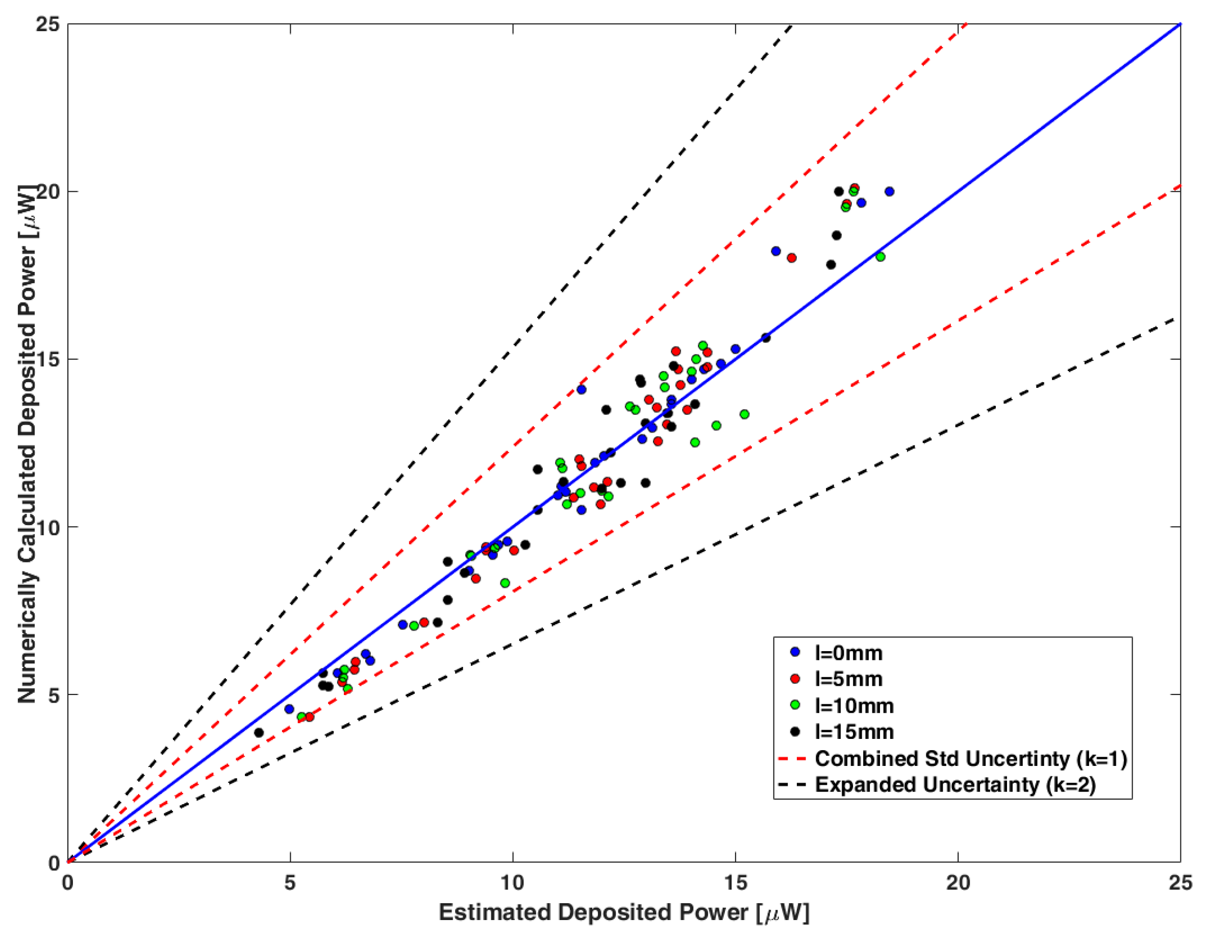
The absorbed power at the tips of the lead pairs was then calculated using the modified Tier 3 process as defined in Equations (3) and (4) for different relative positions. Figure 9 shows the 1:1 plot of the power assessed by the proposed method and the corresponding power calculated from the full-wave simulations for the various lead pair configurations. The maximum deviation between them is less than 0.86 dB, which is the combined standard uncertainty (see Section 3.4). The red and black dashed lines show the combined standard uncertainty (k = 1) and the expanded uncertainty (k = 2), respectively.

3.3. Uncertainty in the Assessment of the Deposited Power and the Temperature Increase

Table S1 in Supplementary Material summarizes the sources of uncertainty and the confidence interval obtained for the different numerical steps of the proposed method. Moreover, Table S2 contains the uncertainty budget for the proposed modified Tier 3 approach. The calculated combined uncertainty (k = 1) and the expanded uncertainty (k = 2) were estimated at 0.86 dB and 1.72 dB, respectively.

3.4. Application of the Modified Tier 3 Process for Various Lead Characteristics

The introduced modified Tier 3 procedure was repeated for different geometrical characteristics and material properties of the leads, as well as material properties of the surrounding tissues, and the absorbed power at their tips was assessed. More specifically, the insulation radius, the lead length and the dielectric characteristics of the medium were varied by ±10% from their initial values, as described in Section 2.1.

Table 3. The deviation in dB of the deposited power at leads with different properties and surrounding tissue as assessed by the full-wave simulations and the proposed approach.

Properties of Configuration		Value	Deviation [dB]
Properties of Lead	Insulation Permittivity	2	0.43
		4	0.47
	Tip Length [mm]	5	0.41
		15	0.32
	Insulation Radius [mm]	0.99	0.34
		0.81	0.37
	Lead Length [cm]	44	0.12
		36	0.10
Properties of Tissue	Dielectric Permittivity	85.8	0.33
		70.2	0.29
	Conductivity [S/m]	0.517	0.40
		0.423	0.38

presents the deviation between the calculated deposited power obtained with electromagnetic simulations and the corresponding deposited power evaluated with our proposed numerical method. This deviation was well within the confidence interval and less than 0.5 dB.

Our process was also applied for a pair of realistic multi-electrode implants, different from the generic leads of uncapped wires studied above. Figure 10a illustrates the SAR distribution at their electrodes. Figure 10b presents the deposited power for each electrode as assessed by the full-wave simulations, the standard Tier 3 approach and the here proposed modified Tier 3 procedure. The deviation between the numerically calculated power from the Sim4Life and the estimated one by the proposed method is in the range of 0.1 to 0.5 dB for the different electrodes. On the contrary, the respective deviation between the simulation results and the values obtained by the standard Tier 3 process ranges from 2.9 to 3.8 dB.

Regarding the placement of leads along trajectories inside a human head, Figure 11 shows the SAR distribution at the tips of the generic implants. The deviation between the numerically calculated induced power at the tips of the pair of leads and that estimated by the proposed approach was 0.2 dB, whereas the difference from the power estimated with the standard Tier 3 procedure was 3.4 dB.

4. Discussion

Based on ISO/TS 10974:2018, an assessment of the enhanced tissue heating due to coupling between leads of close proximity should be performed, but a specific method for this process is not defined. In this study, we performed numerical simulations to estimate the effect of the coupling between two leads on the absorbed power using two identical generic implants of uncapped wires at different distances and tip position offsets. In particular, the full-wave simulations for different configurations of the wire pairs resulted in lower values of the power deposited at the tips compared to the case of the single wire. Moreover, the induced power became lower as the distance between the leads became shorter, and the deviation from the single wire case could become higher than 3 dB. Furthermore, considering the standard Tier 3 process for the assessment of the deposited power at the tips of the coupled implants, using the TF of each wire to assess the deposited power separately resulted in a more than 6 dB overestimation.

It should be noted that the findings of this study, with regard to the low induced power at the tips of the pair of generic implants compared to the single implant, are not representative of all positioning configurations and types of implants. In the study in [44], it was also observed that the coupling between parallel, closely spaced leads had lower induced heating compared to a single lead, and the smaller spacing between the leads resulted in lower lead tip heating. On the other hand, other studies indicated that the presence of a second lead modified the heating profile and could have an unpredictable effect on the induced heating depending not only on the relative placement of the implants but also on the lead structure and the incident electric fields [28,45].

Therefore, there is a need for a systematic method to evaluate the induced heating profile caused by a pair of coupled (due to proximity) implant leads during MRI. To calculate the deposited power at the tips of the coupled leads, we propose a numerical technique based on the Tier 3 approach with a standard uncertainty lower than 1 dB. Initially, the power deposition at the tip of the lead was estimated and then it was converted to temperature increase. We verified this method using electric fields with low correlation among them for different relative placements between the wires, and the resulting deviation between the values from the full-wave simulations and this modified Tier 3 approach was within the confidence interval.

The introduced methodology is based on the additive model of [31], which is an experimental process performed on a parallel couple of cables with constant distance between them. However, our method advances this model, developing an estimation methodology of the coupling factors between the leads and the tangential field along their paths, allowing the calculation of the deposited power for realistic in vivo implant placements and not only for parallel placement of the leads.

The proposed numerical methodology can be performed for various configurations of implant leads, dividing the total process into three discrete steps:

• Excite each lead alone with an iso-electric field and determine the profile of the scattered electric field at the trajectory of the other lead.
• Calculate the TF of each lead in the absence of the second lead. Then, placing the leads in positions similar to those inside the patient, excite each lead separately and acquire the TF of both the excited and the unexcited lead.
• Excite each lead of the pair with an iso-electric field and calculate the induced power caused by the coupling at its tip as well as the other lead, obtaining the respective scaling factors A_ii and A_ij, respectively.

Hence, by applying Equation (4) for the evaluation of the scattering field of each lead at the trajectory of the second lead and combining the above values in Equation (3), the RF power deposition around the tips is assessed.

The suggested numerical technique can be employed for the estimation of the induced power at the tips independently of the lead geometry or the surrounding tissue. However, this study is limited to two leads inside a 1.5 T MRI scanner. Future work is needed to introduce the numerical procedure for three or more leads, as well as for 3 T MRI scanners. Furthermore, future work is needed for the estimation of the temperature increase caused by a pair of implants inside a human body.

5. Conclusions

The technical specification ISO/TS 10974:2018 defines a four-tier approach in order to determine the temperature rise in tissue caused by an AIMD during an MRI scan, but a specific method for this estimation is not defined for the cases of implants with multiple leads or abandoned and retained leads, where coupling between the leads could take place. In this study, the Tier 3 approach was employed for a pair of generic leads placed at various relative positions, and an overestimation of more than 6 dB was obtained in the estimated deposited power at the tips. Therefore, based on the Tier 3 approach, a numerical process was proposed for the evaluation of the induced power at the tips of the two leads in close proximity with a standard uncertainty lower than 1 dB. The proposed approach was implemented also for a pair of realistic multi-electrode leads and in the case of implanted leads inside a realistic human head.

References

- Rezai, A.R.; Baker, K.B.; Tkach, J.A.; Phillips, M.; Hrdlicka, G.; Sharan, A.D.; Nyenhuis, J.; Ruggieri, P.; Shellock, F.G.; Henderson, J. Is Magnetic Resonance Imaging Safe for Patients with Neurostimulation Systems Used for Deep Brain Stimulation? Neurosurgery 2005, 57, 1056–1062. [Google Scholar] [CrossRef] [PubMed]
- Greenspon, A.J.; Patel, J.; Lau, E.; Frisch, D.; Ho, R.; Pavri, B.; Ochoa, J.; Kurtz, S. Trends in permanent pacemaker implantation in The United States 1993–2009: Increasing complexity of patients and procedures. J. Am. Coll. Cardiol. 2012, 59, E703. [Google Scholar] [CrossRef]
- Naehle, C.P.; Zeijlemaker, V.; Thomas, D.; Meyer, C.; Strach, K.; Fimmers, R.; Schild, H.; Sommer, T. Evaluation of Cumulative Effects of MR Imaging on Pacemaker Systems at 1.5 Tesla. Pacing Clin. Electrophysiol. 2009, 32, 1526–1535. [Google Scholar] [CrossRef] [PubMed]
- Dormont, D.; Seidenwurm, D.; Galanaud, D.; Cornu, P.; Yelnik, J.; Bardinet, E. Neuroimaging and Deep Brain Stimulation. Am. J. Neuroradiol. 2009, 31, 15–23. [Google Scholar] [CrossRef]
- Achenbach, S.; Moshage, W.; Diem, B.; Bieberlea, T.; Schibgilla, V.; Bachmann, K. Effects of magnetic resonance imaging on cardiac pacemakers and electrodes. Am. Heart J. 1997, 134, 467–473. [Google Scholar] [CrossRef] [PubMed]
- Shellock, F.G.; Fieno, D.S.; Thomson, L.J.; Talavage, T.M.; Berman, D.S. Cardiac pacemaker: In vitro assessment at 1.5 T. Am. Heart J. 2006, 151, 436–443. [Google Scholar] [CrossRef]
- Sommer, T.; Vahlhaus, C.; Lauck, G.; Smekal, A.V.; Reinke, M.; Hofer, U.; Block, W.; Träber, F.; Schneider, C.; Gieseke, J.; et al. MR Imaging and Cardiac Pacemakers: In Vitro Evaluation and in Vivo Studies in 51 Patients at 0.5 T. Radiology 2000, 215, 869–879. [Google Scholar] [CrossRef] [PubMed]
- Mattei, E.; Triventi, M.; Calcagnini, G.; Censi, F.; Kainz, W.; Mendoza, G.; Bassen, H.I.; Bartolini, P. Complexity of MRI induced heating on metallic leads: Experimental measurements of 374 configurations. Biomed. Eng. Online 2008, 7, 11. [Google Scholar] [CrossRef]
- Luechinger, R.; Zeijlemaker, V.A.; Pedersen, E.M.; Mortensen, P.; Falk, E.; Duru, F.; Candinas, R.; Boesiger, P. In vivo heating of pacemaker leads during magnetic resonance imaging. Eur. Heart J. 2004, 26, 376–383. [Google Scholar] [CrossRef]
- Roguin, A.; Zviman, M.M.; Meininger, G.R.; Rodrigues, E.R.; Dickfeld, T.M.; Bluemke, D.A.; Lardo, A.; Berger, R.D.; Calkins, H.; Halperin, H.R. Modern Pacemaker and Implantable Cardioverter/Defibrillator Systems Can Be Magnetic Resonance Imaging Safe. Circulation 2004, 110, 475–482. [Google Scholar] [CrossRef]
- Calcagnini, G.; Triventi, M.; Censi, F.; Mattei, E.; Bartolini, P.; Kainz, W.; Bassen, H.I. In vitro investigation of pacemaker lead heating induced by magnetic resonance imaging: Role of implant geometry. J. Magn. Reson. Imaging 2008, 28, 879–886. [Google Scholar] [CrossRef] [PubMed]
- Nordbeck, P.; Fidler, F.; Friedrich, M.T.; Weiss, I.; Warmuth, M.; Gensler, D.; Herold, V.; Geistert, W.; Jakob, P.M.; Ertl, G.; et al. Reducing RF-related heating of cardiac pacemaker leads in MRI: Implementation and experimental verification of practical design changes. Magn. Reson. Med. 2012, 68, 1963–1972. [Google Scholar] [CrossRef] [PubMed]
- Langman, D.A.; Goldberg, I.B.; Judy, J.; Paul Finn, J.; Ennis, D.B. The dependence of radiofrequency induced pacemaker lead tip heating on the electrical conductivity of the medium at the lead tip. Magn. Reson. Med. 2011, 68, 606–613. [Google Scholar] [CrossRef]
- Nordbeck, P.; Weiss, I.; Ehses, P.; Ritter, O.; Warmuth, M.; Fidler, F.; Herold, V.; Jakob, P.M.; Ladd, M.E.; Quick, H.H.; et al. Measuring RF-induced currents inside implants: Impact of device configuration on MRI safety of cardiac pacemaker leads. Magn. Reson. Med. 2009, 61, 570–578. [Google Scholar] [CrossRef]
- Amjad, A.; Kamondetdacha, R.; Kildishev, A.V.; Park, S.M.; Nyenhuis, J.A. Power deposition inside a phantom for testing of MRI heating. IEEE Trans. Magn. 2005, 41, 4185–4187. [Google Scholar] [CrossRef]
- Nordbeck, P.; Ritter, O.; Weiss, I.; Warmuth, M.; Gensler, D.; Burkard, N.; Herold, V.; Jakob, P.M.; Ertl, G.; Ladd, M.E.; et al. Impact of imaging landmark on the risk of MRI-related heating near implanted medical devices like cardiac pacemaker leads. Magn. Reson. Med. 2010, 65, 44–50. [Google Scholar] [CrossRef] [PubMed]
- Baker, K.B.; Tkach, J.A.; Phillips, M.D.; Rezai, A.R. Variability in RF-induced heating of a deep brain stimulation implant across MR systems. J. Magn. Reson. Imaging 2006, 24, 1236–1242. [Google Scholar] [CrossRef]
- ISO/TS 10974:2018; Assessment of the Safety of Magnetic Resonance Imaging for Patients with an Active Implantable Medical Device. International Organization for Standardization: Geneva, Switzerland, 2018.
- Park, S.-M.; Kamondetdacha, R.; Nyenhuis, J.A. Calculation of MRI-induced heating of an implanted medical lead wire with an electric field transfer function. J. Magn. Reson. Imaging 2007, 26, 1278–1285. [Google Scholar] [CrossRef]
- Yu, C.M.; Hayes, D.L.; Auricchio, A. Cases in Cardiac Resynchronization Therapy; Elsevier Saunders: Amsterdam, The Netherlands, 2014. [Google Scholar]
- Jiang, Z.; Pajic, M.; Moarref, S.; Alur, R.; Mangharam, R. Modeling and verification of a dual chamber implantable pacemaker. In Tools and Algorithms for the Construction and Analysis of Systems: 18th International Conference, TACAS 2012, Proceedings of the European Joint Conferences on Theory and Practice of Software, ETAPS 2012; Tallinn, Estonia, 24 March–1 April 2012, Proceedings 18; Springer: Berlin/Heidelberg, Germany, 2012; pp. 188–203. [Google Scholar]
- Golestanirad, L.; Kirsch, J.; Bonmassar, G.; Downs, S.; Elahi, B.; Martin, A.; Iacono, M.-I.; Angelone, L.M.; Keil, B.; Wald, L.L.; et al. RF-induced heating in tissue near bilateral DBS implants during MRI at 1.5 T and 3 T: The role of surgical lead management. NeuroImage 2019, 184, 566–576. [Google Scholar] [CrossRef]
- Grill, W.M.; Mortimer, J.T. Neural and connective tissue response to long-term implantation of multiple contact nerve cuff electrodes. J. Biomed. Mater. Res. 2000, 50, 215–226. [Google Scholar] [CrossRef]
- Sawyer-Glover, A.M.; Shellock, F.G. Pre-MRI procedure screening: Recommendations and safety considerations for biomedical implants and devices. J. Magn. Reson. Imaging 2000, 12, 510. [Google Scholar] [CrossRef] [PubMed]
- Golestanirad, L.; Rahsepar, A.A.; Kirsch, J.E.; Suwa, K.; Collins, J.C.; Angelone, L.M.; Keil, B.; Passman, R.S.; Bonmassar, G.; Serano, P.; et al. Changes in the specific absorption rate (SAR) of radiofrequency energy in patients with retained cardiac leads during MRI at 1.5T and 3T. Magn. Reson. Med. 2018, 81, 653–669. [Google Scholar] [CrossRef] [PubMed]
- Langman, D.A.; Goldberg, I.B.; Finn, J.P.; Ennis, D.B. Pacemaker lead tip heating in abandoned and pacemaker-attached leads at 1.5 tesla MRI. J. Magn. Reson. Imaging 2011, 33, 426–431. [Google Scholar] [CrossRef]
- Stijnman, P.; Tokaya, J.; van den Berg, C.; Raaijmakers, A. The Transfer Function for Implanted Wires When a Second Wire Is Near. In Proceedings of the Joint Annual Meeting of ISMRM-ESMRMB, Paris, France, 16–21 June 2018. [Google Scholar]
- Mattei, E.; Gentili, G.; Censi, F.; Triventi, M.; Calcagnini, G. Impact of capped and uncapped abandoned leads on the heating of an MR-conditional pacemaker implant. Magn. Reson. Med. 2014, 73, 390–400. [Google Scholar] [CrossRef] [PubMed]
- Yao, A.; Goren, T.; Samaras, T.; Kuster, N.; Kainz, W. Radiofrequency-induced heating of broken and abandoned implant leads during magnetic resonance examinations. Magn. Reson. Med. 2021, 86, 2156–2164. [Google Scholar] [CrossRef] [PubMed]
- McCabe, S.; Scott, J. A Novel Implant Electrode Design Safe in the RF Field of MRI Scanners. IEEE Trans. Microw. Theory Tech. 2017, 65, 3541–3547. [Google Scholar] [CrossRef]
- Kabil, J.; Felblinger, J.; Vuissoz, P.; Missoffe, A. Coupled transfer function model for the evaluation of implanted cables safety in MRI. Magn. Reson. Med. 2020, 84, 991–999. [Google Scholar] [CrossRef] [PubMed]
- Feng, S.; Qiang, R.; Kainz, W.; Chen, J. A Technique to Evaluate MRI-Induced Electric Fields at the Ends of Practical Implanted Lead. IEEE Trans. Microw. Theory Tech. 2015, 63, 305–313. [Google Scholar] [CrossRef]
- Tsanidis, G.; Samaras, T. Numerical calculation of the radiofrequency transfer function of cochlear implants for assessing deposited power in MRI. Phys. Med. Biol. 2020, 65, 175005. [Google Scholar] [CrossRef]
- Stijnman, P.R.S.; Erturk, M.A.; den Berg, C.A.T.; Raaijmakers, A.J.E. A single setup approach for the MRI based measurement and validation of the transfer function of elongated medical implants. Magn. Reson. Med. 2021, 86, 2751–2765. [Google Scholar] [CrossRef]
- Yao, A.; Zastrow, E.; Kuster, N. Test field diversification method forthe safety assessment of RF-induced heating of AIMDs during 1.5-T MRI. In Proceedings of the 25th Annual Meeting of ISMRM, Honolulu, HI, USA, 22–24 April 2017; Volume 65. [Google Scholar]
- Van Gemert, J.H.F.; Brink, W.; Webb, A.; Remis, R. An Efficient Methodology for the Analysis of Dielectric Shimming Materials in Magnetic Resonance Imaging. IEEE Trans. Med. Imaging 2017, 36, 666–673. [Google Scholar] [CrossRef] [PubMed]
- Golestanirad, L.; Iacono, M.I.; Keil, B.; Angelone, L.M.; Bonmassar, G.; Fox, M.D.; Herrington, T.; Adalsteinsson, E.; LaPierre, C.; Mareyam, A.; et al. Construction and modeling of a reconfigurable MRI coil for lowering SAR in patients with deep brain stimulation implants. NeuroImage 2017, 147, 577–588. [Google Scholar] [CrossRef] [PubMed]
- McElcheran, C.E.; Yang, B.; Anderson, K.J.T.; Golenstani-Rad, L.; Graham, S.J. Investigation of Parallel Radiofrequency Transmission for the Reduction of Heating in Long Conductive Leads in 3 Tesla Magnetic Resonance Imaging. PLoS ONE 2015, 10, e0134379. [Google Scholar] [CrossRef] [PubMed]
- Wang, Y.; Song, S.; Zheng, J.; Wang, Q.; Long, S.A.; Kainz, W.; Chen, J. A Novel Device Model Validation Strategy for 1.5- and 3-T MRI Heating Safety Assessment. IEEE Trans. Instrum. Meas. 2020, 69, 6381–6389. [Google Scholar] [CrossRef]
- Kozlov, M.; Horner, M.; Kainz, W. Modeling radiofrequency responses of realistic multi-electrode leads containing helical and straight wires. Magn. Reson. Mater. Phys. Biol. Med. 2019, 33, 421–437. [Google Scholar] [CrossRef]
- Gosselin, M.-C.; Neufeld, E.; Moser, H.; Huber, E.; Farcito, S.; Gerber, L.; Jedensjö, M.; Hilber, I.; Di Gennaro, F.; Lloyd, B.; et al. Development of a new generation of high-resolution anatomical models for medical device evaluation: The Virtual Population 3.0. Phys. Med. Biol. 2014, 59, 5287–5303. [Google Scholar] [CrossRef]
- Angelone, L.M.; Ahveninen, J.; Belliveau, J.W.; Bonmassar, G. Analysis of the Role of Lead Resistivity in Specific Absorption Rate for Deep Brain Stimulator Leads at 3T MRI. IEEE Trans. Med. Imaging 2010, 29, 1029–1038. [Google Scholar] [CrossRef]
- Cabot, E.; Lloyd, T.; Christ, A.; Kainz, W.; Douglas, M.; Stenzel, G.; Wedan, S.; Kuster, N. Evaluation of the RF Heating of a Generic Deep Brain Stimulator Exposed in 1.5 T Magnetic Resonance Scanners. Bioelectromagnetics 2012, 34, 104–113. [Google Scholar] [CrossRef]
- Hu, W.; Wang, Y.; Wang, Q.; Islam, M.Z.; Tsang, J.; Kainz, W.; Chen, J. RF-Induced Heating for Active Implantable Medical Device with Dual Parallel Leads under, MRI. In Proceedings of the 2021 IEEE International Symposium on Antennas and Propagation and USNC-URSI Radio Science Meeting (APS/URSI), Singapore, 4–10 December 2021; pp. 1041–1042. [Google Scholar]
- Kabil, J.; Missoffe, A.; Vuissoz, P.; Pasquier, C.; Felblinger, J. Quantification and impact of lead coupling on RF-induced heating in MRI. In Proceedings of the ISMRM 25th Annual Meeting, Honolulu, HI, USA, 22–27 April 2017. [Google Scholar]
Figure 1.
The relative position of the two generic implants (a) and SAR distribution at the tips of the couple (b) when only the upper lead was excited by a plane wave (d = 6 mm, l = 0.5 mm).
Figure 2.
The incident electric fields (magnitude and phase) corresponding to the (A) first (B) second (C) third (D) fourth (E) fifth (F) sixth (G) seventh (H) eighth row of the Hadamard matrix.
Figure 3.
The placement of the two realistic implants (a) and the cross-section at the proximal end with the layout of the wires (b).
Figure 4.
Positioning of Duke inside the coil (a) and the generic implants along DBS trajectories (b).
Figure 5.
The amplitude of the TF of the single lead and the TF of the excited lead when in its proximity there is a second lead at various distances (a), and the TF of the unexcited lead (b).
Figure 6.
The SAR distribution at the tip of (A) the single wire and at the tips of the pair of wires for d = 6 mm and (B) l = 0 mm, (C) l = 5 mm, (D) l = 10 mm and (E) l = 15 mm when they are excited by the electrical field shown in the first row of the Hadamard matrix.
Figure 7.
The deviation in dB of the deposited power at the tips of the two generic leads compared to the single lead case for different relative positions between them (see
Figure 1a).
Figure 8.
The deviation in dB between the estimated deposited power using the TF of the single generic lead compared to the corresponding one obtained from the full-wave simulations for l = 0 mm and different distances between the generic leads.
Figure 9.
A 1:1 plot of the deposited power estimated by Equation (3) and the corresponding numerically calculated power obtained through full-wave simulations for the different relative positions between the generic leads of the pair. The blue solid line corresponds to the equivalence of the two quantities. The red and black dashed lines show the combined standard uncertainty (k = 1) and the expanded uncertainty (k = 2), respectively.
Figure 10.
The SAR distribution at the electrodes of the pair of realistic multi-electrode leads (a) and the deposited power at each electrode as assessed by the full-wave simulations, the standard Tier 3 process and the modified Tier 3 approach (b).
Figure 11.
The SAR distribution at the wires placed along realistic paths.