Use of Partial Least Squares Structural Equation Modeling (PLS-SEM) to Improve Plastic Waste Management

Abstract

This paper aims to propose improvements to plastic waste management performance via Partial Least Squares Structural Equation Modeling (PLS-SEM) using a survey’s structured questionnaire and hypothesis testing. The methodology has been applied to the metropolis of Salvador, Brazil’s third most populated city, although it can be used for other cities worldwide. All the indicators, constructs, and hypotheses concerning collection, sorting, and recycling came from a literature review. The dependence of the performance on efficiency, effectiveness, the municipality’s socioeconomic aspects, and the municipality’s infrastructure was evaluated, and both academic and practitioner public representatives were surveyed. Since almost double the minimum number of respondents answered the questionnaire and the PLS-SEM statistics showed that the modeling presents consistency, the discussion is relevant. The final results show that the respondents rated the volume of processing to be slightly more significant than the market maturity for the effectiveness of plastic waste management, which in turn contributes to performance. Once the positive influence of the municipality’s infrastructure on performance has also been verified, the Deposit-Return Systems (DRSs) should be considered for improvement, in addition to an increase in the availability of selective collection systems, contributing to the growth of both the recycling rate and business profitability, reflections of performance.

1. Introduction

This is an extended version of a paper published in the 29th International Joint Conference on Industrial Engineering and Operations Management (IJCIEOM), Lusófona University, Lisbon, Portugal, 28–30 June 2023 [1].

Debates surrounding plastics manufacturing and waste management have intensified due to factors such as the increased use of plastics in recent decades and the consequent rise in plastic waste generation [1].

Table 1. Examples of papers addressing plastic waste management with modeling methods. Source: Adapted from [2,3].

Analysis Type	Authors	Purpose	Country/Region	Method
Qualitative through statistical modeling	[4]	To identify the factors affecting reverse logistics performance	Sri Lanka	PLS-SEM with questionnaire from a literature review
Qualitative through statistical modeling	[5]	To discover the factors influencing consumers’ recycling behavior patterns concerning plastic waste	Pakistan	PLS-SEM with questionnaire from a literature review
Multi-criteria decision-making (MCDM)	[6]	To reduce the accumulation of plastic waste by returning it to recycling	Indonesia	AHP
	[7]	To find a suitable recycling method for managing both disposal and recycling of plastic materials	India	HPF-ELECTRE III, HPF-TOPSlS
Quantitative through mathematical modeling	[8]	To analyze and quantify Brazilian post-consumer plastic packaging waste flows	Brazil	Material flow analysis
	[9]	To combine a green supply chain with a geographic information system to consider the uncertainty of the price of coal and evaluate its effects on the closed-loop supply chain of plastic recycling	China	Mixed integer linear programming (MILP)

shows examples of papers addressing plastic waste management with modeling, as part of the circular economy state-of-the-art.

According to the Waste Hierarchy, despite recycling being preferable over landfilling and disposing as municipal solid waste (MSW) management practices in favor of sustainability [10], open dumps continue to be a key waste disposal method in Brazil, being a significant environmental issue [11]. By 2015, 60% of Brazilian municipalities were still utilizing this approach, even after the deadline set by their solid waste policy (PNRS) to close them [12].

In Salvador, Brazil’s third most populated city, with 2,418,005 inhabitants [13], 16 operational cooperatives are partnering with Limpurb (the public urban cleaning company) [14]. Although the city council had developed a selective collection program, it faced some challenges in maintaining its operation. In 2019, there were 65 voluntary waste disposal points available to the public, and three cooperatives were responsible for receiving, sorting, weighing, and selling the waste [15].

This metropolis had a low collection rate of recyclables in 2017, which was only 0.49% or 4300 tons per year out of the 871,395 tons of MSW collected [16]. The recyclable waste was collected by waste pickers’ associations with the assistance of the city council.

The startup So+ma has already set up 12 collection points in Salvador in partnership with the Secretariat for Sustainability and Resilience (Secis), and more than 736 tons of recyclable materials have already been collected between January and November 2022. Through a benefits program, participants exchange recyclable waste for points that enable them to take training courses, exams, and obtain discounts in supermarkets [17].

Based on the most recent data corresponding to Salvador in a table from the SNIS (the Brazilian information system on sanitation), 72.8% of the population was served daily by mixed collection service and 27.2% was served two or three times a week by Salvador’s city council in 2021 [18], the most recent year with available data.

The problem is that, with all the aforementioned resources, most of the measurement fields concerning the selective collection of recyclable waste in 2021 appear empty in the same SNIS table [18]. Two other fields show extremely low values, as presented in

Table 2. Data concerning selective collection of recyclable waste in 2021. Source: Adapted from [18].

Municipality	Reference Year	CS011—Volume of Recyclable Plastics Recovered	IN030—Coverage Rate of the Door-to-Door Selective Collection Service in Relation to the Municipality’s Urban Population	IN031—Recovery Rate of Recyclable Materials (Except Organic Matter and Rejects) in Relation to the Total Quantity (RDO ¹ + RPU ²) Collected	IN032—Recovered per Capita Mass of Recyclable Materials (Excluding Organic Waste) in Relation to the Urban Population	IN035—Incidence of Plastics in Total Recovered Material	IN054—Per Capita Mass of Recyclable Materials Collected via Selective Collection
Salvador	2021	-	-	0.81	2.47	-	-

¹ RDO (resíduos domiciliares) comes from Brazilian Portuguese and means household waste. ² RPU (resíduos públicos) comes from Brazilian Portuguese and means public waste.

.

The purpose of this work is to demonstrate a PLS-SEM approach with a structured questionnaire in a survey to test hypotheses concerning factors and then qualitatively measure plastic waste management performance, aiming to propose ways to improve it. In the present study, the methodology has been applied for the improvement of the Brazilian metropolis of Salvador, where the survey took place.

The importance of this work is noticed because, in Brazil, a developing country, there is a knowledge gap concerning how to improve plastic waste management performance with statistical modeling. This issue is considered the research question in the current study.

This paper proceeds with the materials and methods (Section 2), results (Section 3), discussion (Section 4) and conclusions (Section 5).

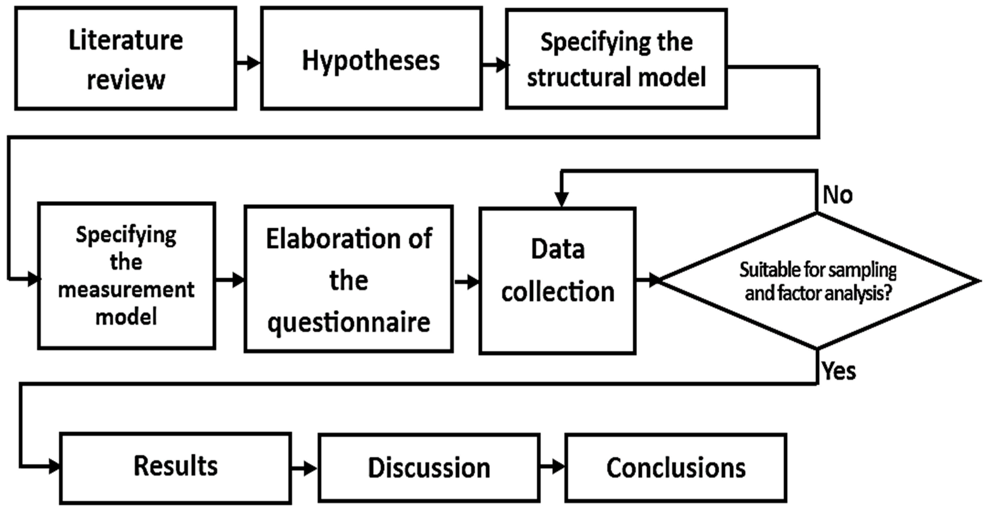
2. Materials and Methods

In the literature review, a search was conducted to find publications that presented discussions of influential factors in plastic waste management. They were grouped by their definition content into constructs. Consequently, each possible relationship between two constructs was hypothesized, giving rise to a structural model.

The methodology steps also include the specification of the measurement model, the elaboration of the questionnaire, data collection, the evaluation of whether or not they are suitable for both sampling and factor analysis, the generation of results, discussion, and conclusions. The sequence is shown as a flowchart in Figure 1.

2.1. The Choice of the PLS-SEM Method for Statistical Modeling

Partial Least Squares Structural Equation Modeling (PLS-SEM) is a robust statistical method that facilitates the examination of hypothetical relationships between factors even in complex models [19,20]. PLS-SEM can be employed even when the collected data do not exhibit a normal (Gaussian) distribution and when the sample size is small (n < 100) [21].

In addition, it enhances the construct reliability and validity, being particularly suitable for models based on composite variables (i.e., constructs) in exploratory studies [22], like the current one, being the reason for such considerations explained in Section 2.5. This is why it has been chosen as the method for this research instead of CB-SEM (Covariance-Based Structural Equation Modeling), which demands confirmatory studies, a normal distribution, and large sample sizes (n > 100) [23].

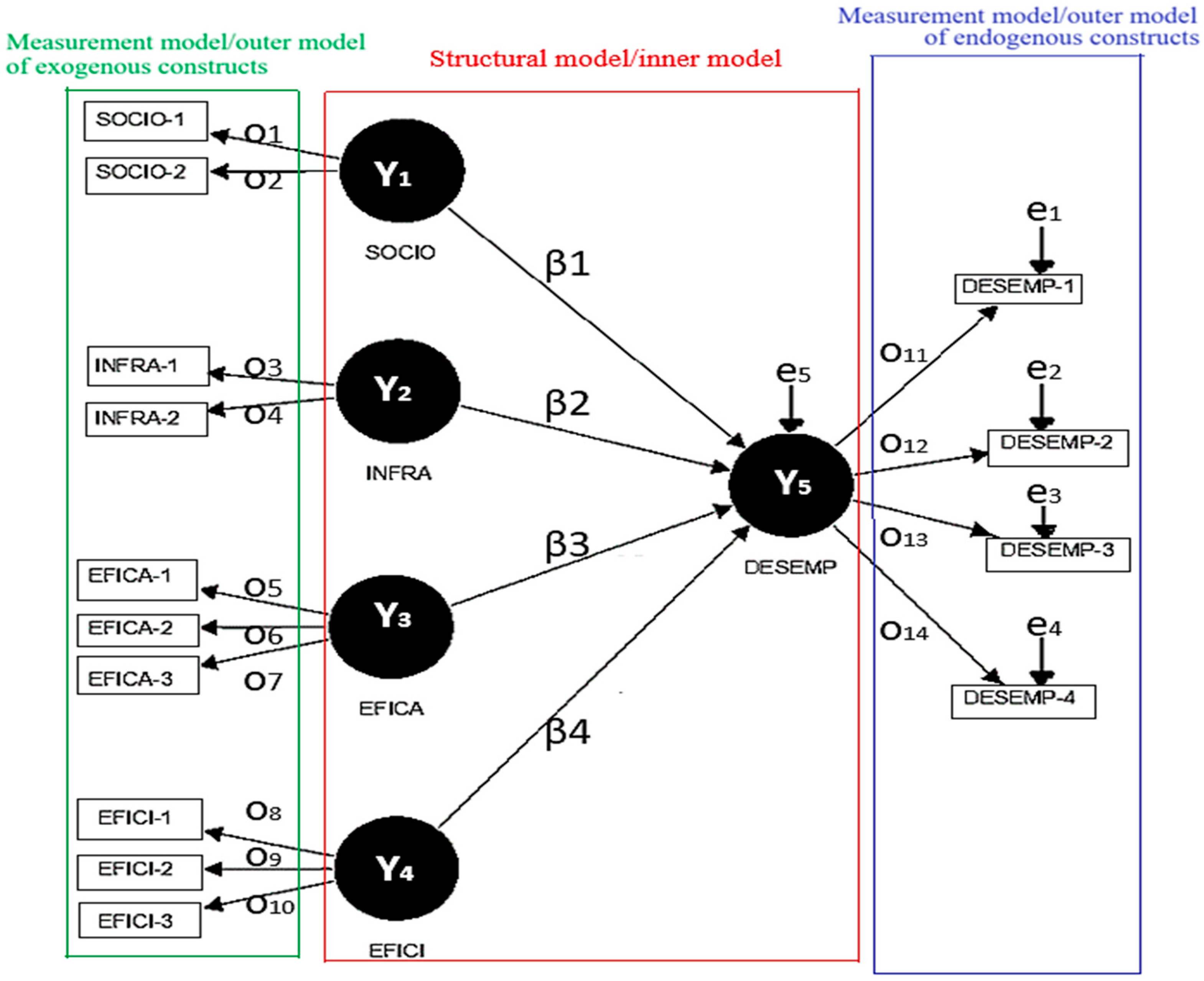
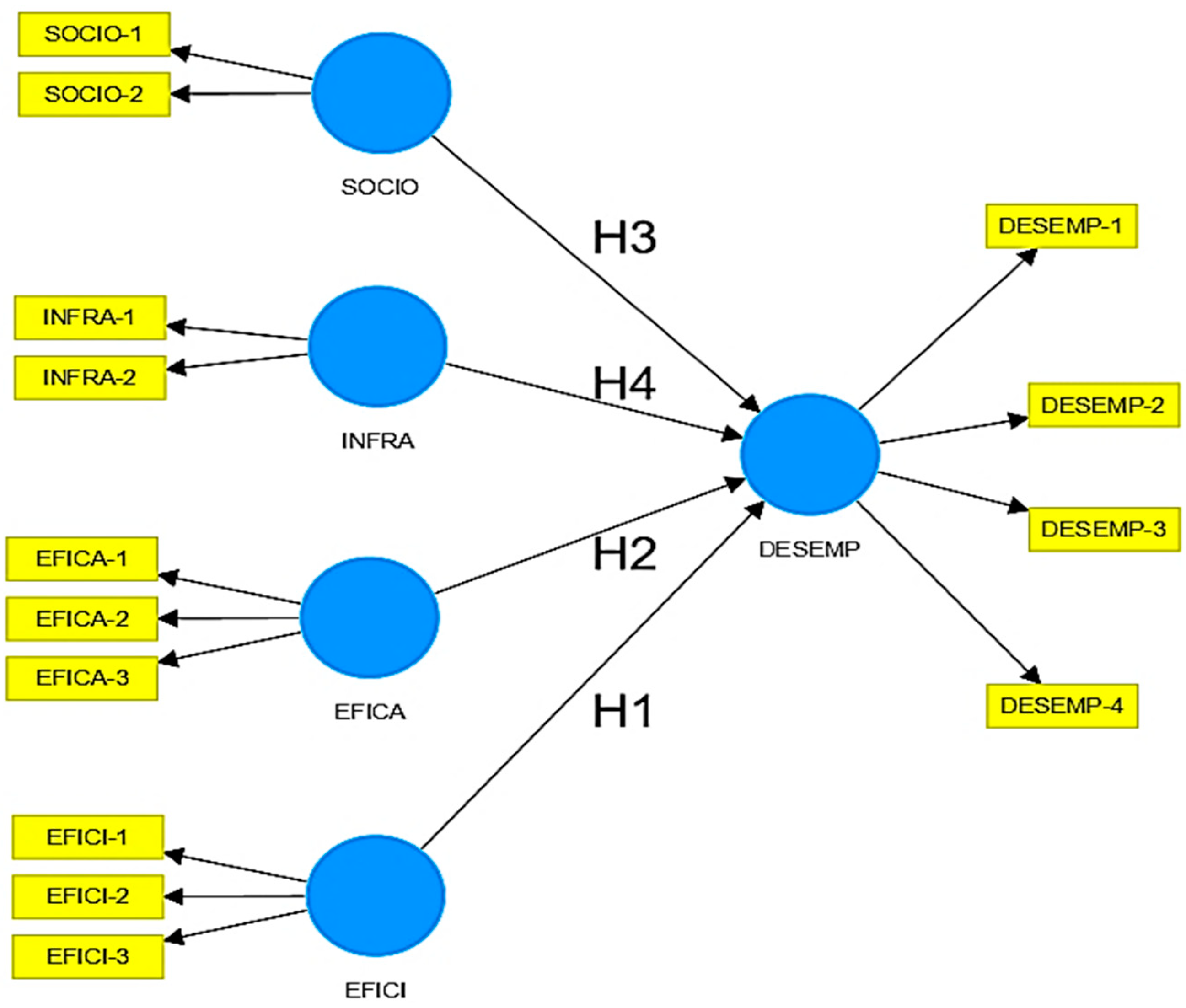
2.2. Specifying the Structural Model

For modeling plastic waste management, four hypotheses (in

Table 3. Hypotheses elaborated with basis on the literature. Source: Adapted from [1].

Hypothesis	Basis
H1: Efficiency positively influences performance	[6,24]
H2: Effectiveness positively influences performance	[24,25]
H3: Municipality’s socioeconomic aspects positively influence performance	[21,26,27]
H4: Municipality’s infrastructure positively influences performance	[28,29]

) were elaborated based on the literature.

A brief description of the hypotheses is provided below.

H1: By optimizing collection networks, and recovering value, efficiency is achieved. This can help companies decrease costs, reduce expenditures, and improve performance [24]. Increasing efficiency leads to a decrease in both plastic waste and pollution. In addition, adopting a sustainability system enables industries to access new markets, thus promoting growth in sales and revenues, and consequently, competitive advantage [6].

H2: The fast handling of collected products, the upgrading of return policies, and the operation of take-back networks enable companies to use the resultant effectiveness to strengthen their competitiveness by increasing consumer confidence in both brand and image [24], which improves performance. The trained employee demonstrates in a company a positive relation between higher performance and effectiveness [25].

H3: Socioeconomic aspects comprise not only income and consumption expenses—which are positively correlated with waste generation—but also the Gross Domestic Product (GDP) [21]. Also, there is a relationship between the growth of the GDP and the increase in the generation of recyclable MSW [26,27]. It is reasonable to think that the bigger the GDP, the greater the positive influence on the performance of plastics if economies of scale are considered.

H4: Improper waste management infrastructure, the application of poor recycling technologies, and a lack of public awareness and incentives result in inefficient and ineffective waste management and disposal [28]. An improved sorting capacity requires additional infrastructure [29].

The performance construct is going to be evaluated concerning its dependence on the other constructs.

2.3. Specifying the Measurement Model

There are reflective and formative PLS measurement models [23]. The reflective scheme aims to verify whether the model explains the real phenomenon via observation since each construct has a direct arrow to the indicator. The accuracy of the model can be assessed using the measurements extracted via observation [23].

The formative scheme minimizes or maximizes a target construct through the relationships between factors present in the model, with the real measurements (indicators) being used as a driver [23].

In

Table 4. Constructs and indicators in the model. Source: Adapted from [1].

Construct	Position in the Model	Indicator	Basis
Efficiency	Exogenous	EFICI-1—Complexity of waste	[28,30]
		EFICI-2—Variety of waste (types of plastic: PET, HDPE, LDPE, PP, PS, PVC, or PUR...)	[30]
		EFICI-3—Variability of waste	[6,30,31]
Effectiveness	Exogenous	EFICA-1—Market maturity	[32,33]
		EFICA-2—Value of waste	[34]
		EFICA-3—Volume of processing	[26]
Performance	Endogenous	DESEMP-1—Recycling rate	[28,35]
		DESEMP-2—Thermochemical conversion rate	[36]
		DESEMP-3—Business profitability	[28,31,37]
		DESEMP-4—Availability of plastics sorting technologies	[38,39]
The infrastructure of the municipality	Exogenous	INFRA-1—Availability of selective collection in the municipality	[8]
		INFRA-2—Availability of Deposit-Return Systems (DRSs)	[40]
Socioeconomic characteristics of the municipality	Exogenous	SOCIO-1—Socioeconomic profile of the municipality	[8]
		SOCIO-2—Population density of the municipality	[41]

, each indicator is followed by the corresponding basis from the literature. To construct the structural model, the fourteen indicators were grouped into five constructs. It is worth noting that regarding the position in the model, an exogenous construct means that it is independent, while an endogenous one is dependent on other constructs.

Remarks from the literature about the indicators are as follows.

EFICI-1. The complexity of plastic packaging shapes contributes to losses in the recycling yield after sorting [30]. Manufacturers using less recyclable or poorly designed materials should pay higher environmental fees [28].

EFICI-2. The diversity of materials in the various plastic layers leads to losses in the recycling yield [30].

EFICI-3. Post-consumer packaging contaminated with food causes losses in the recycling yield [30]. Proper separation and clean disposal of plastics by the population are crucial as the steps before mechanical recycling (the most commonly performed) involving separation, sorting, baling, washing, grinding, composting, and palletizing [6]. Pre-treatment may also be required to remove food residues, for example, in yogurt packaging made of HDPE and margarine packaging made of PP [31].

EFICA-1. Environmental concerns, economic gains, and government regulations drive reverse logistics implementation in the plastic manufacturing industry [32]. Global worries about the future of the Earth and highs in oil prices, such as those observed during the COVID-19 pandemic, elevate the demand for recycled products [33].

EFICA-2. The projection of the plastic waste market and the adoption of biodegradable materials to replace conventional plastics can increase the value of plastic waste [34].

EFICA-3. Economically viable sorting and mechanical recycling of new polymers require scale-up in volumes. As the scale of recycling operations increases, the economics of recycled plastics become more analogous to those of virgin plastics [26].

DESEMP-1. A combination of a high collection rate (83%) and improved recyclability of plastic polymers was found to be the only situation in which the recycling rate reached the European Union’s 55% target for 2030 [28,35].

DESEMP-2. The use of WtE (waste-to-energy) facilities reduces both landfill and open dumps usage and encourages better recycling and MSW (municipal solid waste) management practices in communities nearby, which are more likely to be informed and progressive. As cities with WtE facilities handle the MSW stream more often, they have greater options for recycling. Additionally, on-site materials recovery at the WtE plant can be combined with a municipal recycling program [36].

DESEMP-3. When 40 management scenarios of extended producer responsibility (EPR) for plastic packaging waste generated by Italian households were considered, the likelihood of each polymer being profitable was calculated. Recycling clear and light-blue HDPE, PET, and PP was profitable in above 90% of cases, but mixed-color PET was only profitable in 35% of cases [28]. Economic factors are one of the motivating drivers of reverse logistics because of the potential for profits through recycling and the reduction of costs related to raw materials [37]. Minimizing environmental pollution and enhancing industry profits can come true due to an environmentally friendly waste management system [31].

DESEMP-4. High-tech material recovery facilities (MRFs) utilize advanced technologies, such as eddy currents, magnetic pulleys, optical sensors, and air classifiers, to quicken the separation of unsorted recyclables [38]. Tracer-based sorting (TBS) has the potential to make some sorting and recycling steps obsolete, which can support sustainability and a better circular economy for plastics [39].

INFRA-1. In Brazil, the percentage of plastic packaging waste (PPW) recovered in selective MSW collection (14.4%) was nearly double that of mixed collection (7.3%) in 2017 [8].

INFRA-2. DRSs, as implemented in Sweden, Denmark, and Norway, involve consumers paying an extra deposit because of the packaging when purchasing a drink, and they receive a refund upon returning an empty bottle. These systems have achieved remarkable success, with recycling rates between 85% and 95% of the bottles collected by them [40].

SOCIO-1. In the case of Brazil, for example, although some governments have implemented public policies to overcome the marginalization of waste pickers, there are still many people working in the informal collection sector. The socio-productive inclusion of waste pickers in management systems is fundamental, given that informal collection was 24% higher than the formal selective collection of plastics [8].

SOCIO-2. Das et al. [41] proposed an optimal MSW collection and transportation scheme that minimized the total path length. It was reduced by more than 30% due to the fact of reaching still as many inhabitants but at shorter distances.

2.4. The Choice of the Reflective Measurement Model

A reflective measurement model allows for finding causality flows stemming from the construct to indicators [23]. Reflective indicators can be regarded as a representative subset of all the potential items within the conceptual domain of the construct [23].

Indicators linked to a specific reflective construct should exhibit a high degree of correlation among themselves and be interchangeable. It is acceptable to exclude any single item without modifying the construct’s intended meaning, provided that adequate reliability is maintained.

Figure 2 illustrates this kind of model, with the constructs (Y₁ to Y₅) represented as circles and the indicators as rectangles. Error terms (e₁ to e₄) concerning the DESEMP-1, DESEMP-2, DESEMP-3, and DESEMP-4 indicators indirectly impact the endogenous construct. The structural model includes the error term e₅ concerning the Y₅ endogenous construct [23]. Each outer loading is represented by o_i and each path coefficient by β_i [23].

The reflective structure proposed is shown in Figure 3, with the indicators in rectangles and the constructs in circles.

Among the indicators, one that draws special attention is the profitability resulting from a solution, which has been proposed in the model as a reflection of plastic waste management performance (DESEMP). The basis for that came from another model that used PLS-SEM but for sustainable construction and demolition waste management in Malaysia [42].

2.5. Data Collection, Exploratory Factor Analysis, and the Parameters of the Algorithm Run

The numerical scale of the survey, as well as aspects of the respondent public and the sample size, are discussed in this subsection.

The adoption of a numerical scale for the answer options was needed to facilitate measurement with greater accuracy of non-metric answers. Employing a 5-point scale offered benefits, like a higher explained variance (42.9%) than the 3-point (31.1%) and the 7-point (41.5%) scales in an empirical study [43]. Also, in another study, the 5-point response option produced fairly symmetric and unimodal distributions, differently from the highly skewed J- and U-shaped ones from the 10-point version [44]. In addition, Mirahmadizadeh et al. [45] affirm in a review article that among 60 articles examined, the 5-point scale is the most common. Thus, 5 points have been adopted in the present study.

For the “10-times rule”, the smallest number of respondents should be equal to ten times the largest number of structural paths directed at a construct [46], thus 10 × 4 = 40.

As to the questionnaire distribution, several attempts were made to obtain responses, for example, publication on LinkedIn, private distribution via LinkedIn, and e-mail. They were sequentially tried to obtain a number of respondents that not only met the 10-times rule but also better represented the Salvador metropolis’ order of magnitude. All these tries were very frustrated until it was decided to send the questionnaire privately via a messenger application.

A total of 71 of Salvador’s inhabitants among both the academic and practitioner public agreed to answer. The electronically delivered questionnaire (

Table A1. The questionnaire that was electronically delivered to the respondents.

Part 1—Questions about the respondent’s profile
What is your level of education?		○ Bachelor	○ Specialization			○ Master			○ Doctor
What is the field of study?
How old are you?
Part 2—Questions about plastic waste management
Part 2.1—Efficiency, i.e., fast with less spending of resources
No. (1) High complexity of shape and size of plastic waste.		○ 1-Very bad influence on performance		○ 2	○ 3		○ 4		○ 5-Very good influence on performance.
No. (2) Working with varieties of plastic waste (e.g.,: PET, HDPE, LDPE, PP, PVC, PS) at the same plant facility.		○ 1-Very bad influence on performance.		○ 2	○ 3		○ 4		○ 5-Very good influence on performance.
No. (3) High variability in plastic waste, i.e., the opposite of purity.		○ 1-Very bad influence on performance.		○ 2	○ 3		○ 4		○ 5-Very good influence on performance.
Part 2.2—Effectiveness, i.e., solving the logistics with better safety and better quality
No. (4) Maturity of the plastic waste market.		○ 1-Very low influence on performance.		○ 2	○ 3		○ 4		○ 5-Very high influence on performance.
No. (5) Value of plastic waste.		○ 1-Very low influence on performance.		○ 2	○ 3		○ 4		○ 5-Very high influence on performance.
No. (6) Volume of processing of plastic waste.		○ 1-Very low influence on performance.		○ 2	○ 3		○ 4		○ 5-Very high influence on performance.
Part 2.3—Performance
No. (7) High recycling rate of plastic waste.		○ 1-Very bad influence on performance.		○ 2	○ 3		○ 4		○ 5-Very good influence on performance.
No. (8) High thermochemical conversion rate (for plastics that cannot be recycled but only incinerated).		○ 1-Very bad influence on performance.		○ 2	○ 3		○ 4		○ 5-Very good influence on performance.
No. (9) High profitability of the plastic waste business.		○ 1-Very bad influence on performance.		○ 2	○ 3		○ 4		○ 5-Very good influence on performance.
No. (10) Availability of plastics sorting technologies (e.g.,: automated sorting machines).		○ 1-Very bad influence on performance.		○ 2	○ 3		○ 4		○ 5-Very good influence on performance.
Part 2.4—Infrastructure of the municipality
No. (11) Availability of selective collection in the municipality.		○ 1-Very bad influence on performance		○ 2	○ 3		○ 4		○ 5-Very good influence on performance.
No. (12) Availability of Deposit-Return Systems in the municipality, i.e., vending machines that charge an extra deposit because of the packaging when purchasing a bottled drink, and they get a refund upon returning an empty bottle.		○ 1-Very bad influence on performance.		○ 2	○ 3		○ 4		○ 5-Very good influence on performance.
Part 2.5—Socioeconomic characteristics of the municipality
No. (13) Socioeconomic profile of the municipality.		○ 1-Very low influence on performance.		○ 2	○ 3		○ 4		○ 5-Very high influence on performance.
No. (14) Population density of the municipality.		○ 1-Very low influence on performance.		○ 2	○ 3		○ 4		○ 5-Very high influence on performance.

) collected the respondent’s age, level of education, and field of study in Part 1. A summary of this part’s answers is shown in

Table 5. Summary of respondents’ profile.

Age (Years)	Frequency	Relative Frequency	Field of Study	Frequency	Relative Frequency
<24	16	22.54%	Industrial Engineering	16	22.54%
25–34	39	54.93%	Agricultural Engineering	9	12.68%
35–44	8	11.27%	Administration	7	9.86%
45–54	2	2.82%	Mechanical Engineering	5	7.04%
55–64	3	4.23%	Electrical Engineering	5	7.04%
Unidentified	3	4.23%	Civil Engineering	3	4.23%
			Control and Automation Engineering	2	2.82%
Level of Education	Frequency	Relative Frequency	Sanitary and Environmental Engineering Chemical Engineering	2 2	2.82% 2.82%
Bachelor	37	52.11%	Environmental Analysis	2	2.82%
Specialization Doctor Unidentified	5 12 3	7.04% 16.90% 4.23%	Computer Engineering; Physics; Biology; Mathematics; Architecture; Education and Teaching; Solid Waste; Geography; Nutrition; Environment, Water and Sanitation; Executive Secretariat; Computer Science; Geology; Neurosciences; Education	1 each	1.41% each
			Unidentified	3	4.23%

.

In succession, part 2 of the questionnaire collected their opinions about the degree of each indicator’s positive influence on the performance of collection, sorting, and recycling in Salvador. Electricity generation through waste-to-energy was considered when recycling was not possible. The available answer options ranged from 1 to 5.

The data collected from the respondents are shown in Appendix C,

Table A2. Profiles and answers of the 71 respondents.

Age	Level of Education	Field of Study	EFICI-1	EFICI-2	EFICI-3	EFICA-1	EFICA-2	EFICA-3	DESEMP-1	DESEMP-2	DESEMP-3	DESEMP-4	INFRA-1	INFRA-2	SOCIO-1	SOCIO-2
-	-	-	4	5	3	1	2	4	5	4	4	4	4	4	1	3
-	-	-	2	2	1	5	5	5	4	3	3	5	5	4	5	5
25	Bachelor	Industrial Engineering	3	3	3	2	4	3	3	2	3	2	5	5	3	2
27	Master	Sanitary and Environmental Engineering	3	1	1	4	3	5	3	3	1	3	5	5	5	4
31	Master	Civil Engineering	4	2	2	4	4	3	4	2	4	4	4	4	4	3
31	Master	Chemical Engineering	5	2	1	4	4	3	2	1	2	5	5	5	5	4
33	Specialization 1	Architecture	3	3	3	2	3	3	2	2	3	3	5	4	3	4
28	Master	Solid Waste	4	4	2	2	2	3	4	1	5	5	5	5	3	3
24	Bachelor	Mechanical Engineering	1	1	1	5	5	5	1	1	5	5	3	5	5	5
29	Bachelor	Sanitary and Environmental Engineering	3	3	3	1	1	3	1	3	3	3	3	3	3	3
28	Specialization	Environmental Analyst	2	4	2	4	5	4	4	3	4	4	5	3	4	4
23	Bachelor	Industrial Engineering	3	4	2	5	5	4	3	3	5	3	5	3	4	2
28	Bachelor	Industrial Engineering	1	1	1	1	3	3	3	3	1	4	2	1	4	5
50	Bachelor	Industrial Engineering	3	2	3	5	5	5	5	3	5	5	5	5	4	4
58	Master	Geography	3	2	2	4	3	4	4	3	4	5	5	5	4	3
64	Master	Nutrition	1	1	1	5	5	5	5	5	5	5	5	5	5	3
24	Bachelor	Industrial Engineering	3	1	1	5	5	4	4	1	5	5	5	3	5	5
29	Bachelor	Industrial Engineering	1	2	2	4	4	5	5	4	5	5	5	5	5	3
26	Bachelor	Industrial Engineering	4	3	5	5	2	4	5	2	5	5	5	5	5	5
55	Specialization	Education and Teaching	1	2	1	5	3	5	5	5	5	5	5	5	3	5
33	Master	Electrical Engineering	2	2	2	3	4	3	4	3	3	3	4	4	4	4
28	Bachelor	Mechanical Engineering	2	3	2	3	2	2	3	3	3	3	5	5	4	4
29	Bachelor	Control and Automation Engineering	3	4	3	1	4	2	2	2	4	4	4	5	4	4
24	Bachelor	Industrial Engineering	1	1	1	4	3	5	5	3	3	5	5	5	5	5
20	Bachelor	Agricultural Engineering	2	5	2	5	3	5	5	5	4	5	5	1	4	3
25	Bachelor	Industrial Engineering	2	2	1	4	3	5	5	3	5	5	5	5	5	4
22	Bachelor	Electrical Engineering	4	4	3	4	3	4	4	4	3	4	4	4	3	3
27	Bachelor	Industrial Engineering	5	3	5	3	4	4	3	2	3	2	1	2	3	4
23	Bachelor	Civil Engineering	2	2	1	5	5	5	5	2	5	5	5	4	2	3
23	Bachelor	Agricultural Engineering	1	1	2	5	5	3	5	5	5	5	5	5	5	5
27	Master	Environment, Water and Sanitation	2	3	5	1	1	5	5	5	5	5	3	3	5	5
23	Bachelor	Physics	3	1	4	2	3	5	5	4	3	3	2	1	5	5
32	Doctor	Electrical Engineering	4	3	3	4	2	3	3	2	4	5	5	5	4	2
29	Doctor	Computer Engineering	5	4	4	5	5	5	2	2	5	5	5	5	5	5
28	Bachelor	Electrical Engineering	3	2	1	3	5	5	5	5	5	5	5	5	5	5
35	Bachelor	Control and Automation Engineering	3	5	2	3	5	5	5	3	5	5	5	5	4	4
32	Master	Civil Engineering	2	2	2	5	5	5	5	2	5	5	5	5	4	4
31	Doctor	Geology	5	5	3	5	5	5	5	5	5	5	1	1	3	5
25	Master	Agricultural Engineering	4	3	4	3	2	4	4	2	4	3	4	1	5	5
20	Bachelor	Agricultural Engineering	1	2	2	5	5	5	4	4	5	5	5	4	5	5
20	Bachelor	Agricultural Engineering	4	5	4	4	3	5	3	3	3	4	5	5	5	5
21	Bachelor	Biology	1	3	2	2	3	3	5	4	5	4	5	5	5	5
21	Bachelor	Mathematics	3	3	3	2	3	3	1	1	2	4	1	4	3	3
25	Bachelor	Agricultural Engineering	4	5	2	4	3	4	4	4	4	3	5	5	5	4
34	Bachelor	Mechanical Engineering	3	2	1	4	5	4	5	2	5	5	5	5	4	5
28	Bachelor	Chemical Engineering	3	3	3	4	4	4	4	2	3	4	4	4	4	5
21	Bachelor	Industrial Engineering	3	3	1	5	5	5	5	4	4	5	5	5	5	5
25	Bachelor	Computer Engineering	3	1	1	3	3	3	4	3	5	5	5	4	3	5
24	Bachelor	Industrial Engineering	4	2	2	5	1	4	5	2	5	5	5	5	4	3
25	Bachelor	Mechanical Engineering	2	2	1	3	2	3	3	3	4	5	5	5	4	4
27	Bachelor	Industrial Engineering	3	2	2	5	3	4	5	1	4	5	5	4	5	1
33	Master	Executive Secretariat	3	4	2	2	3	4	4	3	4	3	3	4	3	3
31	Doctor	Neurosciences	1	2	1	5	4	4	5	3	5	4	5	5	4	4
26	Bachelor	Industrial Engineering	1	3	1	5	2	5	5	5	5	5	5	5	4	3
38	Doctor	Administration	5	1	1	3	5	5	5	1	5	5	5	5	5	5
21	Bachelor	Agricultural Engineering	4	3	3	4	3	3	4	3	3	2	4	4	3	3
30	Doctor	Agricultural Engineering	3	3	3	3	3	3	4	4	3	2	5	5	4	2
26	Bachelor	Agricultural Engineering	4	5	4	4	4	3	4	3	4	3	3	3	3	3
46	Doctor	Administration	1	1	1	1	2	2	2	2	1	3	1	2	2	2
25	Bachelor	Electrical Engineering	2	4	3	4	4	3	5	3	4	5	4	4	3	4
37	Master	Industrial Engineering	3	1	1	1	5	3	3	2	4	1	1	1	2	2
26	Doctor	Administration	1	1	1	5	5	5	5	1	5	5	5	5	4	3
33	Master	Mechanical Engineering	1	2	5	1	1	2	2	1	2	1	1	2	3	3
43	Doctor	Administration	2	2	3	5	4	5	4	4	2	4	5	2	5	4
31	Doctor	Administration	2	2	2	5	5	4	5	1	4	5	5	5	5	4
35	Specialization	Administration	1	1	1	4	5	4	3	3	5	5	5	4	4	4
35	Doctor	Administration	5	5	1	4	5	5	5	1	3	5	5	5	3	3
30	Master	Industrial Engineering	3	3	3	3	3	3	3	3	3	3	3	3	3	3
40	Doctor	Education	3	4	3	3	2	2	3	3	2	2	2	2	2	2
39	Specialization	Environmental Analyst	2	2	2	1	3	2	2	1	2	1	2	2	1	2
-	-	-	3	4	2	4	4	5	4	4	5	5	5	5	5	5

¹ Specialization, in Brazil, is a theoretical lato sensu course for professional skills enhancement.

, where each column is a question and each row is a respondent. Only the answers to the 14 questions about plastic waste management, all of them from part 2, were entered into the model as raw data.

As this study is exploratory because it constructs a new model starting from separated indicators and then assesses the contribution of each of them, the p-value criterion of 0.10 was adopted throughout this paper, following the considerations of Hair et al. [23] for studies of this kind.

The Kaiser–Meyer–Olkin (KMO) test was run using the KMO command from the psych library in the RStudio software, 2023.03.0-386 version, to measure the dataset adequacy for sampling [47,48,49]. It yielded a result of 0.738, which was greater than the significance level of 0.10, and thus the dataset is suitable for factor analysis.

With the same library but the cortest.bartlett command, Bartlett’s test of sphericity was conducted to assess their suitability for factor analysis [50]. As the p-value resulted in 1.926 × 10⁻⁴³, it demonstrated significance because it was lower than the significance level of 0.10, with the chi-square test yielding 418.278, and 91 degrees of freedom. The R code that performed both tests is in Appendix A.

These two preliminary findings in the Exploratory Factor Analysis affirm that the dataset was both sufficient and appropriate for conducting a factor analysis, which is going to be presented in Section 3.

The default estimation parameters of the SmartPLS 4 software were kept: all the weights as 1.0; the maximum number of iterations as 300; stop criterion as 10⁻⁷; no use of the Lohmoeller settings; and path as the weighting scheme.

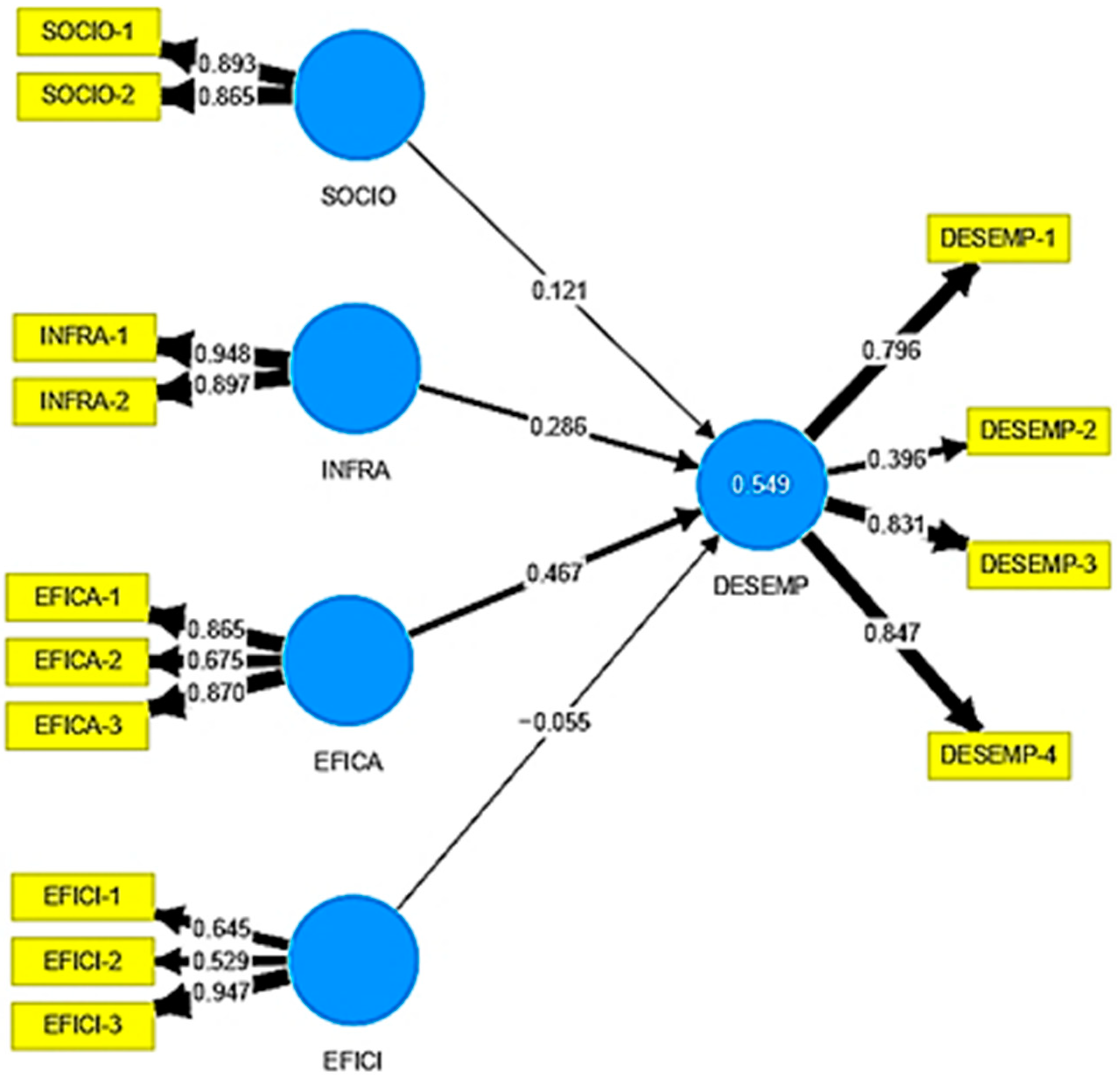
3. Results of the PLS-SEM Path Model Estimation

The PLS-SEM results are discussed in the following subsections.

3.1. Assessing the Initial PLS-SEM Results

A screenshot of the path coefficients and the outer loadings after the initial execution of the PLS-SEM algorithm is shown in Figure 4. The thickness of the arrows is given by the relative values. Indicators are in yellow, and constructs are in blue.

Concerning the outer loading measurements associated with the indicators, it is recommended that they should be at least 0.708 but below 0.95, above which would suggest redundancy and thus diminish the construct validity [23].

The four indicators whose outer loadings were below the threshold were removed and the algorithm was run again. They were EFICI-1 (0.645), EFICI-2 (0.529), EFICA-2 (0.675), and DESEMP-2 (0.396). The other ten outer indicators, for which the outer loadings yielded above 0.708, were held because of their high significance for the model [1]. Figure 5 shows the new path coefficients and outer loadings after the second algorithm run.

3.2. Assessing the PLS-SEM Results of the Reflective Measurement Model

No collinearity problem concerning the outer model was detected. The VIF (variance inflation factor) values ranged from 1.000 to 2.013. Only values of 5.000 or above would indicate a problem [23].

For the assessment of the internal consistency, three criteria must be met. First, each Cronbach’s alpha (CA) measurement should fall above 0.7 but below 0.95. Second, the composite reliability (CR) measurements should exceed 0.7. Third, rho_A, which offers an average value between CA and CR, should be greater than 0.7 [23].

The assessment of convergent validity requires that the average variance extracted (AVE) be greater than 0.5 [23].

Table 6. Outer loadings, Cronbach’s alphas, composite reliabilities, rho_A, and average variance extracted values.

Construct	Indicator	Description	Outer Loading	VIF	Cronbach’s Alpha	CR	rho_A	AVE
DESEMP	DESEMP-1	Recycling rate	0.783	1.489	0.775	0.868	0.798	0.688
	DESEMP-3	Business profitability	0.837	1.752
	DESEMP-4	Availability of plastic sorting technologies	0.866	1.626
EFICA	EFICA-1	Market maturity	0.880	1.508	0.734	0.883	0.737	0.790
	EFICA-3	Volume of processing	0.897	1.508
EFICI	EFICI-3	Variability of waste	1.000	1.000	1.000	1.000	1.000	1.000
INFRA	INFRA-1	Availability of selective collection in the municipality	0.945	2.013	0.830	0.920	0.879	0.852
	INFRA-2	Availability of Deposit-Return Systems	0.901	2.013
SOCIO	SOCIO-1	Socioeconomic profile of the municipality	0.896	1.425	0.706	0.872	0.715	0.772
	SOCIO-2	Population density of the municipality	0.862	1.425

shows all the values.

3.3. Assessing the PLS-SEM Results of the Structural Model

Concerning the assessment of discriminant validity, three criteria are considered. First, no cross-loadings (correlations) with other constructs should be higher or equal to an indicator’s outer loading with its construct. Second, the square root of each construct’s AVE should exceed its highest correlation with any other construct, according to the Fornell–Larcker criterion [51,52]. Lastly, the heterotrait–monotrait ratio (HTMT) of the correlations, representing the ratio of the between-trait correlations to the within-trait correlations, should be below 0.90, but below 0.85 is allowed in cases where the constructs are highly conceptually distinctive in the path model [53].

The HTMT requires the bootstrapping procedure, which assesses the significance of statistics yielded using PLS-SEM and finds out if any unsupported relations exist when the dataset cannot be guaranteed to follow a normal (Gaussian) distribution pattern.

Considering the 14 questions answered by each of the 71 respondents, 994 was the total number of answers. The average option did not concentrate most of the occurrences, as the distribution was: alternative 1 (10.3%), alternative 2 (13.7%), alternative 3 (22.8%), alternative 4 (20.4%), and alternative 5 (32.8%).

The number of bootstrapping samples should be high and at least equal to the number of observations. Each sample from the total of 5000 (SmartPLS 4 default value) contained 71 observations. Thus, 5000 structural models via PLS-SEM were estimated. The confidence interval method was the bias-corrected and accelerated bootstrap, and the test type was two-tailed with a significance level of 0.10 supported by [23].

Table 7. Cross-loadings, Fornell and Larcker’s criterion, and heterotrait–monotrait ratios.

Cross-Loadings (Correlations)
Indicator	DESEMP	EFICA	EFICI	INFRA	SOCIO
DESEMP-1	0.783	0.556	−0.174	0.371	0.270
DESEMP-3	0.837	0.507	−0.162	0.468	0.314
DESEMP-4	0.866	0.649	−0.369	0.580	0.527
EFICA-1	0.594	0.880	−0.249	0.513	0.388
EFICA-3	0.639	0.897	−0.184	0.342	0.519
EFICI-3	−0.298	−0.242	1.000	−0.364	−0.067
INFRA-1	0.603	0.536	−0.359	0.945	0.414
INFRA-2	0.453	0.317	−0.308	0.901	0.282
SOCIO-1	0.433	0.544	−0.094	0.479	0.896
SOCIO-2	0.379	0.346	−0.019	0.181	0.862
Fornell and Larcker’s Criterion
Construct	DESEMP	EFICA	EFICI	INFRA	SOCIO
DESEMP	0.829
EFICA	0.695	0.889
EFICI	−0.298	−0.242	1.000
INFRA	0.581	0.477	−0.364	0.923
SOCIO	0.464	0.513	−0.067	0.386	0.879
Heterotrait–Monotrait (HTMT) Ratio
Construct	DESEMP	EFICA	EFICI	INFRA	SOCIO
DESEMP	1
EFICA	0.911	1
EFICI	0.335	0.296	1
INFRA	0.696	0.597	0.399	1
SOCIO	0.603	0.706	0.151	0.495	1

shows all the values.

In the inner model, there were also no collinearity problems. The VIF values ranged from 1.181 to 1.576. None was 5.000 or above [23].

The coefficient of determination (R²) assesses the explained variance in the dependent (endogenous) constructs caused by all the independent (exogenous) constructs. As a guideline, substantial, moderate, or weak predictive accuracy are respectively indicated by R² values of 0.75, 0.50, or 0.25 [23]. For the performance endogenous construct, it yielded 0.573 for the original R² (statistically meaning the explained variance), and 0.606 for the sample mean R² from the bootstrapping.

Path coefficients (β) play a pivotal role in the evaluation of causal connections between constructs. Path coefficients below 0.10 are not considered statistically significant, while those exceeding 0.20 are typically significant. It is important to note that, at a 10% significance level, the t-value should exceed 1.65 for a two-tailed test, as stipulated by [23].

For assessing the effect of excluding an exogenous construct from the model, the use of the effect size (f²) is necessary, as proposed by [54]. The measurement of each construct can result in small, medium, or large effect sizes, as respectively indicated by values around 0.02, 0.15, or 0.35 [23,46].

Table 8. Decision about the hypotheses considering the VIFs, coefficients of determination (R²), path coefficients (β), effect sizes (f²), standard errors, and t-values.

Hypothesis	VIF	Original R2	Sample Mean 1 R2	Original β	Sample Mean 1 β	Original f²	Sample Mean 1 f²	Standard Error 1	t-Value 2	Decision
H1: EFICI → DESEMP	1.181	0.573	0.606	−0.069	−0.072	0.010	−0.072	0.097	0.717	Not Supported
H2: EFICA → DESEMP	1.576	0.573	0.606	0.493	0.492	0.361	0.492	0.105	4.671	Supported
H3: SOCIO → DESEMP	1.431	0.573	0.606	0.097	0.100	0.015	0.100	0.095	1.026	Not Supported
H4: INFRA → DESEMP	1.485	0.573	0.606	0.283	0.286	0.126	0.286	0.110	2.574	Supported

¹ Bias-corrected and accelerated bootstrapping. ² Statistical significance is confirmed when t-value > 1.65 (p-value < 0.10).

shows all the values, being the sample mean computed considering all the 5000 bootstrapping samples.

According to Table 8, all the exogenous constructs on the left showed a positive influence on performance, except efficiency. The negative sign in the path coefficient for EFICI is an undesired consequence of a mistake. This is explained because its remaining indicator, EFICI-3-variability (impurity), has meaning in itself not beneficial for the performance in the respondents’ opinions as if it were a matter of inefficiency instead of efficiency.

The reader, if they want, is free to think that if inefficiency obtained a coefficient of −0.072, then the correspondence for efficiency is 0.072. Thus, the purity of the waste must favor performance [1]. Similarly, the hypothesis would not be supported, and the indicator’s inherent meaning should be corrected for broader versions of this research in the future.

The hypotheses H2 and H4—respectively, the direct correlation of the EFICA construct on performance, and the direct correlation of the INFRA construct on performance—were supported. H3, related to the municipality’s socioeconomic aspects, could be supported because of its sample mean β of 0.100, but the original β is 0.097 and the t-value is below the threshold. Socioeconomic issues divide opinions and may need a better specification of indicators for conclusive findings.

The Q², also known as predictive relevance or out-of-sample predictive power, measures how well the path model can predict the original values in the dataset. The effect size (q²) compares the relative impact of the constructs’ predictive relevance [23]. The Q² and q² could not be measured in SmartPLS 4 because they are not available in the free version that the authors were able to access until the conclusion of this exploratory study. Instead, the R language in RStudio was used.

R’s seminr library also allows for creating and estimating structural equation models through the command predict_pls. It does not directly calculate the Q² and q² values, but as an alternative approach, it employs both mean absolute error (MAE) and root mean square error (RMSE) predictive statistics. Figure 6 shows the distribution of the prediction errors after running the R code (Appendix D).

In addition, Shmueli et al. [55] recommend using a linear regression model (LM) to generate predictions for the observed variables. As Figure 6 shows, all the skewness printed in the plotting falls between −1 and +1, which is considered excellent [23]. Since no curve is significantly skewed, RMSE should be preferred over MAE in the evaluation [56].

Table 9. PLS and LM out-of-sample metrics.

PLS Out-of-Sample Metrics
	DESEMP_1	DESEMP_3	DESEMP_4
RMSE	1.075	1.023	0.842
MAE	0.826	0.775	0.654
LM Out-of-Sample Metrics
	DESEMP_1	DESEMP_3	DESEMP_4
RMSE	1.107	1.020	0.845
MAE	0.853	0.811	0.658

shows these values.

There is medium predictive power of the supported hypotheses in predicting the DESEMP construct score, according to criteria reported by Danks and Ray [57], because most of the three indicators, exactly two, in the PLS out-of-sample metrics demonstrate lower RMSE values compared to those in LM out-of-sample metrics.

Table 10. Percentage distribution of the indicators by t-value.

Construct	Indicator	Description	Outer Loading	t-Value	Share
Effectiveness (EFICA)	EFICA-1	Market maturity	0.880	22.052	46.4%
	EFICA-3	Volume of processing	0.897	25.480	53.6%
Σ			1.777	47.532	100%
Municipality infrastructure (INFRA)	INFRA-1	Availability of selective collection in the municipality	0.945	22.570	61.7%
	INFRA-2	Availability of Deposit-Return Systems	0.901	13.997	38.3%
Σ			1.846	36.567	100%
Performance (DESEMP)	DESEMP-1	Recycling rate	0.783	10.297	20.4%
	DESEMP-3	Business profitability	0.837	18.968	37.6%
	DESEMP-4	Availability of plastic sorting technologies	0.866	21.189	42.0%
Σ			2.486	50.454	100%

shows the final results, being the indicators’ construct share, by t-value, of the supported hypotheses. The higher the t-value, the greater the significance of the indicator.

Only the supported hypotheses are considered in the discussion to suggest improvements to plastic waste management.

4. Discussion

Since almost double the minimum number of respondents answered the questionnaire and the statistics displayed using SmartPLS 4 showed that the model presents consistency, the discussion is relevant, once most of the respondents have a background in engineering or administration, courses in which concepts related to macroscopic properties and management are covered in greater depth, or chemistry, which provides microscopic notions of the properties of plastics.

A more specialized respondent public, daily involved in the production of plastic and its waste management, is desired to reproduce the methodology in future studies on waste management but including the collection of the position and the time of experience in the area. A semi-structured questionnaire version—which presents not only multiple-choice questions but also open-ended ones—is an additional resource, as respondents would see a greater interaction since they could present opportunities for improvement of plastic waste management in their own words.

It is also worth noting that researchers in qualitative research are moving away from conventional approaches and embracing creative methods, including videoconference interviews [58] and chatbot surveys [59]. The importance of this is that a high participation of the target public can enhance the findings and contribute to a more comprehensive understanding of the subject.

So, from the final results, the following paragraphs discuss the implementation of the results. In this paper, the methodology has been applied to the Brazilian metropolis of Salvador.

Concerning the indicators of the effectiveness construct, most of the respondents considered the volume of processing to be slightly more significant than the market maturity for the effectiveness of plastic waste management, which in turn contributes to performance, as linked to business profitability. This is in line with Adekomaya [26]. However, the market maturity was also judged by them to be significant, which is in line with the study by Dijkstra et al. [60], in which market immaturity is pointed out as a barrier to sustainable plastic waste management.

Once the positive influence of effectiveness on performance has been verified, the maturity of the plastics waste market contributes to more investments in sorting technologies. As the market maturity and volume of processing are reflective indicators of the effectiveness construct, the greater the maturity, the larger the plastic waste volume that can be processed (i.e., recycled). These two indicators also contribute to the increase in both the recycling rate and business profitability, reflections of performance.

In turn, concerning the indicators of the infrastructure construct, the higher significance of the availability of selective collection in this study is a result possibly of the Brazilian respondents’ higher awareness of this facility than of DRS, which in turn has been evaluated as the best disposal method to support the circular economy in India [61].

Once the positive influence of the municipality infrastructure on performance has also been verified, Deposit-Return Systems (DRS)—which have been successful in Nordic countries—may be considered, in addition to an increase in the availability of selective collection systems. These two actions contribute to the growth of both the recycling rate and business profitability, reflections of performance.

These findings reinforce the need to measure and record data for Table 2. This task is assigned to both private and public management, which together can cooperate in the information flow for the evolution of plastic waste management in the municipality.

5. Conclusions

Plastic waste companies that improve their performance achieve a better recycling rate and business profitability. Although the model was developed regarding the infrastructural and socioeconomic issues of the Brazilian metropolis of Salvador, the model can be a basis—which may require adaptations—for other cities worldwide sharing analogous characteristics.

As a methodological contribution, this paper uses PLS-SEM for analyzing the relationships between variables in plastic waste management, which might be of interest to researchers seeking new ways to analyze data. Additionally, this paper offers practical insights, which can benefit the industry, plastic recycling providers, and local governments. The paper’s findings include the detection of factors that influence plastic waste management according to the respondents and the development of a model explaining the relationships between these factors.

As future research, when taking into account the limitations of the current version, the questions related to each indicator should be inherently neutral and the model should have more indicators, constructs, and hypotheses, involving management factors, operation, and matters related to energy and environment. Also, the strengthening of the results of Salvador’s waste pickers should be addressed even if socioeconomic issues need a better specification of indicators for conclusive findings.

References

1. Pereira, L.M.; Freires, F.G.M. Use of Structural Equation Modeling to improve the Plastic Waste Management of a Brazilian capital. In Proceedings of the 29th International Joint Conference on Industrial Engineering and Operations Management (IJCIEOM), Lisbon, Portugal, 28–30 June 2023; Available online: http://portalabepro.educacao.ws/ijcieom/restrito/arquivos/icieom2023/FULL_0032_37760.pdf (accessed on 28 July 2023).
2. Santos, M.R.; Dias, L.C.; Cunha, M.C.; Marques, J.R. Multicriteria Decision Analysis Addressing Marine and Terrestrial Plastic Waste Management: A Review. Front. Mar. Sci. 2022, 8, 747712. [Google Scholar] [CrossRef]
3. Valenzuela, J.; Alfaro, M.; Fuertes, G.; Vargas, M.; Sáez-Navarrete, C. Reverse Logistics Models for the Collection of Plastic Waste: A Literature Review. Waste Manag. Res. 2021, 39, 1116–1134. [Google Scholar] [CrossRef] [PubMed]
4. Thilakarathne, H.G.K.L.S.; Wijayanayake, A.N.; Peter, S. Evaluating the Factors That Affect the Reverse Logistics Performance in Plastic Supply Chain. In Proceedings of the 2022 International Research Conference on Smart Computing and Systems Engineering (SCSE), Colombo, Sri Lanka, 1 September 2022; IEEE: Piscataway, NJ, USA, 2022; pp. 254–261. [Google Scholar]
5. Khan, F.; Ahmed, W.; Najmi, A.; Younus, M. Managing Plastic Waste Disposal by Assessing Consumers’ Recycling Behavior: The Case of a Densely Populated Developing Country. Environ. Sci. Pollut. Res. 2019, 26, 33054–33066. [Google Scholar] [CrossRef] [PubMed]
6. Agustina Hidayat, Y.; Kiranamahsa, S.; Arya Zamal, M. A Study of Plastic Waste Management Effectiveness in Indonesia Industries. AIMS Energy 2019, 7, 350–370. [Google Scholar] [CrossRef]
7. Geetha, S.; Narayanamoorthy, S.; Kureethara, J.V.; Baleanu, D.; Kang, D. The Hesitant Pythagorean Fuzzy ELECTRE III: An Adaptable Recycling Method for Plastic Materials. J. Clean. Prod. 2021, 291, 125281. [Google Scholar] [CrossRef]
8. Pimentel Pincelli, I.; Borges De Castilhos Júnior, A.; Seleme Matias, M.; Wanda Rutkowski, E. Post-Consumer Plastic Packaging Waste Flow Analysis for Brazil: The Challenges Moving towards a Circular Economy. Waste Manag. 2021, 126, 781–790. [Google Scholar] [CrossRef] [PubMed]
9. Ren, H.; Zhou, W.; Guo, Y.; Huang, L.; Liu, Y.; Yu, Y.; Hong, L.; Ma, T. A GIS-Based Green Supply Chain Model for Assessing the Effects of Carbon Price Uncertainty on Plastic Recycling. Int. J. Prod. Res. 2020, 58, 1705–1723. [Google Scholar] [CrossRef]
10. Li, C.H.; Lee, T.T.; Lau, S.S.Y. Enhancement of Municipal Solid Waste Management in Hong Kong through Innovative Solutions: A Review. Sustainability 2023, 15, 3310. [Google Scholar] [CrossRef]
11. Sebrae: Estudo de Mercado–Comércio e Serviços: Reciclagem de Resíduos. Available online: https://www.sebrae.com.br/Sebrae/Portal%20Sebrae/UFs/BA/Anexos/Reciclagem%20de%20res%C3%ADduos%20na%20Bahia.pdf (accessed on 15 December 2022).
12. Nascimento, V.F.; Sobral, A.C.; Fehr, M.; Yesiller, N.; Andrade, P.R.; Ometto, J.P.H.B. Municipal Solid Waste Disposal in Brazil: Improvements and Challenges. Int. J. Environ. Waste Manag. 2019, 23, 300. [Google Scholar] [CrossRef]
13. Instituto Brasileiro de Geografia e Estatística Panorama Do Censo 2022. Available online: https://censo2022.ibge.gov.br/panorama/ (accessed on 25 October 2023).
14. Empresa de Limpeza Urbana de Salvador (Limpurb)-Secretaria de Ordem Pública. Cooperativas e/ou Associações de Catadores de Materiais Recicláveis Cadastradas na Limpurb. Available online: https://limpurb.salvador.ba.gov.br/wp-content/uploads/2023/05/RELACAO-DAS-COOPERATIVAS-Versao-site-16.05.2023.pdf (accessed on 25 October 2023).
15. Almeida, E.; Oliveira, F.; Nascimento, F. Economia Circular em Salvador-BA: Perspectivas para Gestão e Gerenciamento dos Resíduos Sólidos Inorgânicos. In Painel Salvador de Mudança do Clima-Cadernos Temáticos; Prefeitura Municipal de Salvador: Salvador, Brazil, 2020. [Google Scholar]
16. SNIS (Sistema Nacional de Informações Sobre Saneamento): Série Histórica-Ministério do Desenvolvimento Regional. Diagnóstico do Manejo de Resíduos Sólidos Urbanos de 2017. Brasília, 2019. Available online: http://app4.mdr.gov.br/serieHistorica/ (accessed on 17 July 2023).
17. Secretaria Municipal de Inovação e Tecnologia (SEMIT). Casa So+Ma Recolhe Mais de 700 Toneladas de Materiais Recicláveis Em 2022–Secretaria de Comunicação. Available online: https://comunicacao.salvador.ba.gov.br/casa-soma-recolhe-mais-de-700-toneladas-de-materiais-reciclaveis-em-2022/ (accessed on 26 October 2023).
18. SNIS (Sistema Nacional de Informações sobre Saneamento): Série Histórica-Ministério das Cidades. Available online: http://app4.mdr.gov.br/serieHistorica/ (accessed on 30 June 2023).
19. Santana, W.B.; Maués, L.M.F. Environmental Protection Is Not Relevant in the Perceived Quality of Life of Low-Income Housing Residents: A PLS-SEM Approach in the Brazilian Amazon. Sustainability 2022, 14, 13171. [Google Scholar] [CrossRef]
20. Edeh, E.; Lo, W.-J.; Khojasteh, J. Review of Partial Least Squares Structural Equation Modeling (PLS-SEM) Using R: A Workbook; Hair, J.F., Jr., Hult, G.T.M., Ringle, C.M., Sarstedt, M., Danks, N.P., Ray, S., Eds.; Springer: Cham, Switzerland, 2021; p. 197. [Google Scholar] [CrossRef]
21. Bittencourt, E.S. Metabolismo Socioeconômico dos Resíduos Sólidos: Um Modelo de Análise Através de Equações Estruturais de Pneus em fim de Vida. Ph.D. Thesis, Industrial Engineering, Universidade Federal da Bahia, Salvador, Brazil, 2021. [Google Scholar]
22. Dash, G.; Paul, J. CB-SEM vs PLS-SEM Methods for Research in Social Sciences and Technology Forecasting. Technol. Forecast. Soc. Change 2021, 173, 121092. [Google Scholar] [CrossRef]
23. Hair, J.F.; Hult, G.T.M.; Ringle, C.M.; Sarstedt, M. A Primer on Partial Least Squares Structural Equation Modeling (PLS-SEM), 3rd ed.; SAGE: Los Angeles, CA, USA, 2022; ISBN 978-1-5443-9640-8. [Google Scholar]
24. Wondimu, S. Measuring performance of reverse logistics system in pet bottles recovery in EABSCO. Master’s Thesis, Lo-gistics and Supply Chain Management, Addis Ababa University, Addis Ababa, Ethiopia, 2016. [Google Scholar]
25. Filho, J.C.; Nunhes, T.V.; Oliveira, O.J. Guidelines for Cleaner Production Implementation and Management in the Plastic Footwear Industry. J. Clean. Prod. 2019, 232, 822–838. [Google Scholar] [CrossRef]
26. Adekomaya, O.; Majozi, T. Sustainable Management of Plastic Waste: Assessment of Recycled Biodegradable Plastic Market and Projection for the Future. Eng. Appl. Sci. Res. 2020, 47, 216–221. [Google Scholar] [CrossRef]
27. Olivo, F.; Junqueira, M.C.; Furlan, M.B.; Justi, P.A.; De Morais Lima, P. Monetary Losses Caused by the Absence of Packaging Reverse Logistics: Environmental and Economic Impacts. J. Mater. Cycles Waste Manag. 2020, 22, 1801–1817. [Google Scholar] [CrossRef]
28. Andreasi Bassi, S.; Boldrin, A.; Faraca, G.; Astrup, T.F. Extended Producer Responsibility: How to Unlock the Environmental and Economic Potential of Plastic Packaging Waste? Resour. Conserv. Recycl. 2020, 162, 105030. [Google Scholar] [CrossRef]
29. Martin, E.J.P.; Oliveira, D.S.B.L.; Oliveira, L.S.B.L.; Bezerra, B.S. Life Cycle Comparative Assessment of Pet Bottle Waste Management Options: A Case Study for the City of Bauru, Brazil. Waste Manag. 2021, 119, 226–234. [Google Scholar] [CrossRef] [PubMed]
30. Correa, C.A.; De Oliveira, M.A.; Jacinto, C.; Mondelli, G. Challenges to Reducing Post-Consumer Plastic Rejects from the MSW Selective Collection at Two MRFs in São Paulo City, Brazil. J. Mater. Cycles Waste Manag. 2022, 24, 1140–1155. [Google Scholar] [CrossRef]
31. Letcher, T.M. (Ed.) Plastic Waste and Recycling: Environmental Impact, Societal Issues, Prevention, and Solutions; Elsevier: Cambridge, UK, 2020; ISBN 978-0-12-817880-5. [Google Scholar]
32. Streit, A.F.M.; De Santana, M.P.; De Oliveira Júnior, D.L.; Bassaco, M.M.; Tanabe, E.H.; Dotto, G.L.; Bertuol, D.A. Devel-opment of a Pre-Treatment Process of Polymeric Wastes (HDPE, LDPE/LLDPE, PP) for Application in the Qualification of Selectors of Recyclable Materials. Environ. Dev. Sustain. 2022, 24, 6349–6371. [Google Scholar] [CrossRef]
33. Mwanza, B.G.; Mbohwa, C.; Telukdarie, A. Drivers of Reverse Logistics in the Plastic Industry: Producer’s Perspective. In Proceedings of the International Conference on Industrial Engineering and Operations Management, Bogota, Colombia, 25–26 October 2017; IEOM Society International: Southfield, MI, USA, 2017. ISBN 978-1-5323-5943-9. [Google Scholar]
34. Larrain, M.; Van Passel, S.; Thomassen, G.; Van Gorp, B.; Nhu, T.T.; Huysveld, S.; Van Geem, K.M.; De Meester, S.; Billen, P. Techno-Economic Assessment of Mechanical Recycling of Challenging Post-Consumer Plastic Packaging Waste. Resour. Conserv. Recycl. 2021, 170, 105607. [Google Scholar] [CrossRef]
35. European Commission. A European Strategy for Plastics in a Circular Economy; European Union: Brussels, Belgium, 2018; Available online: https://eur-lex.europa.eu/resource.html?uri=cellar:2df5d1d2-fac7-11e7-b8f5-01aa75ed71a1.0001.02/DOC_1&format=PDF (accessed on 30 July 2023).
36. Daaboul, J.; Le Duigou, J.; Penciuc, D.; Eynard, B. Reverse Logistics: Network Design Based on Life Cycle Assessment. In Advances in Production Management Systems. Sustainable Production and Service Supply Chains; Prabhu, V., Taisch, M., Kiritsis, D., Eds.; IFIP Advances in Information and Communication Technology; Springer: Berlin/Heidelberg, Germany, 2013; Volume 414, pp. 450–460. ISBN 978-3-642-41265-3. [Google Scholar]
37. Klinghoffer, N.B.; Castaldi, M.J. (Eds.) Waste to Energy Conversion Technology; Woodhead Publishing Series in Energy; Woodhead Publisher: Oxford, UK, 2013; ISBN 978-0-85709-636-4. [Google Scholar]
38. Rudolph, N.S.; Kiesel, R.; Aumanate, C. Understanding Plastics Recycling: Economic, Ecological, and Technical Aspects of Plastic Waste Handling; Hanser Publishers: Munich, Germany, 2017; ISBN 978-1-56990-676-7. [Google Scholar]
39. Gasde, J.; Woidasky, J.; Moesslein, J.; Lang-Koetz, C. Plastics Recycling with Tracer-Based-Sorting: Challenges of a Potential Radical Technology. Sustainability 2020, 13, 258. [Google Scholar] [CrossRef]
40. Milios, L.; Holm Christensen, L.; McKinnon, D.; Christensen, C.; Rasch, M.K.; Hallstrøm Eriksen, M. Plastic Recycling in the Nordics: A Value Chain Market Analysis. Waste Manag. 2018, 76, 180–189. [Google Scholar] [CrossRef] [PubMed]
41. Das, S.; Bhattacharyya, B.K. Optimization of Municipal Solid Waste Collection and Transportation Routes. Waste Manag. 2015, 43, 9–18. [Google Scholar] [CrossRef] [PubMed]
42. Ghafourian, K.; Kabirifar, K.; Mahdiyar, A.; Yazdani, M.; Ismail, S.; Tam, V.W.Y. A Synthesis of Express Analytic Hierarchy Process (EAHP) and Partial Least Squares-Structural Equations Modeling (PLS-SEM) for Sustainable Construction and Demolition Waste Management Assessment: The Case of Malaysia. Recycling 2021, 6, 73. [Google Scholar] [CrossRef]
43. Aybek, E.C.; Toraman, C. How Many Response Categories Are Sufficient for Likert Type Scales? An Empirical Study Based on the Item Response Theory. Int. J. Assess. Tools Educ. 2022, 9, 534–547. [Google Scholar] [CrossRef]
44. Garratt, A.M.; Helgeland, J.; Gulbrandsen, P. Five-Point Scales Outperform 10-Point Scales in a Randomized Comparison of Item Scaling for the Patient Experiences Questionnaire. J. Clin. Epidemiol. 2011, 64, 200–207. [Google Scholar] [CrossRef]
45. Mirahmadizadeh, A.; Delam, H.; Seif, M.; Bahrami, R. Designing, Constructing, and Analyzing Likert Scale Data. J. Educ. Community Health 2018, 5, 63–72. [Google Scholar] [CrossRef]
46. Hair, J.F.; Hult, G.T.M.; Ringle, C.M.; Sarstedt, M. A Primer on Partial Least Squares Structural Equation Modeling (PLS-SEM), 2nd ed.; SAGE: Los Angeles, CA, USA, 2017; ISBN 978-1-4833-7744-5. [Google Scholar]
47. Kaiser, H.F. A Second Generation Little Jiffy. Psychometrika 1970, 35, 401–415. [Google Scholar] [CrossRef]
48. Kaiser, H.F.; Rice, J. Little Jiffy, Mark Iv. Educ. Psychol. Meas. 1974, 34, 111–117. [Google Scholar] [CrossRef]
49. Cureton, E.E.; D’Agostino, R.B. Factor Analysis, an Applied Approach; Psychology Press: New York, NY, USA, 1983; ISBN 978-1-315-79947-6. [Google Scholar]
50. Bartlett, M.S. The Effect of Standardization on a χ2 Approximation in Factor Analysis. Biometrika 1951, 38, 337. [Google Scholar] [CrossRef]
51. Fornell, C.; Larcker, D.F. Structural Equation Models with Unobservable Variables and Measurement Error: Algebra and Statistics. J. Mark. Res. 1981, 18, 382–388. [Google Scholar] [CrossRef]
52. Chin, W.W. The Partial Least Squares Approach to Structural Equation Modeling. In Modern Methods for Business Research; Psychology Press: London, UK, 1998; p. 448. ISBN 978-1-135-68413-6. [Google Scholar]
53. Dijkstra, T.K.; Henseler, J. Consistent and Asymptotically Normal PLS Estimators for Linear Structural Equations. Comput. Stat. Data Anal. 2015, 81, 10–23. [Google Scholar] [CrossRef]
54. Cohen, J. Statistical Power Analysis for the Behavioral Sciences, 2nd ed.; L. Erlbaum Associates: Hillsdale, NJ, USA, 1988; ISBN 978-0-8058-0283-2. [Google Scholar]
55. Shmueli, G.; Ray, S.; Velasquez Estrada, J.M.; Chatla, S.B. The Elephant in the Room: Predictive Performance of PLS Models. J. Bus. Res. 2016, 69, 4552–4564. [Google Scholar] [CrossRef]
56. Willmott, C.; Matsuura, K. Advantages of the Mean Absolute Error (MAE) over the Root Mean Square Error (RMSE) in Assessing Average Model Performance. Clim. Res. 2005, 30, 79–82. [Google Scholar] [CrossRef]
57. Danks, N.P.; Ray, S. Predictions from Partial Least Squares Models. In Applying Partial Least Squares in Tourism and Hospitality Research; Ali, F., Rasoolimanesh, S.M., Cobanoglu, C., Eds.; Emerald Publishing Limited: Bingley, UK, 2018; pp. 35–52. ISBN 978-1-78756-700-9. [Google Scholar]
58. Khan, T.H.; MacEachen, E. An Alternative Method of Interviewing: Critical Reflections on Videoconference Interviews for Qualitative Data Collection. Int. J. Qual. Methods 2022, 21, 160940692210900. [Google Scholar] [CrossRef]
59. Beam, E.A. Social Media as a Recruitment and Data Collection Tool: Experimental Evidence on the Relative Effectiveness of Web Surveys and Chatbots. J. Dev. Econ. 2023, 162, 103069. [Google Scholar] [CrossRef]
60. Dijkstra, H.; Van Beukering, P.; Brouwer, R. Business Models and Sustainable Plastic Management: A Systematic Review of the Literature. J. Clean. Prod. 2020, 258, 120967. [Google Scholar] [CrossRef]
61. Balwada, J.; Samaiya, S.; Mishra, R.P. Packaging Plastic Waste Management for a Circular Economy and Identifying a Better Waste Collection System Using Analytical Hierarchy Process (AHP). Procedia CIRP 2021, 98, 270–275. [Google Scholar] [CrossRef]
Figure 1. The methodology steps.
Applsci 14 00628 g001
Figure 2. The structure is divided into both a structural model and a reflective measurement model.
Applsci 14 00628 g002
Figure 3. The reflective structure with indicators, constructs, and hypotheses is depicted in SmartPLS 4.
Applsci 14 00628 g003
Figure 4. Values of the initial path coefficients and outer loadings after the first PLS-SEM algorithm run.
Applsci 14 00628 g004
Figure 5. Values of the obtained path coefficients and outer loadings with the second run after the removal of indicators below the outer loading threshold.
Applsci 14 00628 g005
Figure 6. Distribution of the prediction errors concerning each indicator of the endogenous construct.
Applsci 14 00628 g006