Monte Carlo Sampling of Inverse Problems Based on a Squeeze-and-Excitation Convolutional Neural Network Applied to Ground-Penetrating Radar Crosshole Traveltime: A Numerical Simulation Study

Abstract

Monte Carlo-based sampling methods (MCMC) can be used to solve inverse problems affecting ground penetrating radar (GPR) data. However, due to their high computational complexity, they have not been widely used in practical applications. This article uses neural network methods to replace the computationally complex forward problem of Monte Carlo methods. However, the neural network method is an approximation of the accurate formula method, and this may introduce model errors. In order to reduce the impact of model errors, in this study, we incorporate the Squeeze-and-Excitation (SE) attention mechanism into Convolutional Neural Networks (CNN) to further improve the accuracy of the network. Moreover, with the statistical advantages of the MCMC method, model errors can be explained during the inversion process, further reducing their impact. We apply the proposed method to solve the inversion problem of crosshole ground-penetrating radar travel time data. Compared with commonly used approximate forward models, the method proposed in this paper has better accuracy. The results of data experiments indicate that this method can effectively invert the velocity of underground media.

1. Introduction

Ground-penetrating radar (GPR) is an important tool used in shallow geophysical science and technology. It plays an important role in scientific and technological fields such as engineering detection, environmental protection, disaster rescue, and resource exploration that cannot be replaced by other means [1,2,3,4].

The inversion technology of ground-penetrating radar has always been a focus of research. Xue et al. [5] proposed a common offset ground-penetrating-radar signal inversion method based on ray theory that can be used to calculate the relative dielectric constant of underground media through the offset distance between ground-penetrating radar antennas. Zhou Hui et al. [6] used the Maxwell equation to invert the waveforms of ground-penetrating radar signals, performed forward modeling on a known geological model, extracted excitation pulses from the simulation results, and finally used pulse information for signal inversion. Yang Feng et al. [7] applied the tomography imaging method to the ground-penetrating radar detection task, established an underground medium model, and then sliced the model. They used the Least Squares QR (LSQR) algorithm for inversion, resulting in the detection of underground structures in metal-mining areas. Peter et al. [8] used a Tikhonov-regularized pseudo-inverse operator to perform three-dimensional inversion of the soil–air interface.

Mosegaard et al. [9] introduced the extended Metropolis algorithm to sample posterior probability density; this algorithm can sample and solve nonlinear inversion problems. Hansen et al. applied the MCMC algorithm to the inversion of ground-penetrating radar data and conducted extensive research, including analyzing and interpreting the errors of the ray model, reducing the impact of model errors on the inversion results [10,11,12].

In recent years, with the rapid improvement of computer performance, methods for inverting ground-penetrating radar signals through deep learning have developed rapidly. CNNs are widely used in the image field due to their good performance. Zhao Yong et al. [13] designed a self-coding convolutional neural network based on an end-to-end self-coding CNN structure to invert ground-penetrating radar data into an electromagnetic wave velocity model. Ji Yintao et al. [14] designed a PINet inversion network using convolutional and fully connected algorithms to achieve tunnel detection. Su Yi et al. designed an adaptive linear meta neural network for ground-penetrating-radar signal inversion [15]. Liu Bin et al. proposed GPRInvNet based on the DNN architecture in 2019 to map ground-penetrating-radar B-Scan data to the dielectric permittivity map of underground structures, achieving good inversion of complex tunnel lining structures underground [16]. Hansen applied the BP neural network to the inversion of ground-penetrating radar travel time data, attaining efficient and accurate inversion results [17]. Ma Jianwei et al. improved U-Net based on FCN in 2019 to establish a velocity model from seismic record data [18]. Luo Shiguang et al. [19] designed a GPR dimensional transform autoencoder to extract time-domain features of GPR data and then designed GPR-EInet based on a CNN to invert the time-frequency fusion data pertaining to ground-penetrating radar into an underground dielectric permittivity structure. Wang Hui et al. [20] designed a cascaded CNN network to extract features from ground-penetrating-radar B-Scan signals, first removing direct waves and then extracting feature maps using a CNN.

The SE attention module (Squeeze-and-Excitation attention module) is a module used to improve the performance of convolutional neural networks by dynamically adjusting the weights of input feature maps. The core idea of the SE attention module is to recalibrate the features of each channel, enabling the model to focus more on features with important information [21]. One advantage of the SE attention module is that it can adaptively learn the dependencies between different channels, thereby improving the performance of a model. Additionally, the SE attention module can be combined with other attention mechanisms (such as spatial attention and channel attention) to further enhance the performance of a model [22,23].

Based on the above methods, this article combines an SE-CNN with the MCMC method to achieve efficient travel time inversion of ground-penetrating-radar data. Compared with the conventional ray methods, using SE-CNN instead of a forward model offers more advantages in terms of accuracy.

2. Methods

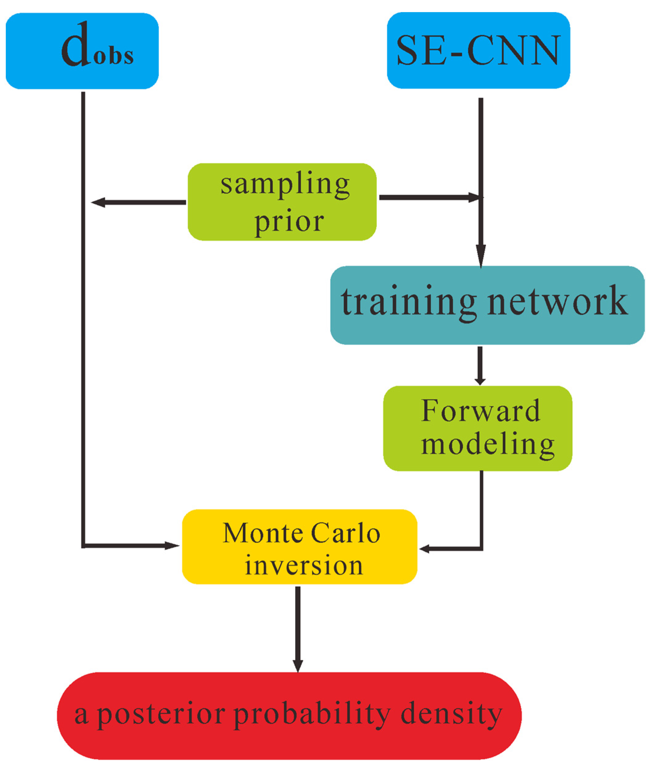
2.1. The Theory of Probability Inversion

Bayesian inversion is based on the Bayesian theorem, which is a statistical method used to update probability estimates based on prior knowledge. In the application of ground-penetrating radar, Bayesian inversion can help to more accurately estimate the characteristics of underground structures, such as soil moisture content, rock type, or other underground features. The Bayesian formula is as follows:

$$P(H|D)=\frac{P(D|H)\times P(H)}{P(D)}$$

(1)

Here, $P(H|D)$ is the posterior probability of hypothesis $H$ given data $D$, $P(D|H)$ is the likelihood of data $D$ given hypothesis $H$, $P(H)$ is the prior probability of hypothesis $H$, and $P(D)$ is the marginal probability of the data.

To solve geophysical inversion problems, considering a probabilistic inversion approach, the respective reverse equation is as follows [24]:

$${\sigma }_M(\mathbf{m})=k{\rho }_M(\mathbf{m})L(\mathbf{m})$$

(2)

Here, ${\sigma }_M(\mathbf{m})$ represents a posteriori probability distribution, which is the solution of the inversion; ${\rho }_M(\mathbf{m})$ represents the prior probability density, denoting the pre-existing knowledge about model attributes; $L(\mathbf{m})$ stands for the likelihood function, which offers a metric illustrating the extent to which the simulated data align with the observed data; and $k$ represents a normalization factor.

The key in this method is to build an appropriate probability model that correlates GPR data with subsurface characteristics. In practical applications, this often involves complex numerical simulations and statistical analysis. For instance, model parameters can be adjusted by comparing actual observational data with model predictions to improve accuracy.

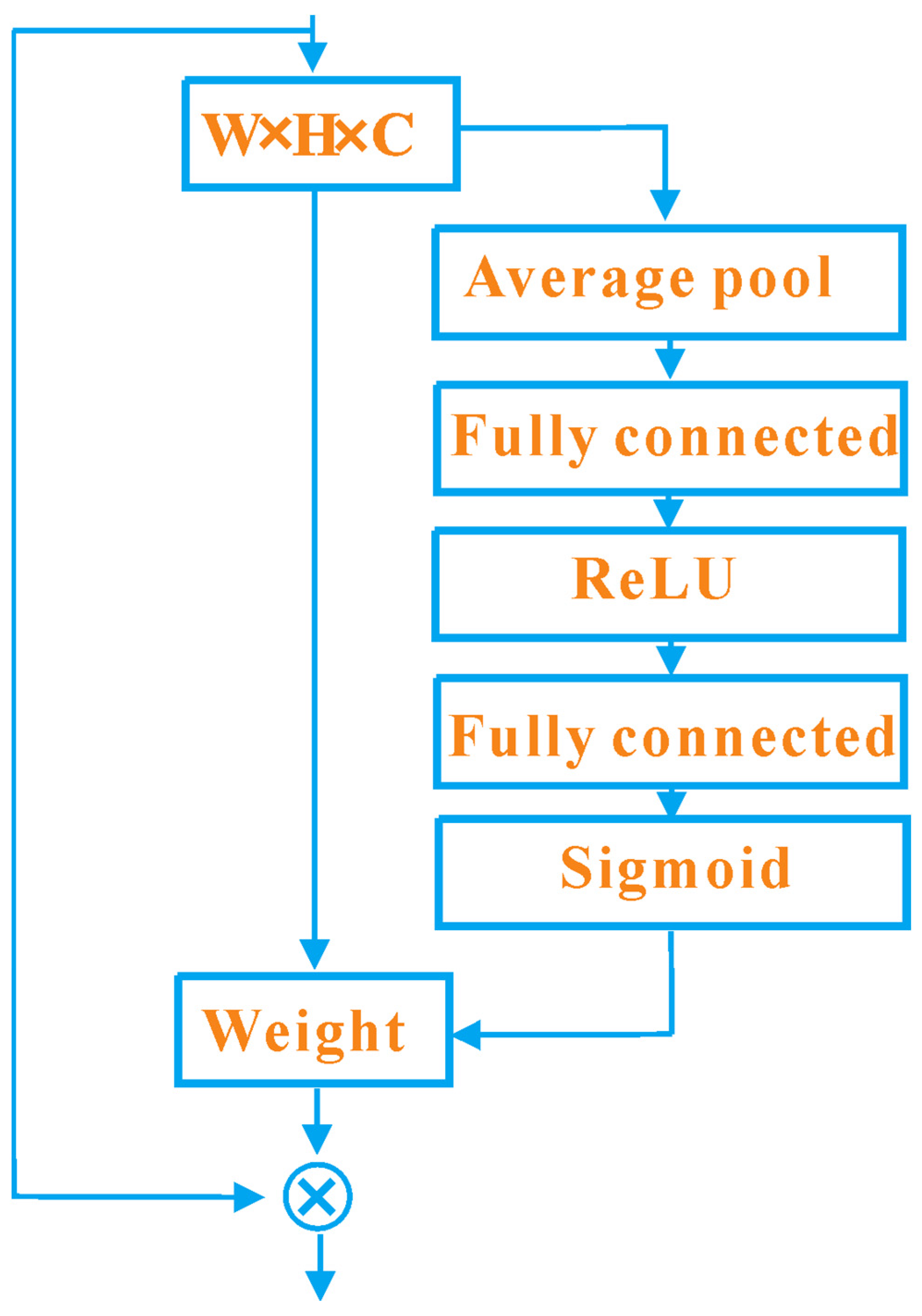
2.2. SE Attention Module

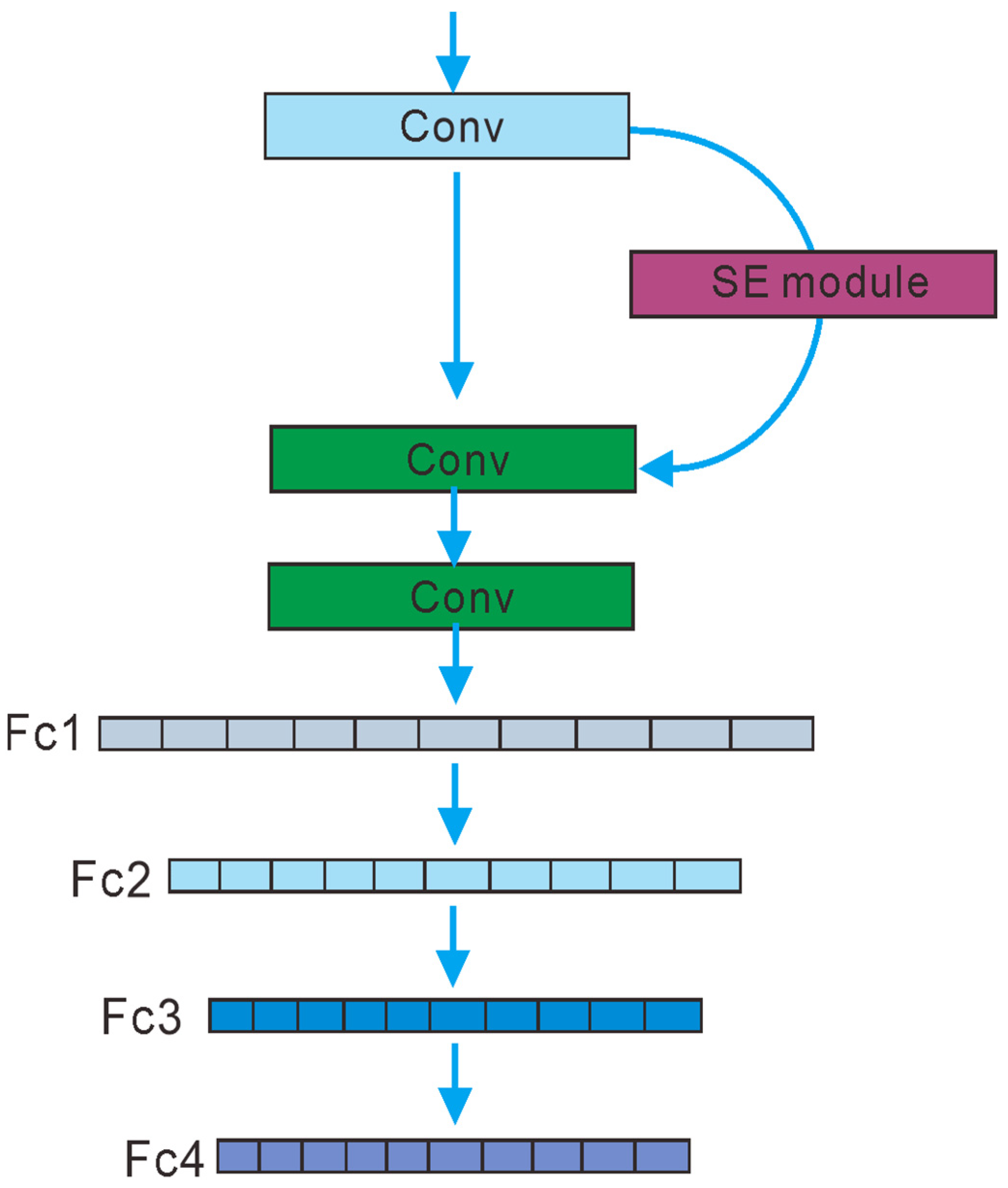
The main components of the SE attention module include global pooling layer, fully connected layer, and Sigmoid activation function. Firstly, the global pooling layer performs global average pooling on the input feature map, resulting in a $1\times 1\times C$ vector, where $C$ represents the number of channels. Then, the fully connected layer maps this vector to a vector with the same number of channels. Finally, the Sigmoid activation function limits the output of the fully connected layer to a value between 0 and 1, resulting in a weight matrix with the same shape as the input feature map. This weight matrix can be seen as a recalibration of the input feature map, guiding the model to focus on features with important information.

Figure 1 shows the SE attention module [9], which mainly consists of squeeze and excitation parts. The main steps of the SE attention module are as follows: first, the squeeze operation is performed. The $W\times H\times C$ feature map is first passed through a dual-channel pooling layer to obtain the global information descriptor of $1\times 1\times C$. After excitation, two fully connected layers are used to predict the importance between channels.

First, the first fully connected layer is scaled through, with the input and output being $1\times 1\times C$ and $1\times 1\times C/r$, respectively, where $r$ is the scaling parameter. Then, the second fully connected layer is cycled through, with the input and output being $1\times 1\times C/r$ and $1\times 1\times C$, respectively.

Afterwards, Sigmaid is used to output vectors of weight values for each layer in the feature map. Finally, there is the scale operation, which multiplies the output weight vector with the feature map to obtain a feature map with weight information. This step focuses on effective features, avoids invalid features, and can better extract target features, all of which can improve the accuracy of the model.

2.3. SE-CNN

SE-CNN is created by inserting SENet modules after the convolutional layer of a CNN. In addition to the local connections and weight-sharing characteristics of a conventional CNN [21], the SENet module can also learn the inter-channel information of a CNN, obtain the weights of each channel, amplify useful feature channels, and suppress channels that have less of an impact on the final task, helping to improve the performance of a CNN [21].

SENet is easy to use, requiring neither a redesign of the network architecture nor an adjustment of hyperparameters. It can be directly inserted into the existing network architecture to form SE-CNN. Moreover, experiments have shown that SENet does not significantly increase model complexity and computational burden [22]. To solve the inversion problem regarding ground-penetrating radar, we designed an SE-CNN, as shown in Figure 2.

From Figure 2, it can be seen that the network is mainly composed of convolutional layers and fully connected layers. The network consists of three convolutional layers, with an SE module added after the first convolutional layer. This network is mainly used for forward simulation of travel time data, so the input of the network is the velocity model of the underground medium, and the output is traveltime data.

The process of the Monte Carlo sampling of inverse problems based on an SE-CNN network is shown in Figure 3. ${\mathrm{d}}_{obs}$ represents observed data. The prior model obtained through sampling can be used to train the SE-CNN network, and the trained network can be used to replace the forward model in Monte Carlo inversion. Finally, by inverting the observed data, ${\mathrm{d}}_{obs}$, a posterior probability distribution can be obtained.

3. Experimental Validation

First traveltime data are among the most commonly used data in inversion problems, involving the propagation of elastic seismic and electromagnetic waves [25,26]. The inverse problem involves inferring information about the velocity field, which leads to the decay of the travel time of a specific phase in the wave field. Here, we consider a traveltime-based inversion problem called “crosshole first arrival time inversion”, which is related to the inversion of the first arrival time delay of the wave field propagating from a set of source positions in one borehole to a set of receiver positions in another borehole. The inverse problem includes inferring the velocity distribution between boreholes. Originally proposed in the context of seismic traveltime data [27], the approach of traveltime inversion has expanded to extensive research into the application of near-surface GPR techniques. The process of inverting crosshole GPR data is recognized as a commonly addressed inverse problem.

In this article, using a multivariate Gaussian probability distribution to generate a reference model $\mathrm{m}$ with a mean velocity of $0.14{ \mathrm{m} \mathrm{ns}}^{-1}$, a variance of $0.000215 {\mathrm{m}}^2{ \mathrm{ns}}^{-2}$, and a spherical covariance model with an isotropic range of $6 \mathrm{m}$, the dimensions of the model are $7\times 13 \mathrm{m}$ ($36\times 66$ pixels with dimensions of $0.2 \mathrm{m}\times 0.2 \mathrm{m}$).

The settings of this recording geometry and parameters are the same as those employed by Hansen et al. (2013) [28], who used two-dimensional finite difference modeling of electromagnetic wave propagation to compute a set of 702 noise-free travel time data via automatic first picking; this method is described by Hansen et al. (2014) [12] and is based on the work of Ernst et al. (2007a,2007b) [29,30] and Cordua et al. (2012) [31]. Uncorrelated zero-mean Gaussian noise with a standard deviation of 0.1 m ns ⁻¹ was added to the noise-free traveltime data, and a reference data set was obtained.

Figure 4 shows the recording geometry and corresponding reference velocity model ${\mathrm{m}}_{\mathrm{ref}}$, with red dots representing the emission source and black dots representing the receiver; the positions of the ND = 702 group source and receiver can be identified by connecting the ray paths. Figure 5 shows the corresponding first-arrival travel time data that were automatically retrieved.

Before inversion, the SE-CNN neural network needed to be trained first. The input of the network is a $36\times 66$ two-dimensional image of the velocity model, and the output is $1\times 702$ one-dimensional travel time data. The input model was obtained by sampling prior information, and the corresponding travel time data were obtained through an accurate but time-consuming 2D FDTD forward mode. In this study, we designed four training datasets with a size of [1000 5000 10,000 20,000], and the corresponding forward models based on the neural network are ${\mathrm{g}}_{1000}$, ${\mathrm{g}}_{5000}$, ${\mathrm{g}}_{10000}$, and ${\mathrm{g}}_{20000}$.

Figure 6 shows four velocity model samples obtained by sampling prior information, and the velocity distribution in the model is random.

After training, we obtained neural network forward models based on different training sizes. Compared with the accurate 2D FDTD model ${\mathrm{g}}_{\mathrm{fd}}$, the forward model based on neural networks has more errors. A sample model was randomly selected to test the forward performance of the neural network model. The forward performance of ${\mathrm{g}}_{1000}$, ${\mathrm{g}}_{5000}$, and ${\mathrm{g}}_{10000}$ is shown in Figure 7. From Figure 7, it can be seen that as the training size increases, the forward modeling of the neural network model becomes more accurate, and ${\mathrm{g}}_{10000}$ is already very similar to the observed data.

The forward-model-simulated results obtained using neural network models ${\mathrm{g}}_{20000}$ and the ray method are shown in Figure 8. Figure 8c shows the residual comparison between forward modeling using neural networks ${\mathrm{g}}_{20000}$ and the ray method. It can be seen that the accuracy of the simulated result based on ${\mathrm{g}}_{20000}$ is superior to that yielded by the ray method.

Errors in forward modeling will affect the inversion results and reduce their accuracy. The MCMC method can be used to statistically analyze the model errors of forward model methods, explain the model errors during the inversion process, and reduce the impact of model errors on the inversion results. In this study, we used 1000 samples to statistically analyze model errors, and the one-dimensional distribution results regarding model errors for different forward models are shown in Figure 9.

To further compare different forward models, Figure 10 shows the covariance matrices corresponding to each forward model. ${\mathrm{g}}_{10000}$ and ${\mathrm{g}}_{20000}$ lead to a less-correlated covariance model as opposed to that obtained using the ray method, as seen in the (lack of) off-diagonal elements of the estimated covariance model.

The posterior probability density function samples obtained by using the trained neural network instead of the forward model and using the Monte Carlo method are shown in Figure 11. In Figure 11, the first model in each row is the reference velocity model, and the remaining four models are samples of a posterior distribution obtained using the corresponding forward-modeling method. The figure shows that as the amount of training increases, the inversion results gradually approach the reference model. This proves the effectiveness of using the SE-CNN neural network method for MCMC inversion.

Figure 12 shows the mean of the posterior distribution samples of the inversion results. From Figure 12, it can be seen that for the mean model, as the training size increases, the details of the mean value of the research results also increases, and it is closer to the reference model. But even for SE-CNN networks with small training sizes, their mean model can still reflect the characteristics of the reference model, such as training sizes of 1000 and 5000.

To further compare the inversion results, we subtracted the mean of the inversion results of each method from the reference model to obtain the corresponding residual distribution, as shown in Figure 13. As the size of the trained neural network increases, the residual gradually decreases, which is consistent with our analysis of the inversion results in Figure 11 and Figure 12.

In order to test the efficiency of the different methods, different forward models were tested with regard to forward time, and the time taken for 100 forward simulations of different forward models was recorded. The results are shown in

Table 1. Computation time analysis of different forward models.

Forward Model	${\mathbf{g}}_{\mathbf{f}\mathbf{d}}$	${\mathbf{g}}_{1000}$	${\mathbf{g}}_{5000}$	${\mathbf{g}}_{10000}$	${\mathbf{g}}_{20000}$	$\mathbf{R}\mathbf{a}\mathbf{y}$
Calculation Time(s)	1015.8	2.03	1.97	1.94	1.92	1.08

. Compared with the most accurate model, both the forward models based on neural networks and that based on the ray method significantly improve computational efficiency. The forward models based on neural networks and the ray method have the same order of magnitude of efficiency, which is three orders of magnitude greater than the accurate forward model.

4. Discussion and Future Work

In this study, we utilized an SE-CNN to invert the travel time data of crosshole ground-penetrating radar and analyzed the error and efficiency of the MCMC inversion method based on network forward models. Based on the work presented in this article, three topics need to be discussed:

(1)

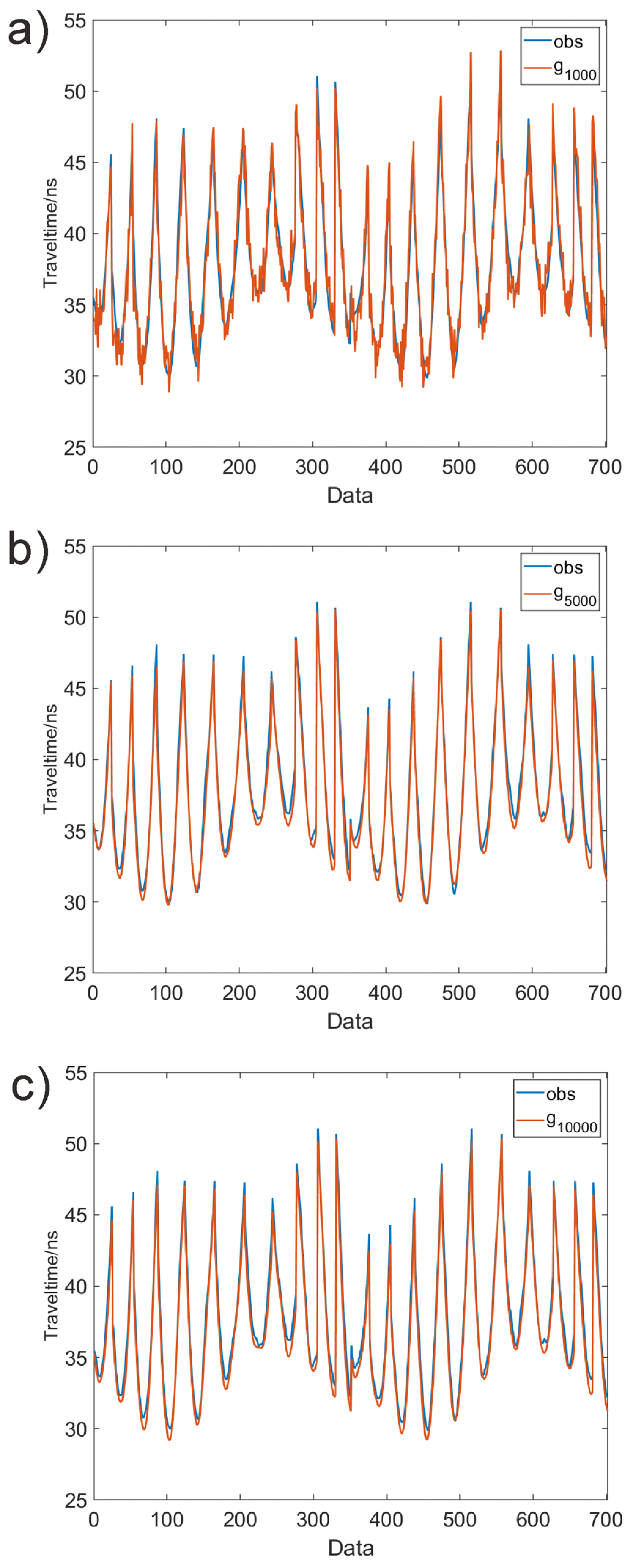
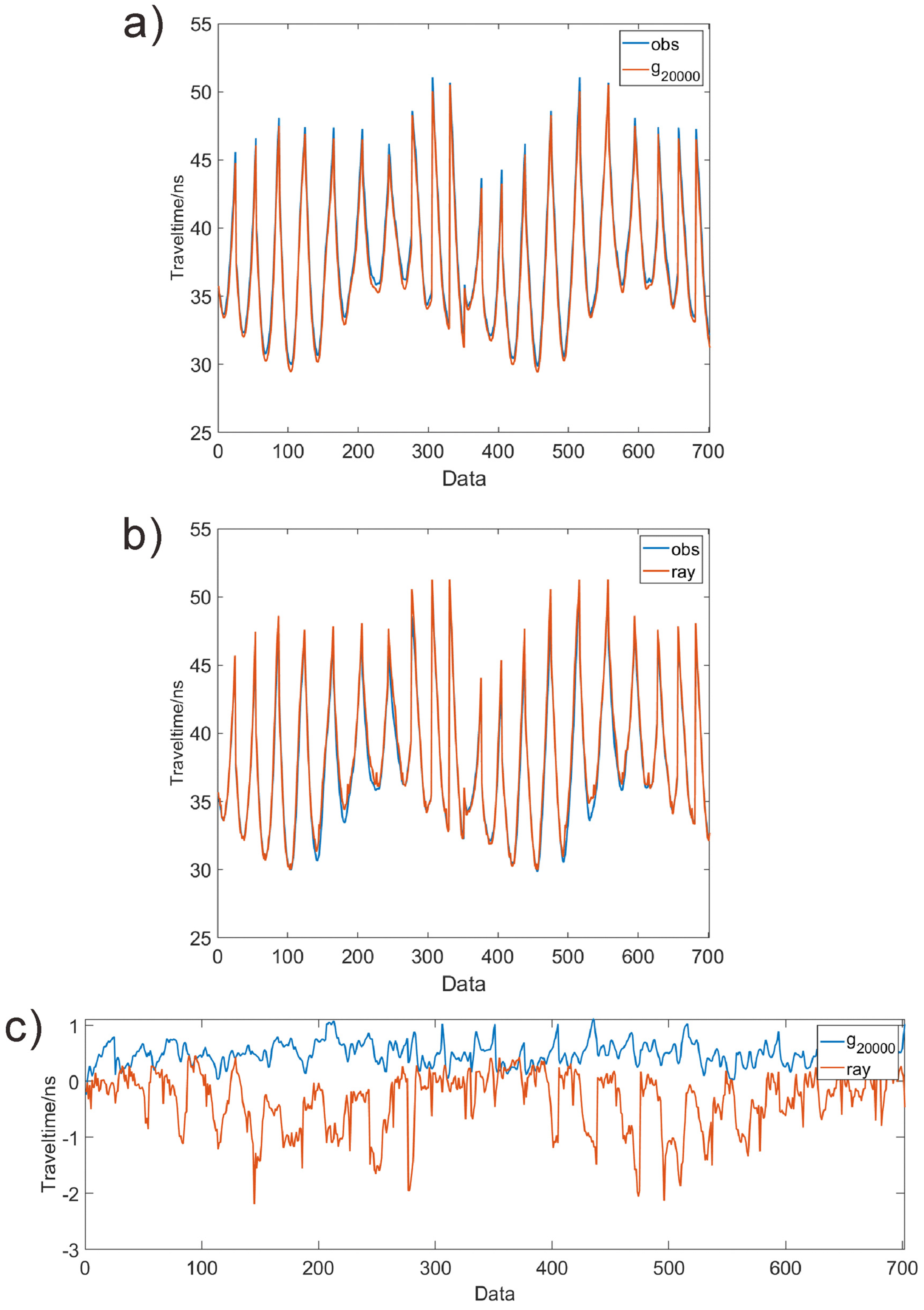
The advantage of an SE-CNN network is that as the training size increases, the number of model errors gradually decreases. A high-precision forward model can be obtained by increasing the training size. The disadvantage is that as the training size increases, the computational cost also increases. Compared with traditional ray methods, the computational efficiencies of both methods are similar, but the model errors of SE-CNN method are smaller when the training size exceeds 20,000.

(2)

At present, the methods of using neural networks for MCMC inversion mainly focus on processing simulated data. The field data quality may not be ideal due to factors such as terrain, geometry systems, and noise. The targeted optimization of network structures is needed. To achieve the application conditions of field data, a large number of field cases need to be analyzed and tested, and this endeavor is a challenge to be addressed in our future research work.

(3)

The attention modules used in this article are SE attention modules. Currently, with the development of neural networks, various attention modules have sequentially emerged. We can try to introduce more types of attention modules into the network model and test their effectiveness. In response to the MCMC inversion problem, the introduction of attention modules not only improves the accuracy of the network but also ensures that the neural network maintains high computational efficiency. Therefore, the design of attention modules and network structures is very important and will be one of the focuses of future research.

5. Conclusions

In this study, we combined an SE-CNN network and the MCMC method to solve the inversion problem of cross hole ground-penetrating-radar data. We replaced the forward model in the MCMC inversion process with an SE-CNN network and used travel time data to invert the underground velocity model. The inversion results indicate that as the training size increases, the accuracy of the inversion results improves.

The advantage of Monte Carlo method is that it can perform statistical analysis on a forward model and explain model errors during the inversion process, which can reduce the impact on the inversion results. By comparing neural network models with different training sizes with the ray method, this article reveals that as the training size of the neural network increases, the accuracy of the forward model increases, and the corresponding model error can be even smaller than the ray method. The error of the neural network model trained 20,000 times in this article is smaller than that obtained using the ray method. In terms of computational efficiency, the forward models based on neural networks and the ray method have the same order of magnitude of efficiency, i.e., three orders of magnitude faster than the accurate forward model. Introducing a SE-CNN network into the MCMC method is an effective way of solving inversion problems, ensuring computational efficiency while obtaining more accurate inversion results.

References

1. Daniels, D. Ground Penetrating Radar, 2nd ed.; IEE: London, UK, 2004. [Google Scholar]
2. Giannopoulos, A. Modelling ground penetrating radar by GprMax. Construct. Building Mater. 2005, 19, 755–762. [Google Scholar] [CrossRef]
3. Meles, G.; Greenhalgh, S.; der Kruk, J.V.; Green, A.; Maurer, H. Taming the non-linearity problem in GPR full-waveform inversion for high contrast media. J. Appl. Geophys. 2012, 78, 31–43. [Google Scholar] [CrossRef]
4. Liu, S.; Lei, L.; Fu, L.; Wu, J. Application of pre-stack reverse time migration based on FWI velocity estimation to ground penetrating radar data. J. Appl. Geophys. 2014, 107, 1–7. [Google Scholar] [CrossRef]
5. Xue, M. Inversion of Common Offset Ground Penetrating Radar Data Based on Ray Theory. Master’s Thesis, Jilin University, Changchun, China, 2021. [Google Scholar]
6. Zhou, H.; Chen, H.; Li, Q.; Wang, J.; Zhang, Q. Ground Penetrating Radar Waveform Inversion Method without Extracting Excitation Pulses. J. Geophys. 2014, 57, 1968–1976. [Google Scholar]
7. Yang, F.; Du, C.; Liang, Y.; Xu, X. Simulation of Metal Mining Exploration Based on Ground Penetrating Radar Wave Velocity Tomography. Prog. Geophys. 2014, 29, 1332–1336. [Google Scholar]
8. Meincke, P. Linear GPR conversion for loose soil and a planar air soil interface. IEEE Trans. Geosci. Remote Sens. 2001, 39, 2713–2721. [Google Scholar] [CrossRef]
9. Mosegaard, K.; Tarantola, A. Monte Carlo sampling of solutions to inverse problems. J. Geophys. Res. 1995, 100, 431–447. [Google Scholar] [CrossRef]
10. Hansen, T.M.; Mosegaard, K.; Cordua, K.S. Using geostatisticsto describe complex a priori information for inverse problems. In VIII International Geostatistics Congress; Ortiz, J.M., Emery, X., Eds.; Geostatistics; University of Chile: Region Metropolitana, Chile, 2008; Volume 1. [Google Scholar]
11. Hansen, T.M.; Mosegaard, K.; Cordua, K.S. Inverse problems with non-trivial priors: Efficient solution through sequential Gibbs sampling: Computational. Geosciences 2012, 16, 593–611. [Google Scholar] [CrossRef]
12. Hansen, T.M.; Cordua, K.S.; Jacobsen, B.H.; Mosegaard, K. Accounting for imperfect forward modeling in geophysical inverse problems-exemplified for crosshole tomography. Geophysics 2014, 79, H1–H21. [Google Scholar] [CrossRef]
13. Zhao, Y. CNN Based Inversion of Ground Penetrating Radar Data and Automatic Recognition of Road Diseases. Master’s Thesis, Jilin University, Changchun, China, 2022. [Google Scholar]
14. Ji, Y. Research on Dielectric Constant Inversion of Ground Penetrating Radar Images Based on Deep Learning. Master’s Thesis, Shandong University, Ji’nan, China, 2021. [Google Scholar]
15. Liu, T.; Su, Y.; Huang, C. Inversion of ground penetrating radar data based on neural networks. Remote Sens. 2018, 10, 730. [Google Scholar] [CrossRef]
16. Liu, B.; Ren, Y.; Liu, H.; Xu, H.; Wang, Z.; Cohn, A.G.; Jiang, P. GPRInvNet: Deep learning based ground penetrating radar data conversion for tunnel liners. IEEE Trans. Geosci. Remote Sens. 2021, 59, 8305–8325. [Google Scholar] [CrossRef]
17. Hansen, T.M.; Cordua, K.S. Efficient Monte Carlo sampling of inverse problems using a neural network-based forward—Applied to GPR crosshole traveltime inversion. Geophys. J. Int. 2017, 211, 1524–1533. [Google Scholar] [CrossRef]
18. Yang, F.; Ma, J. Deep-learning inversion: A next-generation seismic velocity model building methodDL for velocity model building. Geophysics 2019, 84, R583–R599. [Google Scholar] [CrossRef]
19. Luo, S.; Ren, Q.; Wang, C.; Song, Q.; Lei, W. GPR time-frequency domain joint electromagnetic inversion method based on deep learning. J. Radio Wave Sci. 2022, 37, 555–567. [Google Scholar]
20. Wang, H.; Ouyang, X.; Liu, Q.; Liao, K.; Zhou, L. Structural Feature Detection Method for Ground Penetrating Radar 2D Profile Image Based on Deep Learning. J. Electron. Inf. Technol. 2022, 44, 1284–1294. [Google Scholar]
21. Hu, J.; Shen, L.; Sun, G. Squeeze-and-excitation networks. In Proceedings of the IEEE Conference on Computer Vision and Pattern Recognition, Salt Lake City, UT, USA, 18–23 June 2018; pp. 7132–7141. [Google Scholar]
22. Wang, Q.; Wu, B.; Zhu, P.; Li, P.; Zuo, W.; Hu, Q. ECA-Net: Efficient Channel Attention for Deep Convolutional Neural Networks. In Proceedings of the Computer Vision and Pattern Recognition, Seattle, WA, USA, 13–19 June 2019. [Google Scholar]
23. Ba, J.; Mnih, V.; Kavukcuoglu, K. Multiple objectrecognition with visual attention. arXiv 2014, arXiv:1412.7755. [Google Scholar]
24. Tarantola, A.; Valette, B. Inverse problems = quest for information. J. Geophys. 1982, 50, 159–170. [Google Scholar]
25. Bording, R.P.; Gersztenkorn, A.; Lines, L.R.; Scales, J.A.; Treitel, S. Applications of seismic travel-time tomography. Geophys. J. Int. 1987, 90, 285–303. [Google Scholar] [CrossRef]
26. Schuster, G.T.; Quintus-Bosz, A. Wave path eikonal traveltime inversion: Theory. Geophysics 1993, 58, 1314–1323. [Google Scholar] [CrossRef]
27. McMechan, G.A. Seismic tomography in boreholes. Geophys. J. Int. 1983, 74, 601–612. [Google Scholar]
28. Hansen, T.; Cordua, K.; Looms, M.; Mosegaard, K. SIPPI: A Matlab toolbox for sampling the solution to inverse problems with complex prior information: Part 2, Application to cross hole GPR tomography. Comput. Geosci. 2013, 52, 481–492. [Google Scholar] [CrossRef]
29. Ernst, J.; Green, A.; Maurer, H.; Holliger, K. Application of a new 2D time-domain full-waveform inversion scheme to crosshole radar data. Geophysics 2007, 72, J53–J64. [Google Scholar] [CrossRef]
30. Ernst, J.R.; Maurer, H.; Green, A.G.; Holliger, K. Full-waveform inversion of crosshole radar data based on 2-D finite-difference time-domain solutions of Maxwell’s equations. IEEE Trans. Geosci. Remote Sens. 2007, 45, 2807–2828. [Google Scholar] [CrossRef]
31. Cordua, K.S.; Hansen, T.M.; Mosegaard, K. MonteCarlofullwave-form inversion of crosshole GPR data using multiple-point geostatistical a priori information. Geophysics 2012, 77, H19–H31. [Google Scholar] [CrossRef]
Figure 1. Structure diagram of SE attention.
Applsci 14 00618 g001
Figure 2. SE-CNN network structure.
Applsci 14 00618 g002
Figure 3. Process of Monte Carlo sampling of inverse problems based on SE-CNN network.
Applsci 14 00618 g003
Figure 4. Reference model and recording geometry.
Applsci 14 00618 g004
Figure 5. Observation data: 702 travel times.
Applsci 14 00618 g005
Figure 6. (ad) Four different sampling models obtained using prior information.
Applsci 14 00618 g006
Figure 7. (a) Traveltime data simulated based on  g 1000 ; (b) traveltime data simulated based on  g 5000 ; (c) traveltime data simulated based on  g 10000 .
Applsci 14 00618 g007
Figure 8. (a) Traveltime data simulated based on  g 20000 ; (b) traveltime data simulated based on ray method; (c) residual of  g 20000  and ray method.
Applsci 14 00618 g008
Figure 9. 1D distribution of the modeling errors using neural network and ray method.
Applsci 14 00618 g009
Figure 10. (ae) Covariance matrix of five forward methods using trained neural network and ray method.
Applsci 14 00618 g010
Figure 11. (ae) Four samples of the a posterior probability density of the forward models using trained neural network and ray method.
Applsci 14 00618 g011
Figure 12. (af) Means of posterior realizations using trained neural network and ray method.
Applsci 14 00618 g012
Figure 13. (ae) The residual of the inversion results obtained using trained neural network and ray method.
Applsci 14 00618 g013