Abstract
Ground-Based Synthetic Aperture Radar (GBSAR) has non-contact, all-weather, high resolution imaging and microdeformation sensing capabilities, which offers advantages in applications such as building structure monitoring and mine slope deformation retrieval. The Circular Scanning Ground-Based Synthetic Aperture Radar (CS-GBSAR) is one of its newest developed working mode, in which the radar rotates around an axis in a vertical plane. Such nonlinear observation geometry brings the unique advantage of three-dimensional (3D) imaging compared with traditional GBSAR modes. However, such nonlinear observation geometry causes strong sidelobes in SAR images, which makes it a difficult task to extract point cloud data. The Conventional Cell Averaging Constant False Alarm Rate (CA-CFAR) algorithm can extract 3D point cloud data layer-by-layer at different heights, which is time consuming and is easily influenced by strong sidelobes to obtain inaccurate results. To address these problems, this paper proposes a new two-step CFAR-based 3D point cloud extraction method for CS-GBSAR, which can extract accurate 3D point cloud data under the influence of strong sidelobes. It first utilizes maximum projection to obtain three-view images from 3D image data. Then, the first step CA-CFAR is applied to obtain the coarse masks of three-views. Then, the volume mask in the original 3D image is obtained via inverse projection. This can remove strong sidelobes outside the potential target region and obtain potential target area data by intersecting it with the SAR 3D image. Then, the second step CA-CFAR is applied to the potential target area data to obtain 3D point clouds. Finally, to further eliminate the residual strong sidelobes and output accurate 3D point clouds, the modified Density-Based Spatial Clustering of Applications with Noise (DBSCAN) clustering algorithm is applied. The original DBSCAN method uses a spherical template to cluster. It covers more points, which is easily influenced by the strong sidelobe. Hence, the clustering results have more noise points. Meanwhile, modified DBSCAN clusters have a cylindrical template to accommodate the data’s features, which can reduce false clustering. The proposed method is validated via real data acquired by the North China University of Technology (NCUT)-developed CS-GBSAR system. The laser detection and ranging (LiDAR) data are used as the reference ground truth to demonstrate the method. The comparison experiment with conventional method shows that the proposed method can reduce 95.4% false clustered points and remove the strong sidelobes, which shows the better performance of the proposed method.
1. Introduction
Ground-Based Synthetic Aperture Radar (GBSAR) is a new SAR measurement technology that enables acquiring SAR data via a fixed length of linear track [1,2,3]. Its non-contact, all-weather and flexible stationing capabilities offer advantages over traditional spaceborne and airborne platforms, making it more flexible and cost-effective for several applications. With its high precision of repeated path SAR data acquisition, GBSAR has found its usage in monitoring small deformations of landslides, bridges, and buildings [4,5,6]. However, the current linear track GBSAR can only generate two-dimensional (2D) SAR images, as the layover effect means it cannot retrieve 3D deformation information [7,8].
Circular Scanning Ground-Based Synthetic Aperture Radar (CS-GBSAR) is a novel system of GBSAR, which adopts an airborne circular SAR mode into the ground-based platform. It creates a 2D circular synthetic aperture with the antenna rotating on the vertical plane, and makes it capable of 3D imaging on buildings or other scenes with changing altitude [9,10,11,12]. However, the curved observation geometry of CS-GBSAR causes the strong sidelobes in 3D images. As a result, the strong sidelobe diffuses throughout the 3D SAR data, which interferes with adjacent weak targets’ main lobe at different heights. This interference leads to the loss of target detection, thereby causing difficulty in accurately extracting target point clouds in 3D SAR images. Currently, to the best of our knowledge, there exists no effective method for extracting target point clouds from 3D SAR images. One feasible idea to obtain the point cloud is first using a Constant False Alarm Rate (CFAR) detector at different heights to obtain potential point clouds, then extract the exact points with a clustering method such as Density-Based Spatial Clustering of Applications with Noise (DBSCAN).
CFAR has an adaptive threshold detection ability and can adapt to changes in background clutter [13]. It is first applied to detect targets in range profiles. Later, Lincoln Laboratory extended the Two-Parameter CFAR detector to process SAR images in two dimensions [14,15,16], it is now a relatively matured method in 2D SAR images. While implementing the two-parameter CFAR algorithm for target detection, it is essential to detect each layer within the 3D image at varying altitudes. Unfortunately, the diffused 3D strong sidelobes have an influence on detection results, leading to many false detections. To extract point clouds and suppress false detections, the widely applied DBSCAN method can be adopted [17,18,19,20]. Utilizing this algorithm has numerous advantages, including generating cluster for any shape and effectively eliminating outliers in data. However as shown in this paper, the conventional DBSCAN using a spherical template has poor clustering performance. To accurate extract points and exclude the false detection of the sidelobes, the template’s shape should consider the data’s own unique characteristics.
To deal above issues in the extraction of 3D point clouds from CS-GBSAR, this paper proposes a new two-step CFAR-based 3D point cloud extraction method. It is a general method that can handle the CS-GBSAR’s data processing in 3D point cloud extraction applications. It first utilizes maximum projection to obtain three-view images from 3D image data. Then, the first step Conventional Cell Averaging Constant False Alarm Rate (CA-CFAR) is applied to obtain the coarse masks of the three-views. Then, the volume mask in the original 3D image is obtained via inverse projection. This can remove strong sidelobes outside the potential target region and obtain potential target area data by intersecting it with the SAR 3D image. Then, the second step CA-CFAR is applied to potential target area data to obtain 3D point clouds. Finally, to further eliminate the residual strong sidelobes and output accurate 3D point clouds, the modified DBSCAN clustering algorithm is applied. The modified DBSCAN clusters with cylindrical template to accommodate the data’s feature rather than original spherical template, which can reduce false clustering.
The remainder of this paper is structured as follows: Section 2 is the material and dataset. Section 3 introduces details of the proposed method. In Section 3, the CA-CFAR detection algorithm and the conventional DBSCAN clustering algorithm are introduced. On this basis, the methods proposed in this paper are introduced, including the two-step CFAR algorithm and the improved DBSCAN algorithm. Section 4 is the real data experiment, which gives detailed results of each step to validate the method. Section 5 is the discussion, which presents the method comparison experiment to prove the necessity of the proposed method. This section presents the results of the two-step CFAR and conventional method, in addition to the results of original DBSCAN and proposed modified DBSCAN method. Additionally, the summary of the proposed method is given in this section. The last section is the conclusion.
2. Material and Dataset
Figure 1a is the CS-GBSAR system diagram. In Figure 1a, Label 1 is the horizontal motion base to move the whole radar and rotation structure forward and backward. Axis 2 is the rotation center along with a radar antenna and weight arm at both sides, which the radar would rotate around axis 2 to form the synthetic aperture. Axis 3 and 4 are the pitch axis and antenna pointing adjustment axis, respectively, which are used to adjust the radar’s looking direction.
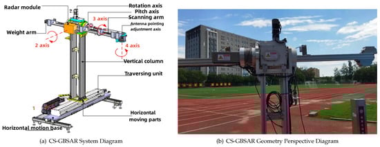
Figure 1.
Schematic diagram of CS-GBSAR.
The radar was deployed to monitor the Boyuan Building of North China University of Technology as the primary target, with the playground fence acting as a secondary target. The relative geometric configuration between the radar and targets is shown in Figure 1b. The system parameters of CS- GBSAR are shown in Table 1.

Table 1.
Parameters of CS-GBSAR system.
3. Method
In this section, we first introduce the basis of CA-CFAR detector and conventional DBSCAN. With this background information, we then introduce the detail of the proposed method, which includes two-step CFAR and modified DBSCAN.
3.1. CA-CFAR Detector
The two-parameter CFAR target detection algorithm is a well-established and widely used method in SAR image target detection. It is based on Gaussian background model for clutter, uses a sliding window to obtain mean and standard deviation for calculating the threshold [21,22,23]. Under the assumption that the clutter background follows a Gaussian distribution, the probability density function can be represented as:
The is the standard deviation, is the mean of the distribution, and the distribution function is:
The , then:
The standard probability density function of the normal distribution is:
Then, the false alarm probability can be derived [24]:
Then, the threshold is given as [25]:
where:
: is the standard deviation;
: is the mean of the distribution;
F(x): is the distribution function;
: is the false alarm probability;
: is the threshold.
The algorithm involves comparing each pixel in the image with a detection threshold . Pixels with values ≥ are identified as target points, while those with < are identified as clutter points. The probability distributions of target and background in SAR images can be observed from Figure 2, where the statistical distribution of target amplitude x is represented by p(x), and the noise and background amplitude distribution is represented by q(x). It is necessary to determine the optimal value of .
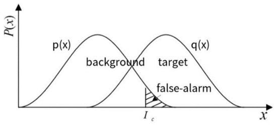
Figure 2.
Probability distribution of target and background.
False alarm probability corresponds to the probability of erroneously judging that an event has occurred due to interference caused by noise during target detection [26]. Radar signal detection often employs the Neyman–Pearson (NP) criterion, where the sufficient statistics are compared with adaptive thresholds through statistical hypothesis testing [27]. The aim of the NP criterion is to ensure optimal detection performance while maintaining a certain false alarm probability. In theory, the division of false alarms needs to integrate the distribution of background and target. In practice, the number of target units is usually less than that of background units, so the detection can adopt a suboptimal scheme, to determine whether the signal to be detected is the background.
The general process of CA-CFAR detection is as follows. It first utilizes the size of the detection window based on the size of the target to be detected. The classic hollow sliding window is shown in Figure 3, comprises the target area, protected area, and background area. The blue region represents the range of values, which is used to calculate the threshold . The white area represents the protected area, and the data in this area do not do any calculation. Then, compute the mean and variance based on a suitable number of pixel values around the target area selected by the sliding window. Then, using the given false alarm probability and the computed mean and variance, the threshold is determined. Finally, move the sliding window by point across the image, and at each position, the threshold is calculated and compared against the central pixel of the sliding window to determine whether it corresponds to a target point.
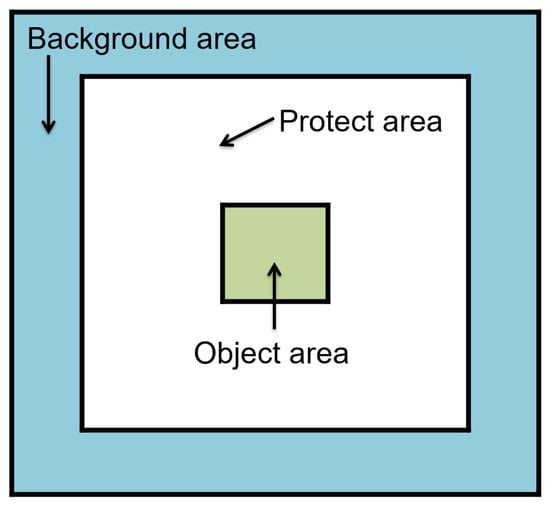
Figure 3.
Hollow sliding window.
3.2. Conventional DBSCAN
DBSCAN is a widely used density-based clustering algorithm that considers connectivity between samples based on their local density to determine the final clustering results. This involves extending the clusters by adding new connectable samples continuously. The algorithm employs two parameters: Eps and MinPts, which describe the sample distribution’s proximity in terms of neighborhood. Specifically, Eps is defined as the radius of the adjacent area surrounding a point, while MinPts stands for the minimum number of points required to form a cluster. The DBSCAN algorithm initially identifies a set of points satisfying at least MinPts within the Eps neighborhood as the starting cluster. Then, it gradually expands cluster by consistently including points that also satisfy the Eps and MinPts criteria until no more points qualify. A schematic depiction of the DBSCAN clustering principle is shown in Figure 4. The blue point represents that the pixels are clustered according to the clustering definition, while the red point does not conform to the clustering definition and is defined as the noise class.
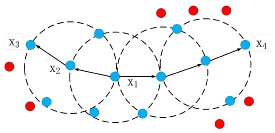
Figure 4.
DBSCAN clustering principle diagram.
However, the conventional DBSCAN algorithm has some drawbacks in processing 3D SAR data with uneven point cluster density and strong sidelobes. Firstly, selecting appropriate values for Eps and MinPts can be challenging since density changes in the cluster affect these parameters’ sensitivity. Because the template is spherical shape, if the Eps value is too large, it is hard to distinguish strong sidelobe point clusters diffused within the 3D point cloud, while a too-small Eps value might miss some free target point clusters. Secondly, even after performing the two-step CFAR algorithm to extract the initial 3D target point cloud, residual, randomly-distributed strong sidelobe points may still be present. Therefore, we propose a modified DBSCAN clustering algorithm that changes the clustering template with cylinder shape to suit the data’s own characteristics, so that the false alarm can be reduced. After clustering, a discrimination step is conducted to filter out strong sidelobe classes automatically based on target angle, shape, size, and position information present in the clustering results, leading to more accurate 3D point cloud extraction.
3.3. Proposed Method
Figure 5 shows the Flow chart of two-step CFAR CS-GBSAR 3D point cloud extraction method. The method includes the following basic steps. It first utilizes a maximum projection to obtain three-view images from 3D image data. Then, the first step CA-CFAR is applied to obtain the coarse masks of three-views. Then, the volume mask in original 3D image is obtained via inverse projection. This can remove strong sidelobes outside the potential target region and obtain potential target area data by intersecting it with the SAR 3D image. Then, the second step CA-CFAR is applied to potential target area data to obtain 3D point clouds. Finally, to further eliminate the residual strong sidelobes and output accurate 3D point clouds, the modified DBSCAN clustering algorithm is applied. The modified DBSCAN clusters with a cylindrical template to accommodate the data’s feature rather than the original spherical template, which can reduce false clustering. Then, it enables accurate extraction of the final 3D target point cloud.
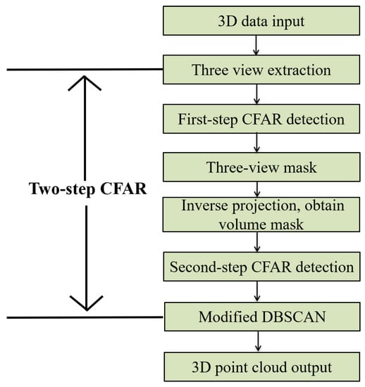
Figure 5.
Flow chart of two-step CFAR CS-GBSAR 3D point cloud extraction method.
While the classical two-parameter CFAR algorithm is capable of detecting target areas in 3D SAR images, it requires detect target layer by layer at different height. The strong sidelobes often hinder accurate detection of target points. Compared with the classical two-parameter CFAR layer by layer operation, this approach mitigates the impact of sidelobes and enables efficient extraction of 3D point clouds even when strong sidelobes are presented.
- Three view extractionTo begin with, we extract the three views of maximum value projection of three dimensions in the SAR 3D image and present the corresponding projection diagram in Figure 6. In each of the three views, the maximum value projection for each dimension ensures that all target points are preserved appropriately, thereby minimizing any potential loss of target points during subsequent steps of target point cloud extraction.
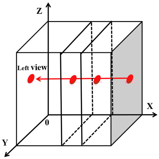 Figure 6. Three-view projection diagram.3D data are , the projection left-view , where is the direction vector of X axis; the projection front-view , where is the direction vector of Y axis; the projection top-view , where is the direction vector of the Z axis. As shown in Equation (7).
 - The first step CFARThe first step CFAR is to apply conventional CA-CFAR to the three-view image to obtain the three-view mask, as shown in Equation (8). They are left-view mask , front-view mask and top-view mask .where:: is left-view;: is front-view;: is top-view;: is left-view mask;: is front-view mask;: is top-view mask.By inverse projecting the three-view mask, the volume mask in the original 3D image is obtained, which is subsequently intersected with the SAR 3D image. This can remove strong sidelobes outside the potential target region and obtain potential target area data. Figure 7 depicts the process schematic. In Figure 6 and Figure 7, red, green, and blue correspond to the projections of pixels in the left view, the main view, and the top view, respectively. The purple sphere represents the intersection of projections in all data.
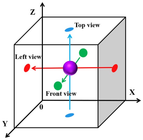 Figure 7. Three-view mask inverse projection schematic diagram.Three-view mask inverse projection process can obtain 3D mask . The corresponding derived formula is given as Equation (9).The 3D mask is then intersected with the 3D data to obtain the potential target area data . The corresponding derivation as shown in Equation (10).
 - The second step CFARThe second step CFAR is initiated to perform global two-parameter CFAR detection on the potential target area data . This produces the coarse 3D target point cloud represented by . The global CFAR is perform detection on the whole data rather than using the sliding window, because to the sidelobes are mostly eliminated in the previous step. In practice, it converts the whole extracted 3D data into a row vector, computing its mean and variance to determine the detection threshold , based on the constant false alarm probability. Subsequently, the central pixel of the sliding window is traversed in the potential target area data to detect more accurate target points. The derived formula is presented in Equation (11).
- The modified DBSCANIn response to the uneven cluster density of 3D data target points and their often linear structure in the vertical plane, we have proposed a modification to the conventional DBSCAN clustering algorithm. By imposing more constrained clustering conditions, we aim to obtain more accurate results for such cases. Specifically, we have introduced a change to the shape of the clustering metric from a sphere to a cylinder, as illustrated in Figure 8. This adjustment is particularly useful in addressing scenarios where there may be significant variation in point densities both within and between clusters. In Figure 8, the blue scatter points represent the pixels in the data. The blue sphere and the blue cylinder are the clustering constraint shape of the traditional DBSCAN method and the modified DBSCAN method, respectively.
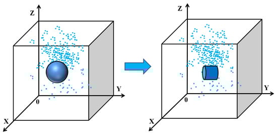 Figure 8. Clustering constraint shape diagram.The modified DBSCAN clustering algorithm utilizes three key parameters to describe the compactness of the point cloud distribution, namely, the neighborhood radius r in the x and z planes, the neighborhood distance h along the y-axis, and MinPts, which sets the minimum number of pixels required to form a cluster, which is the density threshold. These parameters should be tuned to achieve optimal clustering performance.Figure 9 is the diagram of a new clustering constraint for the cylindrical shape template. The red point represents any two points in the data. After derivation, Equation (12) provides a formula for determining the distance between different dimensions, while Equation (13) specifies the constraint conditions. It should be noted that these parameters are currently determined based on empirical experience, but future research may explore more optimal ways to identify suitable parameter configurations that can further enhance performance.
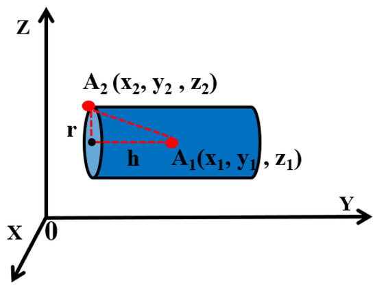 Figure 9. Clustering constraint condition diagram.where:: is the distance of x and z planes;: is the distance of height;r: is the cylindrical shape template radius;h: is the cylindrical shape template half the height.Our algorithm starts by randomly searching for pixels in the 3D target point cloud . For each identified pixel, the algorithm conducts a search within the cylindrical area, applying the previously defined constraints. Any cluster of pixels that contains more Minpts pixels as defined by our clustering conditions is marked and classified accordingly. Pixels that do not fit these criteria are labeled as noise. This process continues until all pixels are either classified into one or more clusters or classified as noise. As we note, the modified DBSCAN algorithm is represented by mDBSCAN in Equation (14). Through this method, we obtain the final clustering result , with a precise spatial distribution of points, which suit the 3D CS-GBSAR data.After the clustering process, we analyze the resulting data to filter out strong sidelobe classes based on target characteristics such as angle, shape, size and location. This filtering step improves the accuracy of our 3D point cloud extraction.
4. Experiment
In order to extract target information from the SAR data, we applied a maximum value projection method to generate three views of the data: a front view, top view, and left view, which are depicted in grayscale in Figure 10. In the front and top view, the reader can see bright points that correspond to the Boyuan Building and part of the playground fences. The other near circular-shaped line in the images are the sidelobe of the strong structures, which shows the phenomenon described previously. Figure 11 is the optical and top view images of the Boyuan Building. The blue box and red box labeled the playground’s fences and Bouyuan Building in optical and SAR image, respectively. The positions are matches as can be seen in the figure.
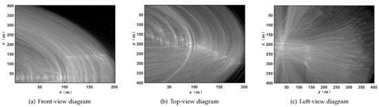
Figure 10.
Three-view diagram: (a) front-view diagram; (b) top-view diagram; (c) left-view diagram.
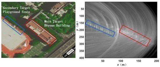
Figure 11.
The comparison between the front view and the optical vertical view of the Boyuan Building.
4.1. The First Step CFAR Detection Results
In the first step of CFAR target detection, we perform a maximum value projection to generate the front view, top view, and left view masks shown in Figure 12. During CFAR target detection, two critical factors directly impact the detection results: sliding window size and false alarm rate. Sliding windows are used to estimate the statistical characteristics of the target area while ensuring that the protected area prevents target leakage into the background area, which may affect calculation accuracy. Window size should match the target’s maximum size while utilizing an inner side length larger than the detection target. Background areas help estimate the statistical characteristics of the background, and its size can be selected according to experience based on the image resolution and object size [28].
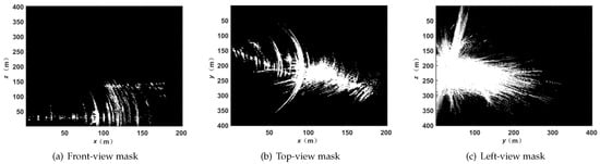
Figure 12.
Three-view masks: (a) front-mask; (b) top-mask; (c) left-mask.
The CS-GBSAR 3D image is in 201 × 401 × 401 size. The whole window size is 50 × 50, the size of the guard region is 30 × 30 and the pixel for detection is one pixel. The selection of false alarm probability affects the threshold directly, where targets will be missed if the threshold is too large and false alarms will increase if it is too small. For our SAR 3D image, we set the false alarm probability to 0.1, as recommended by empirical parameters. Using these masks, we obtain the volume mask in original 3D images via inverse projection. Then, we can obtain potential target area data by intersecting it with the SAR 3D image as depicted in Figure 13. The color of the point cloud in Figure 13 is changed according to the height, and different colors are used to distinguish the height.
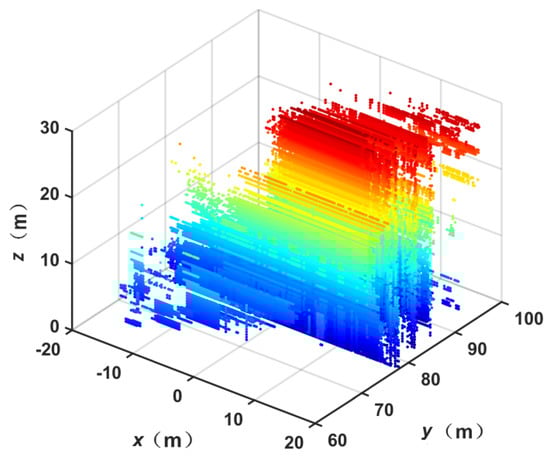
Figure 13.
Potential target point cloud image.
4.2. The Second Step CFAR Detection Results
In the second step of CFAR target detection, we utilize a global two-parameter CFAR algorithm to detect and generate more precise target points from the masks applied to the extracted data, which results in the initial extraction of 3D point clouds illustrated in Figure 14. To validate the results, Figure 15a–c presents a comparison between 3D point, optical image and LiDAR point clouds of the porch structure of the Boyuan Building. Meanwhile, the red boxes in all three subfigures mark the porch structure of the Boyuan Building.
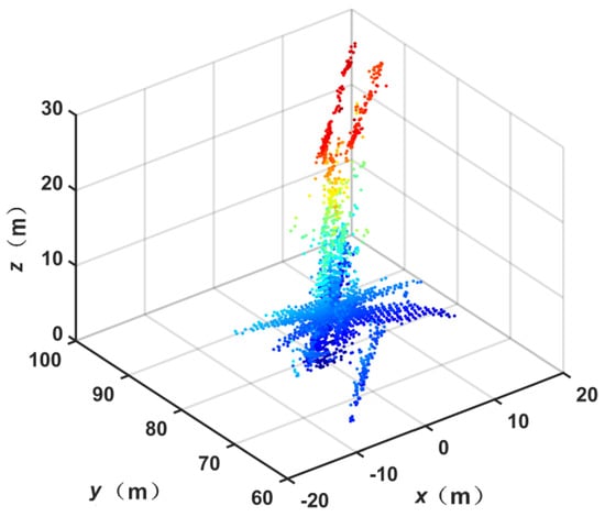
Figure 14.
3D target point cloud image.
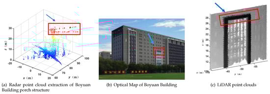
Figure 15.
Comparison between 3D point cloud and optical image and LiDAR point clouds of the porch structure of the Boyuan Building.
The laser detection and ranging (LiDAR) data in this paper are the external truth data. LiDAR is an active remote sensing technology that can generate accurate and high density 3D point cloud data. It can be used for generating high precision 3D models. Here, we use it to verify the accuracy of the method-extracted 3D structure of the porch structure of the Boyuan Building. In practice, we compare the length and height of the porch between LiDAR and the proposed method. The experimental truth value comparison table is shown in Table 2. We know from the experiment that the length of the porch structure in LiDAR point clouds is 10 m and the height is 28 m. The length of the porch structure in the detected 3D target point cloud is 11.67 m and the height is 28.4 m. The estimation difference in length and height are 1.67 m and 0.4 m, respectively, which is relatively close [29,30]. We can conclude both the radar and LiDAR point clouds match the length and height information of the two current porch structures of Boyuan Building as depicted in the optical image. The next step is to applied mDBSCAN to classify the points into cluster, so that the false detections can be reduced.
Table 2.
Comparison of proposed method and truth data.
To implement the mDBSCAN, three parameters, r, h, and MinPts, should be set. Based on empirical testing, the radius is set to 9 pixels, the cylinder height h is 3 pixels, and the density threshold MinPts is 8. The clustering results are illustrated in Figure 16. Each cluster is labeled with a unique color in the image. The number of all clusters is 22, we can see that the typical structures are all classified, and the noise points are less in the whole data. This figure demonstrates the successful separation of the target area from the remaining strong sidelobe point clusters, achieved through the modified DBSCAN clustering algorithm.
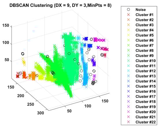
Figure 16.
Modified DBSCAN method clustering results with strong sidelobes.
In Figure 17, we observe distinct 3D spatial distribution characteristics between the target class and the strong sidelobe class in angle, shape, size, and position differences. The biggest cluster is the strong scatter and its sidelobe, which can be seen as a cross structure. The reason for its existence is a staircase from the trihedral-shaped structure as shown in Figure 17a’s optical image. Its presence influences the quality of the points extraction results. Based on the angle, shape, size, and position differences, this strong scatter and sidelobe can be removed effectively, and the final extraction results are illustrated in Figure 17b. Then, the precise extraction of the point cloud from the 3D SAR image is achieved.
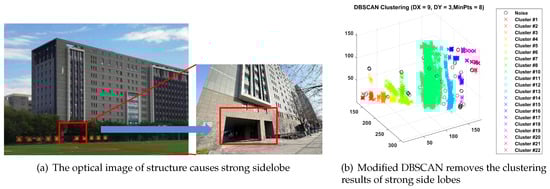
Figure 17.
The clustering results of removing sidelobes are compared with the optical images.
5. Discussion
As introduced in the introduction, to the best of our knowledge, there is no relevant research on the 3D point cloud extraction method for CS-GBSAR. However, research on the CA-CFAR method for 2D SAR image target detection has been deeply studied and widely applied, which can be used as the candidate for solving the problem. For the problem of multi-target detection, Cui et al. [31] proposed a CFAR target detection method based on iterative filtering in 2011, which avoids the interference of multiple targets. Chen Xiang et al. [32] proposed a ship detection algorithm based on CFAR cascade in SAR images in 2012. It can solve the problem of multi-target and clutter edge at the same time. Song et al. [33] proposed an automatic region screening SAR target detection algorithm in 2016. It has stable detection performance and false alarm suppression ability. Huang et al. [34] proposed a semantic CFAR target detection algorithm. Compared with the traditional CFAR using only intensity information, it can remove a large number of strong clutter false alarms without shadows. To dispose of the effect of the target pixels near the PUT (Pixel Under Test), Pappas et al. [35] proposed a superpixel-level CFAR detection method in 2018. It utilizes superpixels instead of rectangular sliding windows to define CFAR guard areas and clutter. The objective is to enhance target exclusion from outliers while reducing false detections. Ai et al. [36] proposed the BTSR-CFAR (Robust Bilateral-Trimmed-Statistics-CFAR) detector in 2021, it eliminates the capture effect arising in conventional CFAR detectors. In 2023, Li Yu et al. [37] proposed the Multi-source Fusion CFAR Detection Method Based on the Contrast of Sliding Window, the proposed algorithm fully exploits the distribution characteristics of target energy in multi-station fusion images and provides an effective way for multi-source fusion target enhancement detection.
The above-mentioned CFAR methods are all based on on two-dimensional SAR images, which cannot be applied to CS-GBSAR. As will be shown in the following section, the conventional layer by layer method cannot accurately extract the 3D point cloud. The strong sidelobe will degrade the extraction performance. The proposed two-step CFAR can avoid such influence, which demonstrates the necessity of proposed method.
Section 5.1 is the comparison of the proposed method with the conventional method. Section 5.2 gives a summary of the proposed method and the future research directions.
5.1. Comparison with the Results of Traditional Methods
This section presents the method comparison experiment to demonstrate the necessity of the proposed method, i.e., the classical two-parameter CFAR layer-by-layer detection algorithm and the two-step CFAR detection algorithm. Subsequently, both the traditional DBSCAN clustering algorithm and the modified DBSCAN clustering algorithm were applied to extract the point cloud and suppress false alarms.
The comparison results of the resulting 3D initial point cloud views are depicted in Figure 18. Figure 18a is the 3D initial point cloud extracted by two-parameter CFAR layer-by-layer detection, and (b) is the 3D initial point cloud extracted by two-step CFAR detection. The image obtained via the two-step CFAR algorithm preserves the target area with significantly reduced sidelobes, resulting in a clearer extraction. While the conventional method has more clutters remain in each layer. The parameters of the conventional method are optimized to reach the best performance.
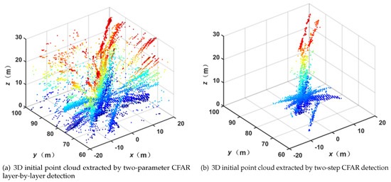
Figure 18.
Comparison results of 3D target initial point cloud view results.
To further show the difference, the three-view of the initial extraction result of the 3D target point cloud is shown in Figure 19. Figure 19a–c are the three-view projection of the initial extraction point cloud after the classical two-parameter CFAR target detection algorithm is detected layer by layer. Figure 19d,e are generated by the two-step CFAR algorithm. The main target area is labeled by a red box, and the secondary target is labeled by a blue box. The main target area is the porch structure of the Boyuan Building of North China University of Technology, and the secondary target is the playground fence. Through a comparison of results obtained using the two-parameter CFAR algorithm and the two-step CFAR algorithm, it becomes evident that the classical two-parameter CFAR algorithm produces an abundance of false alarms, which fails to accurately distinguish the target area from the existing detection results, while the proposed method is clearer. Hence, the two-step CFAR algorithm proves more effective for SAR 3D image target detection with complex backgrounds, making it ideal for the initial extraction of 3D imaging point clouds.
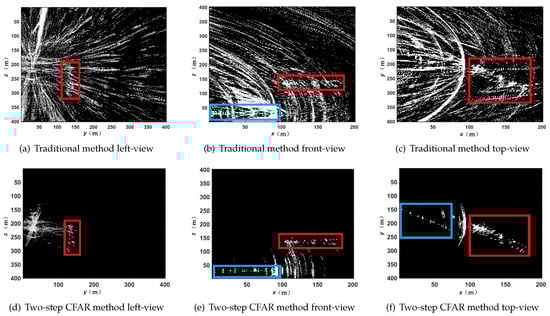
Figure 19.
Comparison of 3D target initial point cloud three view projection results.
Figure 20 illustrates the comparison results of 3D point cloud clustering using two different methods: (a) is the traditional DBSCAN clustering result; (b) is the modified DBSCAN clustering result; and (c,d) are two method results from removing the strong sidelobe. Although both the methods classify targets and strong sidelobes into separate clusters, the traditional DBSCAN clustering result contains more noise points, which are wrongly classified. In such condition, it is impossible to accurately cluster and distinguish the target class and the strong sidelobe class, and the false alarm suppression effect is poor. The conventional DBSCAN clustering algorithm noise class contains 1225 points, while the modified DBSCAN clustering algorithm noise class contains 56 points. The comparison experiment shows that the proposed method can reduce 95.4% false clustered points and remove the strong traces, which shows the better performance of the proposed method. The modified DBSCAN algorithm has less noise points in the clustering results. It can distinguish the target from the residual strong sidelobes while maintaining a certain noise reduction ability. It restores the positioning information of each point cluster greatly, making the point cloud extraction results more accurate and the target clearer.
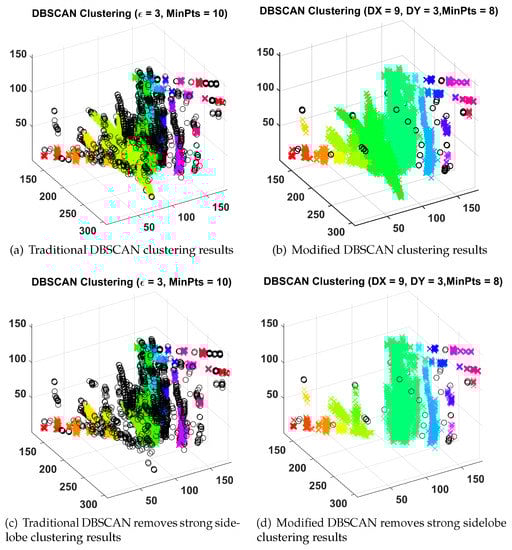
Figure 20.
Comparison results of 3D point cloud clustering.
In a similar way, the three-view comparison results are demonstrated through 3D point cloud clustering as in Figure 21. Figure 21a–e are three view of point cloud results generated by conventional DBSCAN and a modified DBSCAN algorithm, respectively. The traditional method left view, front view, and top view consecutively illustrate that traditional DBSCAN clustering outcomes contain a lot of noise, mistakenly classifying more positioning points as noise. The modified DBSCAN algorithm correctly identifies strong sidelobe point clusters diffused in the whole data and separates them from the target and strong side lobe point clusters. The modified DBSCAN algorithm reduces noise significantly and extracts more accurate target spatial distribution information. Hence, precise extraction of a 3D SAR image target point cloud is achieved.
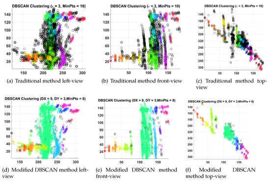
Figure 21.
Comparison of 3D target point cloud clustering three view projection results.
5.2. Summary of Proposed Method
Figure 22 summarize the proposed method. The left column is the main steps of proposed method. The right column is the summary. The three-view extraction is to ensure all potential target points are properly reserved, by maximum projection at three views. Then, the first step CFAR is to extract the coarse point cloud in three-view images. The next two steps can remove the sidelobes in the spatial position, which greatly reduces the 3D spatial influence of the strong sidelobes. However, parameters need to be adjusted empirically. Then, the second step CFAR is to performed on the potential target area to obtain the accurate point cloud in 3D data, which can be used as the input for clustering. The last step is modified DBSCAN. It uses cylindrical template to classify the clusters with high precision, it reduces the false clusters more than the original DBSCAN. However, due to the change in shape, the parameters for tuning are increased, which currently need to be adjusted by experimental testing to obtain better results. In the future, we will collect a large number of new data in different scenarios to test the method and continue to improve it to handle all possible scenarios.
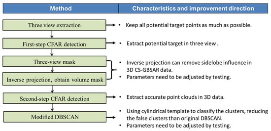
Figure 22.
Summary of proposed method.
6. Conclusions
The Circular Scanning Ground-Based Synthetic Aperture Radar (CS-GBSAR ) has the unique advantage of 3D imaging due to the nonlinear observation geometry. However, such nonlinear observation geometry causes strong sidelobes in SAR image, which make it a difficult task to extract point cloud data. The CA-CFAR algorithm can extract 3D point cloud data layer-by-layer at different heights, which is time consuming and is easily influenced by strong sidelobes to obtain inaccurate results. This paper proposes a new two-step CFAR-based 3D point cloud extraction method for CS-GBSAR, which can extract accurate 3D point cloud data under the influence of strong sidelobes. It first utilizes maximum projection to obtain three-view images from 3D image data. Then, the first step CA-CFAR is applied to obtain the coarse masks of three-views. Then, the volume mask in the original 3D image is obtained via inverse projection. This can remove strong sidelobes outside the potential target region and obtain potential target area data by intersecting it with the SAR 3D image. Then, the second step CA-CFAR is applied to potential target area data to obtain coarse 3D point clouds. Finally, to further eliminate the residual strong sidelobes and output accurate 3D point clouds, the modified DBSCAN clustering algorithm is applied. The modified DBSCAN clusters with a cylindrical template to accommodate the data’s features rather than the original spherical template, which can reduce false clustering. The acquired real data using the North China University of Technology (NCUT)-developed CS-GBSAR system validates the proposed method. The comparison with the conventional method shows that the proposed method has better performance.
In the future, we will conduct a quantitative analysis on setting the parameters of the proposed method, and study the data-driven CFAR to further improve the proposed method to suit the different data’s statistical distribution. Additionally, we will collect a large amount of new data in different scenarios to test the method and continue to improve it to handle all possible scenarios.
Author Contributions
W.S. and J.Z. performed the experiments and method. W.S. and J.Z. wrote the manuscript. Y.W., J.S., Y.L. (Yang Li), Y.L. (Yun Lin) and W.J. gave valuable advice on manuscript writing. All authors have read and agreed to the published version of the manuscript.
Funding
This work was supported by the National Natural Science Foundation of China under Grant 62201011, 62131001 and the R&D Program of the Beijing Municipal Education Commission grant KM202210009004 and North China University of Technology Research funds 110051360023XN224-8, 110051360023XN211.
Informed Consent Statement
Informed consent was obtained from all subjects involved in the study.
Data Availability Statement
Not applicable.
Conflicts of Interest
The authors declare no conflict of interest.
References
- Lin, Y.; Song, Y.; Wang, Y.; Li, Y. The large field of view fast imaging algorithm for arc synthetic aperture radar. J. Signal Process. 2019, 35, 499–506. [Google Scholar]
- Zhang, J.; Wu, J.; Wang, X. Application of ground based synthetic aperture radar in monitoring and early warning of mining area slope. Geotech. Investig. Surv. 2021, 49, 59–62. [Google Scholar]
- Wang, Y.; Song, Y.; Hong, W.; Zhang, Y.; Lin, Y.; Li, Y.; Bai, Z.; Zhang, Q.; Lv, S.; Liu, H. Ground-based differential interferometry SAR: A review. IEEE Geosci. Remote Sens. Mag. 2020, 8, 43–70. [Google Scholar] [CrossRef]
- Lee, H.; Ji, Y.; Han, H. Experiments on a Ground-Based Tomographic Synthetic Aperture Radar. Remote Sens. 2016, 8, 667. [Google Scholar] [CrossRef]
- Tebaldini, S. Single and multipolarimetric SAR tomography of forested areas: A parametric approach. IEEE Trans. Geosci. Remote Sens. 2010, 48, 2375–2387. [Google Scholar] [CrossRef]
- Aguilera, E.; Nannini, M.; Reigber, A. A data-adaptive compressed sensing approach to polarimetric SAR tomography of forested areas. IEEE Geosci. Remote Sens. Lett. 2013, 10, 543–547. [Google Scholar] [CrossRef]
- Zhu, X.X.; Bamler, R. Very high resolution spaceborne SAR tomography in urban environment. IEEE Trans. Geosci. Remote Sens. 2010, 48, 4296–4308. [Google Scholar] [CrossRef]
- Zhu, X.X.; Bamler, R. Demonstration of super-resolution for tomographic SAR imaging in urban environment. IEEE Trans. Geosci. Remote Sens. 2012, 50, 3150–3157. [Google Scholar] [CrossRef]
- Wang, Y.; Zhang, Q.; Lin, Y.; Zhao, Z.; Li, Y. Multi-Phase-Center Sidelobe Suppression Method for Circular GBSAR Based on Sparse Spectrum. IEEE Access 2020, 8, 133802–133816. [Google Scholar] [CrossRef]
- Zhang, Y.; Zhang, Q.; Wang, Y.; Lin, Y.; Li, Y.; Bai, Z.; Li, F. An approach to wide-field imaging of linear rail ground-based SAR in high squint multi-angle mode. J. Syst. Eng. Electron. 2020, 31, 722–733. [Google Scholar]
- Wang, Y.; He, Z.; Zhan, X.; Fu, Y.; Zhou, L. Three-dimensional sparse SAR imaging with generalized lq regularization. J. Remote Sens. 2022, 14, 288. [Google Scholar] [CrossRef]
- Feng, S.; Lin, Y.; Wang, Y.; Yang, Y.; Shen, W.; Teng, F.; Hong, W. DEM Generation With a Scale Factor Using Multi-Aspect SAR Imagery Applying Radargrammetry. Remote Sens. 2020, 12, 556. [Google Scholar] [CrossRef]
- Zhang, L.; Zhang, J.; Zhang, X.; Lang, H. Task distribution balancing for parallel two-parameter CFAR ship detection. J. Remote Sens. 2016, 20, 344–351. [Google Scholar]
- Du, L.; Wang, Z.; Wang, Y.; Wei, D.; Li, L. Survey of research progress on target detection and discrimination of single-channel SAR images for complex scenes. J. Radars. 2020, 9, 34–54. [Google Scholar]
- Ai, J.; Yang, X.; Song, J.; Dong, Z.; Jia, L.; Zhou, F. An adaptively truncated clutter-statistics-based two-parameter CFAR detector in SAR imagery. IEEE J. Ocean. Eng. 2018, 43, 269–279. [Google Scholar] [CrossRef]
- Zhu, Z.; Zhou, N.; He, S. Identification of offshore fixed facilities and dynamic ships based on sentinel-1A. Remote Sens. Inform. 2022, 37, 77–86. [Google Scholar]
- Ester, M.; Kriegel, H.P.; Sander, J.; Xu, X. A Density-based Algorithm for Discovering Clusters in Large Spatial Databases with Noise. In Proceedings of the Second International Conference on Knowledge Discovery and Data Mining, Portland, OR, USA, 2–4 August 1996; pp. 226–231. [Google Scholar]
- Bushra, A.A.; Yi, G. Comparative Analysis Review of Pioneering DBSCAN and Successive Density-based Clustering Algorithms. IEEE Access 2021, 9, 87918–87935. [Google Scholar] [CrossRef]
- Schubert, E.; Sander, J.; Ester, M.; Kriegel, H.P.; Xu, X. DBSCAN revisited, revisited: Why and how you should (still) use DBSCAN. ACM Trans. Database Syst. 2017, 42, 1–21. [Google Scholar] [CrossRef]
- Li, S.S. An Improved DBSCAN Algorithm Based on the Neighbor Similarity and Fast Nearest Neighbor Query. IEEE Access 2020, 8, 47468–47476. [Google Scholar] [CrossRef]
- Li, L. Study of SAR Target Detection and Recognition with Feature Fusion. Ph.D. Dissertation, Xidian University, Xi’an, China, 2021. [Google Scholar]
- Banerjee, A.; Burlina, P.; Chellappa, R. Adaptive target detection in foliage-penetrating SAR images using alpha-stable models. IEEE Trans. Image Process. 1999, 8, 1823–1831. [Google Scholar] [CrossRef]
- Zhang, L.; Zhang, Z.; Lu, S.; Xiang, D.; Su, Y. Fast Superpixel-Based Non-Window CFAR Ship Detector for SAR Imagery. Remote Sens. 2022, 14, 2092. [Google Scholar] [CrossRef]
- Wang, C.; Liao, M.; Li, X. Ship Detection in SAR Image Based on the Alpha-stable Distribution. Sensors 2008, 8, 4948–4960. [Google Scholar] [CrossRef] [PubMed]
- Gao, G.; Liu, L.; Zhao, L.; Shi, G.; Kuang, G. An adaptive and fast CFAR algorithm based on automatic censoring for target detection in high-resolution SAR images. IEEE Trans. Geosci. Remote Sens. 2008, 47, 1685–1697. [Google Scholar] [CrossRef]
- Li, T.; Liu, Z.; Xie, R.; Ran, L. An Improved Superpixel-Level CFAR Detection Method for Ship Targets in High-Resolution SAR Images. IEEE J. Sel. Top. Appl. Earth Obs. Remote Sens. 2018, 11, 184–194. [Google Scholar] [CrossRef]
- Zhang, L.; Ding, G.; Wu, Q.; Zhu, H. Spectrum Sensing Under Spectrum Misuse Behaviors: A Multi-Hypothesis Test Perspective. IEEE Trans. Inf. Forensics Secur. 2018, 13, 993–1007. [Google Scholar] [CrossRef]
- Zhang, F.; Zhou, H.; Lei, L. An CFAR detection algorithm based on local fractal dimension. Signal Process. 2012, 28, 7. [Google Scholar]
- Altuntas, C. Review of Scanning and Pixel Array-Based LiDAR Point-Cloud Measurement Techniques to Capture 3D Shape or Motion. Appl. Sci. 2023, 13, 6488. [Google Scholar] [CrossRef]
- Xu, J.; Yao, C.; Ma, H.; Qian, C.; Wang, J. Automatic Point Cloud Colorization of Ground-Based LiDAR Data Using Video Imagery without Position and Orientation System. Remote Sens. 2023, 15, 2658. [Google Scholar] [CrossRef]
- Cui, Y.; Zhou, G.; Yang, J.; Yamaguchi, Y. On the Iterative Censoring for Target Detection in SAR Images. IEEE Geosci. Remote Sens. Lett. 2011, 8, 5. [Google Scholar] [CrossRef]
- Chen, X.; Sun, J.; Yin, K.; Yu, J. An algorithm of ship target detection in SAR images based on cascaded CFAR. Modern Radar. 2012, 34, 50–54, 58. [Google Scholar]
- Song, W.; Wang, Y.; Liu, H. An automatic block-to-block censoring target detector for high resolution SAR image. J. Electron. Inf. Technol. 2016, 38, 1017–1025. [Google Scholar]
- Huang, Y.; Liu, F. Detecting cars in VHR SAR images via semantic CFAR algorithm. IEEE Geosci. Remote Sens. Lett. 2016, 13, 801–805. [Google Scholar] [CrossRef]
- Pappas, O.; Achim, A.; Bull, D. Superpixel-Level CFAR Detectors for Ship Detection in SAR Imagery. IEEE Geosci. Remote Sens. Lett. 2018, 15, 1397–1401. [Google Scholar] [CrossRef]
- Ai, J.; Mao, Y.; Luo, Q.; Xing, M.; Jiang, K.; Jia, L.; Yang, X. Robust CFAR Ship Detector Based on Bilateral-Trimmed-Statistics of Complex Ocean Scenes in SAR Imagery: A Closed-Form Solution. IEEE Trans. Aerosp. Electron. Syst. 2021, 57, 1872–1890. [Google Scholar] [CrossRef]
- Li, Y.; Zhang, S.; Mao, C.; Yan, H.; Li, C.; Duan, C. Multi-source Fusion CFAR Detection Method Based on the Contrast of Sliding Window. Modern Radar. 2023, 45, 25–30. [Google Scholar]
Disclaimer/Publisher’s Note: The statements, opinions and data contained in all publications are solely those of the individual author(s) and contributor(s) and not of MDPI and/or the editor(s). MDPI and/or the editor(s) disclaim responsibility for any injury to people or property resulting from any ideas, methods, instructions or products referred to in the content. |
© 2023 by the authors. Licensee MDPI, Basel, Switzerland. This article is an open access article distributed under the terms and conditions of the Creative Commons Attribution (CC BY) license (https://creativecommons.org/licenses/by/4.0/).