MEC Server Sleep Strategy for Energy Efficient Operation of an MEC System

Abstract

Optimizing the energy consumption of an MEC (Multi-Access Edge Computing) system is a crucial challenge for operation cost reduction and environmental conservation. In this paper, we address an MECS (MEC Server) sleep control problem that aims to reduce the energy consumption of the system while providing users with a reasonable service delay by adjusting the number of active MECSs according to the load imposed on the system. To tackle the problem, we identify two crucial issues that influence the design of an effective sleep control technique and propose methods to address each of these issues. The first issue is accurately predicting the system load. Changes in system load are spatio-temporally correlated among MECSs. By leveraging such correlation information with STGCN (Spatio-Temporal Graph Convolutional Network), we enhance the prediction accuracy of task arrival rates for each MECS. The second issue is rapidly selecting MECSs to sleep when the load distribution over an MEC system is given. The problem of choosing sleep MECS is a combinatorial optimization problem with high time complexity. To address the issue, we employ a genetic algorithm and quickly determine the optimal sleep MECS with the predicted load information for each MECS. Through simulation studies, we verify that compared to the LSTM (Long Short-Term Memory)-based method, our method increases the energy efficiency of an MEC system while providing a compatible service delay.

1. Introduction

The increasing prevalence of high-speed wireless networks, smart mobile devices, and digital services has led to a connected and data-centric society, driving innovation and economic growth across various industries. This digital transformation poses complex challenges such as low-latency data processing, efficient bandwidth utilization, and improved service quality. In response, Multi-Access Edge Computing (MEC) systems have garnered significant attention. MEC systems deploy numerous low-capacity MEC servers (MECSs) at the network edge, utilizing computing and storage resources for low-latency services. This is crucial for applications such as autonomous vehicles, augmented reality, real-time gaming, and healthcare. MEC systems efficiently manage network bandwidth and reduce congestion by processing data at the edge before transmitting it to central data centers. However, the benefit of an MEC system does not come without costs. With the expansion of the service area in MEC systems, there is an associated increase in the required number of MECSs. This escalation in the number of MECS contributes to a higher energy consumption, resulting in an augmented operational expenditure for the MEC system. In addition, networks and data centers are expected to account for 59.8% of the CO₂ emissions in the information and communications technology sector by 2030 [1]. Therefore, it is essential to increase the energy efficiency of an MEC system to reduce the operational cost and tackle the environmental conservation problem.

An MECS undertakes the reception, processing, and subsequent transmission of results for tasks offloaded from users. Consequently, the energy consumed within an MEC system is categorized into the communication energy and computing energy of MECS. In the task-offloading process, a user device incurs transmission power consumption. Given the typically small size of service results, the downlink transmission power of an MECS is often assumed to be negligible. However, if an MECS cannot handle a service for processing the requested task, task migration to a cloud server or another MECS becomes necessary, constituting a significant portion of the communication energy within an MECS. To mitigate the energy impact of task migration, various service caching methods have been proposed [2,3,4]. Given the potential minimization of communication energy using appropriate service caching methods, this paper concentrates on addressing the computing energy consumption issue. Since an MEC system involves complex interactions among diverse elements, a multitude of approaches have been proposed to mitigate computing energy consumption across various facets of MEC systems. For instance, the energy consumed in an MEC system can be reduced via an optimal offloading decision [5], resource management [6], network selection [7], and dynamic voltage and frequency scaling [8]. These methodologies presuppose the active mode for all MECSs within the system, overlooking the temporal and spatial variations in tasks offloaded to each MECS. Generally, the workload imposed on an MEC system is unevenly distributed across MECSs. Thus, when the total system load is below the combined capacity of all MECSs, some MECSs may remain lightly loaded or idle. However, an MECS consumes a substantial amount of energy even in the idle state [9]. To address this, minimizing the total energy consumption of an MEC system involves placing unnecessary MECSs into a sleep state. However, since only active MECSs process loads in an MEC system, the service delay increases with the number of MECSs in the sleep state. Consequently, determining the operation mode of each MECS based on workload distribution becomes crucial for effectively reducing energy consumption while maintaining a reasonable service quality.

Various MECS sleep control methods have been proposed to strike a delicate balance between two conflicting performance metrics: the amount of energy consumed and the service latency delivered by an MEC system. Threshold methods [10,11], commonly employed in determining the operational mode of an MECS, involve transitioning an MECS into sleep mode when its load falls below a predefined threshold. This approach, wherein each MECS independently decides based on its own workload, is straightforward to implement. However, the uneven distribution of the load across MECSs at each time step prompts the exploration of comprehensive load distribution considerations to optimize system-wide energy efficiency. Addressing this, cooperative sleep decision methods have been proposed [9,12], where MECSs form clusters, exchange status information, and make sleep decisions, considering the status of other MECSs in the same cluster. Despite the potential enhancement in energy efficiency, such cooperative methods introduce additional signaling overhead, and when MECS decisions differ, an iterative consensus process ensues, potentially leading to delayed decision making. To tackle these challenges, deep learning models have been used [13,14]. These approaches leverage the current load information of MEC at a specific time point to predict the load of each MECS in the subsequent time step. Subsequently, decisions are made regarding which MECS should sleep based on these predictions. To forecast the MECS load, these techniques often model the MECS load as a time-series sequence and predominantly employ the LSTM (Long Short Term Memory) model as it is suitable for time-series data prediction. In this approach, the accuracy of the determined set of sleep MECS based on predicted values depends on the precision of load prediction for each MECS. Therefore, the optimization of the sleep MECS decision problem can be reframed as a precise workload prediction problem.

However, since LSTM was originally developed for the prediction of Euclidean data, its performance may degrade when applied to non-Euclidean data with graph structures like MEC systems. Therefore, in this paper, we improve the previous method based on the LSTM predictor in two major aspects. Firstly, we improve the accuracy of the predicted task arrival rate. The task arrival rate to an MECS varies in time and space. However, LSTM exploits only the correlation in the time domain, neglecting the valuable correlation information in the space domain. We enhance the accuracy of task arrival rate prediction by using STGCN (Spatio-Temporal Graph Convolution Network) [15]. STGCN extends the convolution operations commonly used in graph neural networks to both spatial and temporal dimensions to effectively capture information between neighboring nodes and detects temporal changes, providing enhanced capabilities in modeling spatio-temporal data. Secondly, we reduce the prediction delay. Since LSTM has a recurrent architecture, it processes inputs sequentially. Therefore, the methods based on LSTM are slow in producing predicted values. On the contrary, since we use the STGCN model that can process inputs in parallel, we can reduce the time needed to produce predicted values. We can summarize our contributions as follows.

• We propose a framework for the MECS sleep decision by using STGCN. We define an input graph for this framework and enhance the prediction accuracy for the workload distribution in an MEC system by utilizing not only the workload correlations in each MECS in the time domain, but also the relationships among MECSs in the space domain.
• Despite the availability of the workload distribution information, determining the operational modes of individual MECS poses a computationally challenging combinatorial optimization problem. To address this, we utilize a genetic algorithm (GA) to fast compute the optimal operation mode for each MECS at the start of each time slot, taking into account both energy consumption and service latency factors for all MECSs in the system.
• Comprehensive simulation studies show that our approach is better than the conventional LSTM-based method in terms of both energy efficiency and the time required for determining sleep MECSs.

The organization of this paper is as follows. We present related works in Section 2. In Section 3, we describe the system model and cast the sleep control problem. We describe our MECS sleep decision method in Section 4. In Section 5, we verify the proposed method by evaluating its performance via extensive simulation studies. We conclude the paper with future research directions in Section 6.

2. Related Works

2.1. Preliminary: Graph Neural Networks

Graph neural network (GNN) is a term used to represent the artificial neural networks designed to process data represented as graphs. The key tasks of GNN include node level tasks, edge level tasks, and graph-level tasks. In the node level tasks, GNN learns the features of individual graph nodes by considering their attributes and connectivity. The learned features can be used for new node classification. For the edge level tasks, a GNN embeds edge features and uses them to predict possible links and weights indicating the strength of each connection in a graph. Graph-level tasks involve predicting or classifying features of the entire graph. For example, it can be used to identify communities within the entire social graph and create new protein molecules. In general, a computation module in a GNN is composed of a message function, aggregation function, update function, and readout function. Depending on the configuration of these functions in the computational module, various GNNs can be built [16,17]. In [18], according to the primary objectives and architectural differences of various GNNs, the authors categorize a set of GNNs into RecGNN (Recurrent GNN), ConvGNN (Convolutional GNN), GAE (Graph AutoEncoder), and STGNN (Spatial-Temporal GNN). RecGNNs aim to learn node representations via recurrent structures, introducing the concept of message passing, where nodes exchange information with neighboring nodes until reaching a stable state. This message passing idea is adopted by ConvGNNs. ConvGNNs generalize the convolution from Euclidean data space to non-Euclidean data space, providing a foundation for constructing other complex GNNs. GAEs are an unsupervised learning model that encodes nodes or graphs into a latent vector space and generates new graphs using embedded graph information. STGNNs focus on learning hidden patterns of graphs that change spatio-temporally, considering the spatio-temporal correlations of graph information simultaneously. We summarize the GNN categories in Table 1. For a further review of graph neural networks, we refer the readers to [16,17,18] and the references therein.

Table 1. Categories of GNNs.

Category	Main Goal	Architectural Property
RecGNNs (Recurrent GNNs)	Learn node representation	Recurrent architecture and message passing
ConvGNNs (Convolutional GNNs)	Node/graph classification	Extend convolution to non-Euclidean data space
GAEs (Graph AutoEncoders)	Node/graph encoding, graph generation	Autoencoder using graph convolution
STGNNs (Spatial-Temporal GNNs)	Learn latent spatio-temporal pattern in a graph	Graph convolution, CNN, RNN

In this paper, we aim to predict the workload of each MECS by considering the relationship among the MECSs both in the time domain and the space domain. An MEC system consists of MECSs, which are deployed at the network edge. In an MEC system, control messages are exchanged between geographically adjacent MECSs for the efficient operation of the system. Therefore, by considering MECSs as nodes and the geographical relationships between adjacent MECSs as links, the MEC system can be modeled as a graph. Since an MECS serves tasks offloaded by users, the load of an MECS is determined by the number of users and their task-offloading patterns within the MECS service area. Additionally, the locations of users change over time, and the mobility of users is physically constrained within a certain distance over a specified period. Consequently, changes in the user set for each MECS over time impact the user set of neighboring MECSs, influencing the load of each MECS based on the load of neighboring MECSs. In other words, the load of each MECS is closely related with the load of its neighboring MECSs over time and space. Due to its ability to consider spatio-temporal correlations among the related entities, STGNN is being applied to various applications. For example, in [19], STGNN is used for road traffic prediction by exploiting complex spatio-temporal correlation of traffic flow. In [20], STGNN is used for skeleton-based human action cognition by making use of the skeleton topology information. Motivated by these research trends and the characteristics of the load distribution in an MEC system, we chose STGCN which belongs to the STGNN category for predicting the load distribution in an MEC system. Specifically, we extract node features by representing the spatio-temporal relationships among the loads of each MECS by adopting STGCN. Then, by using the extracted node features, we predict the load across each MECS. Subsequently, we utilize this information to determine the optimal selection of MECSs to sleep by using a genetic algorithm.

2.2. Energy Saving in an MEC System

In line with the energy-saving objectives, studies pertaining to energy efficiency in an MEC system can be classified into two primary groups. The first group is dedicated to diminishing the energy consumption in end devices, while the second group is centered around addressing the energy consumption within an MEC system. User devices have the potential to conserve energy through the offloading of computing tasks to an MEC system. However, the task-offloading process itself entails the consumption of transmission power by the user device. Furthermore, task offloading can introduce an increase in task completion delay since the processed results are delivered to the user device after the task is sent to and processed within an MEC system. Consequently, various task-offloading decision methods are proposed to minimize the energy consumption of a user device. These methods take into account factors such as computing power, transmission power, and task completion delay [21,22,23].

To minimize the energy consumption of an MEC system while providing a reasonable quality of service to end users, various resource management methods have been proposed [24]. Load-balancing methods among MECSs are proposed in [25,26] to increase the resource efficiency of an MEC system while reducing the system cost. The authors in [27,28] propose optimal computation resource allocation methods to reduce the energy consumption of an MECS while ensuring the service delay requirement in each MECS. Content caching methods are proposed in [29,30] to accommodate the massive computation demands from users in an energy-efficient manner. Service placement schemes are proposed to reduce both service completion time and energy consumption by placing the services requested by users to their serving MECS [31,32].

However, these studies are primarily focused on designing the intended functionalities in an energy-efficient manner. In other words, they assume all MECSs are always in an active mode. However, servers consume a considerable amount of energy even in the idle state. Therefore, if a majority of MECS are underloaded, a potential strategy for decreasing the overall energy consumption of an MEC system is to activate only a subset of MECSs to handle tasks while putting the remaining MECSs in a sleep state.

2.3. Sleep Control Methods

Various methods have been proposed to increase the energy efficiency of an MEC system by controlling the working mode of the MECSs. These methods can be broadly categorized into distributed methods and centralized methods. Distributed methods use meta-heuristic optimizations, a bio-inspired method, and game theory. Centralized methods use the Lyapunov optimization framework, machine learning, and deep learning methods.

The authors in [33] use the particle swarm optimization (PSO) algorithm to control the operation mode of MECSs. They formulate the MECS sleep control problem as a two-dimensional optimization problem. Then, they propose a user connection matrix-based AP sleeping method by using PSO. In the work presented in [12], a bio-inspired method for controlling the sleep states of MECSs is proposed, drawing inspiration from the inter-cell signaling mechanism. At the end of each time slot, each MECS engages in periodic load information exchanges with its neighboring MECSs. Through a distributed process involving the comparison of relative load levels with those of neighboring MECSs, each MECS autonomously determines its operational mode. In the study presented in [34], the authors employ the minority game theory to decide the operational mode of an MECS. They tackle the distributed computation offloading problem, taking into account the determination of the MECS operation mode. The minority game is utilized to seek an equilibrium state that optimally balances the latency of user tasks and the energy consumption within the MEC system. In these distributed methods, each MECS iteratively determines its sleep mode until the optimal sleep MECSs from the perspective of the MEC system is obtained. Since the iterative process takes time until a consensus among MECSs are reached, distributed methods are slow. In addition, these techniques result in an elevated signaling overhead due to the necessity of control message exchanges among MECSs.

In centralized methods, each MECS or a central server determines the sleep MECSs based on the service quality provided by the MEC system, and the amount of energy consumed in the system in an on-demand manner. The Lyapunov optimization framework is frequently employed to address optimization problems involving unknown future values in the context of long-term average cost. It transforms the long-term average cost optimization problem into a per-time-slot cost optimization problem, enabling the development of an online algorithm that utilizes only currently available information. In [35], the problem of minimizing long-term average delay under power consumption constraints is formulated. The Lyapunov optimization framework is applied to solve the formulated problem by optimizing the sleep and offloading decisions of MECSs. In [36], the problem of minimizing long-term average total energy consumption under reliability constraints is established. An online algorithm is devised using the Lyapunov optimization framework, placing MECSs into a sleep state whenever possible. In [9], the authors formulate the energy optimization problem under delay constraints. Leveraging the Lyapunov optimization framework, they convert the long-term energy minimization problem into a per-time-slot problem and propose an online sleep control method under non-uniform traffic distribution in an MEC system. Various machine learning and deep learning methodologies have been proposed to address the MECS sleep control problem. In [13], an online MECS mode switching algorithm is introduced, leveraging a linear regression method to predict user distribution and service requests. By calculating the utility value of each MECS based on the predicted values, MECSs are selected for sleep during the next time slot by comparing their utility values with a predefined threshold. The authors in [14] present a method that optimizes the number of active MECSs using a deep learning model. They employ the LSTM model to predict the long-term workload and adjust the number of active MECSs in a heuristic manner based on the predicted workloads. For the joint optimization of task latency and energy consumption, the authors in [37] adopt a reinforcement learning approach. After casting a joint optimization problem that minimizes the weighted sum of latency and energy, they develop a solver for the formulated problem by integrating DDQN (Deep Reinforcement Learning with Double Q-learning) with the multi-knapsack algorithm.

Centralized methods leverage existing state information of the MEC system to estimate its future state and use the estimated state to control the mode of MECSs. Therefore, the precision of the predicted state information becomes the major factor that influences the performance. The Lyapunov optimization framework transforms the optimization problem of long-term average cost into a per-time-slot cost optimization problem. In general, the optimality gap caused by the problem modification is not marginal. To enhance the accuracy of future state predictions, deep learning models such as LSTM are widely employed. However, since LSTM was originally developed for the prediction of Euclidean data, its performance may degrade when applied to non-Euclidean data with graph structures like MEC systems. Therefore, in this paper, we enhance the previous method based on the LSTM predictor in two major aspects. Firstly, we improve the accuracy of the predicted task arrival rate. The task arrival rate to an MECS varies in time and space. However, the previous methods that predict the task arrival rate for each MECS by using LSTM exploit only the correlation in the time domain, neglecting the valuable correlation information in the space domain. We enhance the accuracy of task arrival rate prediction by using STGCN. STGCN extends the convolution operations commonly used in graph neural networks to both spatial and temporal dimensions. This convolutional layer effectively captures information between neighboring nodes and detects temporal changes, providing enhanced capabilities in modeling spatio-temporal data. Secondly, we reduce the prediction delay. LSTM has a recurrent architecture which processes the input sequentially. Therefore, the methods based on LSTM are slow in producing the predicted values. On the contrary, we use the STGCN model that can process inputs in parallel. Therefore, compared to the methods based on LSTM, we can reduce the time needed to produce the predicted values.

For easy comparison of the techniques that have been proposed to control the sleep mode of MECSs, we summarize their main feature by adding Table 2.

Table 2. Comparison of sleep control methods in an MEC system (PSO: Particle Swarm Optimization, ICS: Inter-Cell Signaling, MG: Minority Game, LOF: Lyapunov Optimization Framework, LR: Linear Regression, DDQN: Deep Reinforcement Learning with Double Q-Learning, and LSTM: Long Short Time Memory).

Technique	Control	Operation	Weakness	Ref.
PSO	AP selection	Iterative	Long decision time	[33]
ICS	Relative load level	Iterative	Long decision time	[12]
MG	Offload decision	Iterative	Long decision time	[34]
LOF	MECS working mode	On-demand	Optimality gap	[9,35,36]
LR	Load distribution prediction	On-demand	Optimality gap	[13]
DDQN	Cost (sum of delay and energy)	On-demand	Optimality gap	[37]
LSTM	Load distribution prediction	On-demand	Optimality gap	[14]
Proposed	Load distribution prediction	On-demand	Fast and near-optimal	-

3. System Model

In this paper, we consider an MEC system in a wireless network composed of a set of base stations (BSs), a set of MECSs, and a remote controller. We assume that each BS is located with an MECS. Henceforth, we will use MECS and BS interchangeably unless stated otherwise. We divide the system time into a series of time slots with equal length ${\Delta }_t$ and consider a discrete time controller. Compared with a cloud server, an MECS is resource constrained in terms of the computing power and the memory size. Therefore, an MECS cannot host all the services that a cloud server has at the same time. Since the issue of service caching in an MEC system is dealt in [2,3,4], in this paper, we focus on MECS sleep control by assuming that an MECS contains the necessary services for processing tasks offloaded to it. In other words, tasks offloaded to an MEC system is served not by a cloud server but by an MECS.

We denote the set of MECSs in the system as $\mathcal{M}$ and the task processing capacity of an MECS i as $F_i$. We also denote the service region of an MECS i as $S_i$. If there is any overlap between $S_i$ and $S_j$, MECS i and MECS j are neighboring MECSs. We denote the set of neighboring MECSs of an MECS i as ${\mathcal{M}}_i$. A user u offloads its task to the nearest MECS, which is called the serving MECS of u. We denote the set of users in $S_i$ during a time slot t as $U_i\left(t\right)$. Each MECS has a task queue to accommodate the offloaded tasks. We denote the task queue length of an MECS i at the beginning of a time slot t as $Q_i\left(t\right)$.

We introduce a control variable $a_i\left(t\right)$ that indicates the operation mode of an MECS i during a time slot t. Specifically, when $a_i\left(t\right)=0$, an MECS i is in a sleep mode during a time slot t. On the contrary, $a_i\left(t\right)=1$ represents the case where an MECS i is in an active mode during a time slot t. We denote the number of tasks generated from the users in $S_i$ during a time slot t as ${\widehat{\lambda }}_i\left(t\right)$. If $a_i\left(t\right)=1$, ${\widehat{\lambda }}_i\left(t\right)$s are offloaded to their active serving MECS i. However, if $a_i\left(t\right)=0$, they are offloaded to active neighbors of the MECS i. Therefore, if we denote the number of tasks newly offloaded to an MECS i during a time slot t as ${\lambda }_i\left(t\right)$, it is zero if $a_i\left(t\right)=0$. In contrast, when $a_i\left(t\right)=1$, ${\lambda }_i\left(t\right)$ becomes the sum of ${\widehat{\lambda }}_i\left(t\right)$ and the tasks offloaded to i from the sleeping neighbors of the MECS i. In other words, if we denote the amount of tasks offloaded to an active MECS i from its sleeping neighbor j during a time slot t as ${\widehat{\lambda }}_{j\to i}\left(t\right)$, ${\lambda }_i\left(t\right)={\widehat{\lambda }}_i\left(t\right)+{\sum }_{j\in {\mathcal{M}}_i}(1-a_j\left(t\right)){\widehat{\lambda }}_{j\to i}\left(t\right)$. Then, the dynamics of the task queue in an MECS i is described as

$$Q_i(t+1)=max\{0,Q_i\left(t\right)+{\lambda }_i\left(t\right)-F_i\}.$$

(1)

Bounding the completion time for the tasks offloaded to an MEC system is crucial for delivering a satisfactory service to users. Since we assume that each task is served by an MECS once it is offloaded to an MEC system, the time spent to complete a task in an MEC system is determined by the task queuing delay and the task service delay in a serving MECS, which depends on the service scheduling policy, task size, and CPU capacity. We assume that the task service delay is constant because modern servers use dynamic frequency scaling. If we assume that each MECS processes tasks in a first-in, first-out (FIFO) manner, the queuing delay is proportional to the queue length. As shown in Equation (1), the change in the task queue length in an MECS i during a time slot t is determined by the queue length at the beginning of the time slot t, the amount of new tasks entering during the time slot t, and the service capacity of an MECS i. Among these factors, ${\lambda }_i\left(t\right)$ is unknown at the start of the time slot. Since ${\lambda }_i\left(t\right)$ depends on $a_i\left(t\right)$, ${\widehat{\lambda }}_i\left(t\right)$, and ${\sum }_{j\in {\mathcal{M}}_i}(1-a_j\left(t\right)){\widehat{\lambda }}_{j\to i}\left(t\right)$, we do not know the characteristics of the task arrival process to each MECS. Therefore, we take a conservative approach to bound the queue length. In other words, we aim to maintain $Q_i\left(t\right)$s under $Q_{th}$.

The energy consumed by an MECS depends on its load. According to [9], the energy consumed by an MECS in an active state during a time slot t is given as

$$e_i\left(t\right)=\alpha P_m+(1-\alpha )P_m{\rho }_i\left(t\right),$$

(2)

where $P_m$ is the maximum power consumed when the load is the highest, $\alpha \in [0,1]$ determines the fraction of power consumed when an MECS is idle, and ${\rho }_i\left(t\right)$ is the utilization of a MECS during a time slot t. Since the amount of tasks that an MECS can process during a time slot is given as ${\eta }_i\left(t\right)=min\{Q_i\left(t\right)+{\lambda }_i\left(t\right),{\Delta }_t{F}_i\}$, the utilization of an MECS i during a time slot t is given as

$${\rho }_i\left(t\right)=\frac{{\eta }_i\left(t\right)}{{\Delta }_t{F}_i}.$$

(3)

Therefore, the total energy consumed in an MEC system during a time slot is given as

$$E\left(t\right)=\sum _{i\in \mathcal{M}}{a}_i\left(t\right)e_i\left(t\right).$$

(4)

Our goal is to find an optimal sleep control vector $\Omega \left(t\right)=\{a_1\left(t\right),\dots ,a_{\left|M\right|}\left(t\right)\}$ at the start of each time slot that minimizes the total energy consumption in an MEC system while providing a reasonable service to the users. Thus, our MECS sleep control problem is formulated as follows.

$$\begin{array}{ccc}\hfill P1:& {\Omega }^{\ast }\left(t\right)=arg\underset{\Omega \left(t\right)}{min}E\left(t\right)\hfill & \hfill \\ \hfill & s.t.Q_i\left(t\right)<Q_{th},\forall t,\forall i\in \mathcal{M}.\hfill & \hfill \\ \hfill & \sum _{j\in {\mathcal{M}}_i}{a}_j\left(t\right)\ge 1,\forall t,\forall i\in \mathcal{M}\mathrm{whose}{a}_i\left(t\right)=0.\hfill \end{array}$$

(5)

The first constraint is that each MECS bounds its queue length. Wireless communication is constrained mainly by the distance between a user and a BS. Thus, to offload a task from a user to an MECS, the distance between them should be below a certain value. In this paper, we assume that MECSs are provisioned so that each user is able to communicate with an MECS located at a distance of two hops. Thus, the second constraint is that at least one of the neighboring MECS of the sleeping MECS must be active. The problem (5) is a combinatorial problem and is NP-hard in general. In addition, to solve the problem at the start of each time slot, ${\lambda }_i\left(t\right)(\forall i\in \mathcal{M})$ should be given. However, ${\lambda }_i\left(t\right)$ cannot be known at the time when we need to determine ${\Omega }^{\ast }\left(t\right)$. Therefore, to resolve these issues, we adopt a deep learning model STGCN to predict the task arrival rate for each MECS by considering the spatio-temporal relationship among them. Given the set of predicted task arrival rates, we employ a genetic algorithm to solve the problem (5) fast.

4. Deep Learning-Inspired Sleep Control Strategy

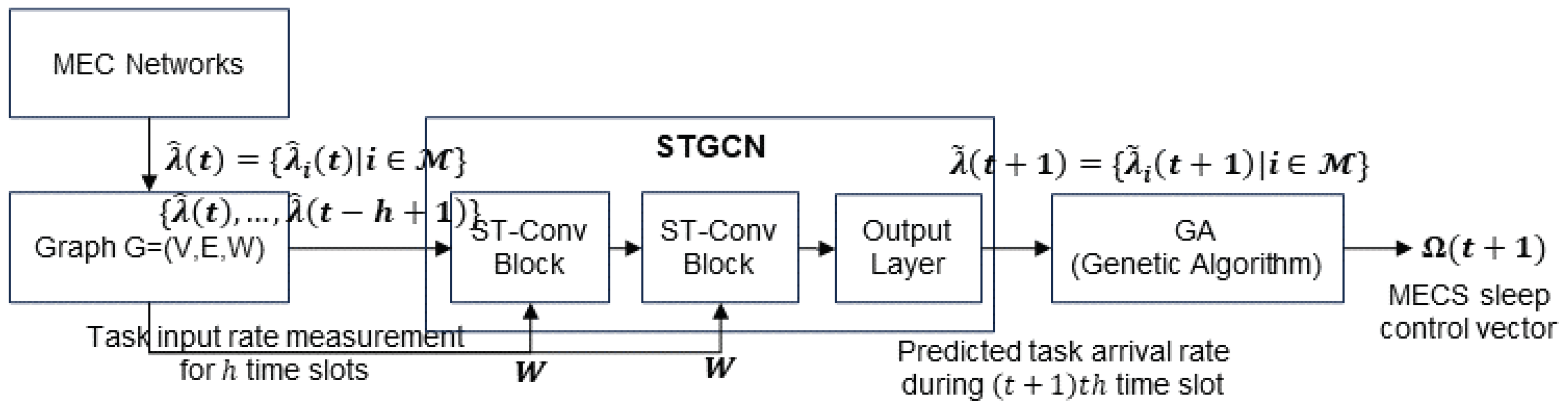
In Figure 1, we show the overall procedure of our MECS sleep control strategy. Our MECS sleep control method is composed of two modules. In the first module, at the beginning of each time slot t, a controller predicts $\{{\widehat{\lambda }}_i(t+1):i\in \mathcal{M}\}$ by using the spatio-temporal correlations among the recent past $\{\left\{{\widehat{\lambda }}_i\left(t\right)\right\},\left\{{\widehat{\lambda }}_i(t-1)\right\},\dots ,\left\{{\widehat{\lambda }}_i(t-h+1)\right\}\}$, where h is the length of the past task arrival rate history. We denote the predicted ${\widehat{\lambda }}_i\left(t\right)$ as ${\tilde{\lambda }}_i\left(t\right)$. The second module uses the genetic algorithm to determine the MECS sleep control vector $\Omega \left(t\right)$ by using ${\tilde{\lambda }}_i\left(t\right)$, $Q_i(t+1)$, and $F_i$, for all $i\in \mathcal{M}$. We explain the operation of each module in the following subsections.

Figure 1. Deep learning-inspired MECS sleep control framework.

4.1. Task Arrival Rate Prediction

The amount of tasks offloaded to an MECS i is determined by the number of users in $U_i\left(t\right)$ and their service preferences. Since the distance that a user can move during a time slot is limited, $U_i(t+1)$ is influenced mainly by $U_i\left(t\right)$ and $U_j\left(t\right)$s, where $j\in {\mathcal{M}}_i$. Therefore, ${\widehat{\lambda }}_i(t+1)$ is affected not only by $\{{\widehat{\lambda }}_i\left(t\right),\dots ,{\widehat{\lambda }}_i(t-h+1)\}$ but also ${\widehat{\lambda }}_j\left(t\right)$. Consequently, to increase the prediction accuracy, the spatio-temporal correlation among $\{{\widehat{\lambda }}_i\left(t\right),\dots ,{\widehat{\lambda }}_i(t-h+1)\}$ and ${\widehat{\lambda }}_j\left(t\right)$ must be exploited. To make use of the spatio-temporal relationship, we model an MEC system as a graph $G=(V,E)$. The set of nodes V is the set of MECSs $\mathcal{M}$. The elements of the edge set E are the links which reflect the adjacency between MECSs. In other words, the element $(i,j)$ in E is 1 if $j\in M_i$, otherwise it is zero.

Our goal is to predict the amount of tasks imposed on each MECS during the next time slot. Thus, we use the history of the workload generated in each $S_i$ as a node feature. We denote the node feature vector as $x\left(t\right)=\{{\widehat{\lambda }}_i\left(t\right):i\in \mathcal{M}\}$. Therefore, our task arrival prediction problem becomes a problem to find a mapping function $f_p$ such that

$$[{\tilde{\lambda }}_1(t+1),\dots ,{\tilde{\lambda }}_{\left|\mathcal{M}\right|}(t+1)]=f_p(G;[x\left(t\right),\dots ,x(t-h+1)]),$$

(6)

where h is the length of the task-load history.

Since an MEC system has a graph structure, we adopt a STGCN model to approximate $f_p$ by capturing and exploiting the spatio-temporal dependency among ${\widehat{\lambda }}_i(t-a)$s for all $i\in \mathcal{M}$ and $a\in \{1,\dots ,h-1\}$.

As we can see in Figure 1, STGCN is composed of two consecutive ST-Conv blocks and one output layer. The ST-Conv block is composed of a spatial Graph-Conv module in between two temporal Gated-Conv modules (Figure 2). The Gated-Conv module is composed of a 1-D convolution unit having a width $K_t$ kernel followed by GLU (gated linear unit). We denote the input to the k-th temporal Gated-Conv module in the l-th ST-Conv block as $v_{k,l}=(v_{k,l}\left(t\right),\dots ,v_{k,l}(t-h+1)$ where $k,l\in \{1,2\}$. Then, for each node in G, the 1-D convolution unit performs temporal convolution on $v_{k,l}$ by exploring $K_t$ neighbors, which reduces the sequence length from h to $h-K_t+1$. Two linear layers in the GLU take the temporal features extracted by the 1-D convolution unit and produces $P_{k,l}$ and $Q_{k,l}$, respectively. Then, GLU outputs $c_{k,l}$ by computing $P_{k,l}\odot \sigma \left(Q_{k,l}\right)$, where ⊙ is the element-wise Hadamard product. Therefore, if we denote the temporal convolution kernel for the k-th temporal Gated-Conv module in the l-th ST-Conv block as ${\Gamma }_{k,l}$ and the temporal gated convolution operator as ${\ast }_T$, the temporal gated convolution is expressed as

$$c_{k,l}={\Gamma }_{k,l}{\ast }_T{v}_{k,l}=P_{k,l}\odot \sigma \left(Q_{k,l}\right),$$

(7)

where $\sigma (·)$ is a sigmoid function.

Figure 2. ST-Conv block pipeline.

The spatial Graph-Conv module is designed based on a ChebNet [38], which is a spectral-based GNN. The goal of the spatial Graph-Conv module is to derive the spatial features from the temporal features extracted by the temporal Gated-Conv module. To achieve the goal, the spatial Graph-Conv module performs graph convolution on $c_{k,l}$. We denote the graph convolution operator as ${\ast }_g$ and the graph convolution kernel used by the spatial Graph-Conv module in the l-th ST-Conv block as ${\Theta }_l(l\in \{1,2\})$. We also denote the input size and the output size of the feature maps as $C_i$ and $C_o$, respectively. Since the output of the first temporal Gated-Conv module is fed into the spatial Graph-Conv module, the graph convolution on the input $c_{1,l}$ is given as

$${\Theta }_l{\ast }_g{c}_{1,l}=\sum _{i=1}^{C_i}{\Theta }_{i,j}\left(L\right)c_{1,l},1\le j\le C_o,$$

(8)

where ${\Theta }_{i,j}$ is the Chebychev coefficients and L is the normalized graph Laplacian.

Since the output of the spatial Graph-Conv module is fed into the second temporal Gated-Conv module, the final output of the l-th ST-Conv block becomes

$$v_{l+1}={\Gamma }_{2,l}{\ast }_T\mathrm{ReLU}\left({\Theta }_l{\ast }_g\left({\Gamma }_{1,l}{\ast }_T{v}_{1,l}\right)\right),$$

(9)

where ReLU is the rectified linear units’ function. The output of the second ST-Conv module is fed into the fully connected output layer. The output layer performs temporal convolution on the comprehensive features obtained from two ST-Conv blocks and produces a one-step prediction $\{{\tilde{\lambda }}_i(t+1):\forall i\in \mathcal{M}\}$.

To train the STGCN, the following L2 loss function is used.

$$L\left(\tilde{\lambda }\right|W_{\theta })=\sum _t\left|\right|\tilde{\lambda }(t+1)-\widehat{\lambda }(t+1){\left|\right|}^2,$$

(10)

where $W_{\theta }$ are all trainable parameters in the STGCN model.

4.2. MECS Sleep Control Vector Determination

After collecting $\{Q_i\left(t\right),{\tilde{\lambda }}_i\left(t\right),F_i:\forall i\in \mathcal{M}\}$ at the beginning of each time slot t, a controller determines an MECS sleep control vector by using GA. To exploit GA, we define a fitness function for a combination $x\in \Omega \left(t\right)$ as $f\left(x\right)=-E\left(t\right)$ if x satisfies the queue length constraint $Q_i\left(t\right)<Q_{th},\forall i\in \mathcal{M}$. When x violates the queue length constraint, we set $f\left(x\right)=-\infty$.

We create a population $X_c$ by randomly selecting n combinations from the possible combinations of $\Omega \left(t\right)$. Among the combinations in $X_c$, we find the best combination $x_c^{\ast }$ as follows.

$$x_c^{\ast }=argma{x}_{x\in X_c}f\left(x\right).$$

(11)

To construct a crossover set $Z_1$ from $X_c$, we create a temporary set Y by selecting the best $\lfloor n/2\rfloor$ combinations from $X_c$ based on the fitness values of $\forall x\in X_c$. Then, we randomly select two combinations x and y from Y and crossover them to make two children, $z_1$ and $z_2$. Specifically, we randomly select an index k from $[1,m]$, where $m=\left|\mathcal{M}\right|$ is the number of MECSs in an MEC system. Then, we make a child combination $z_1$ by concatenating $x[1:k]$ and $y[k+1:m]$, where $x[1:k]$ denotes the first k elements in x and $y[k+1:m]$ represents the last $m-k$ elements in y. We also make another child combination $z_2$ by concatenating $y[1:k]$ and $x[k+1:m]$ and put both $z_1$ and $z_2$ into the crossover set $Z_1$. To construct a mutation set $Z_2$, we mutate the children combination $z_1$ and $z_2$ as follows. After randomly selecting an index $k\in [1,m]$, we mutate $z_a(a\in \{1,2\})$ by changing $z_a\left[k\right]$ from 0 to 1 or vice versa. Then, we add the mutated $z_1$ and $z_2$ into the mutation set $Z_2$.

After repeating the crossover process and the mutation process $\lfloor n/2\rfloor$ times, we find the best combination $x_n^{\ast }$ in $X_c\cup Z_1\cup Z_2$. If $f\left(x_c^{\ast }\right)<f\left(x_n^{\ast }\right)$, we replace $x_c^{\ast }$ with $x_n^{\ast }$. We construct a new population $P_n$ by randomly choosing n combinations from $X_c\cup Z_1\cup Z_2$ and replace $P_c$ with $P_n$. We repeat the whole process $n_g$ times and output the final $x_c^{\ast }$ as ${\Omega }^{\ast }\left(t\right)$. We summarize the MECS sleep decision algorithm in Algorithm 1.

Algorithm 1 MECS Sleep Decision Algorithm
1:	At the end of a time slot t:
2:	Input: $\{Q_i\left(t\right),{\tilde{\lambda }}_i\left(t\right),F_i\}$, $\forall i\in \mathcal{M}$.
3:	Output: Optimal MECS sleep control vector $x_c^{\ast }$.
4:	Init: n, $n_g$.
5:	Construct $X_c$ by randomly selecting n elements from $\Omega \left(t\right)$.
6:	Get $x_c^{\ast }=argma{x}_{x\in X_c}f\left(x\right)$.
7:	$i=0$
8:	while  $i\le n_g$  do
9:	Create Y by choosing the $\lfloor n/2\rfloor$ elements in $X_c$ with the highest fittness value.
10:	$Z_1=Z_2=\varnothing$.
11:	$j=0$.
12:	for $j\le n$ do
13:	Randomly select x and y from Y.
14:	Make $z_1$ and $z_2$ by crossing over x and y.
15:	$Z_1=Z_1\cup \{z_1,z_2\}$
16:	Mutate $z_1$ and $z_2$.
17:	$Z_2=Z_2\cup \{\mathrm{mutated}{z}_1,\mathrm{mutated}{z}_2\}$
	Find $x_n^{\ast }=argma{x}_{x\in X_c\cup Z_1\cup Z_2}f\left(x\right)$
18:	if $f\left(x_c^{\ast }\right)<f\left(x_n^{\ast }\right)$ then
19:	$x_c^{\ast }=x_n^{\ast }$
20:	Construct $X_n$ by randomly selecting n elements from $X_c\cup Z_1\cup Z_2$.
21:	Replace $X_c$ with $X_n$
22:	Return $x_c^{\ast }$.

5. Performance Evaluation

In this section, we verify the proposed method via simulation studies. We compare the performance of our method with that of a conventional method using the LSTM model as a task arrival rate predictor.

5.1. Simulation Environment Setup

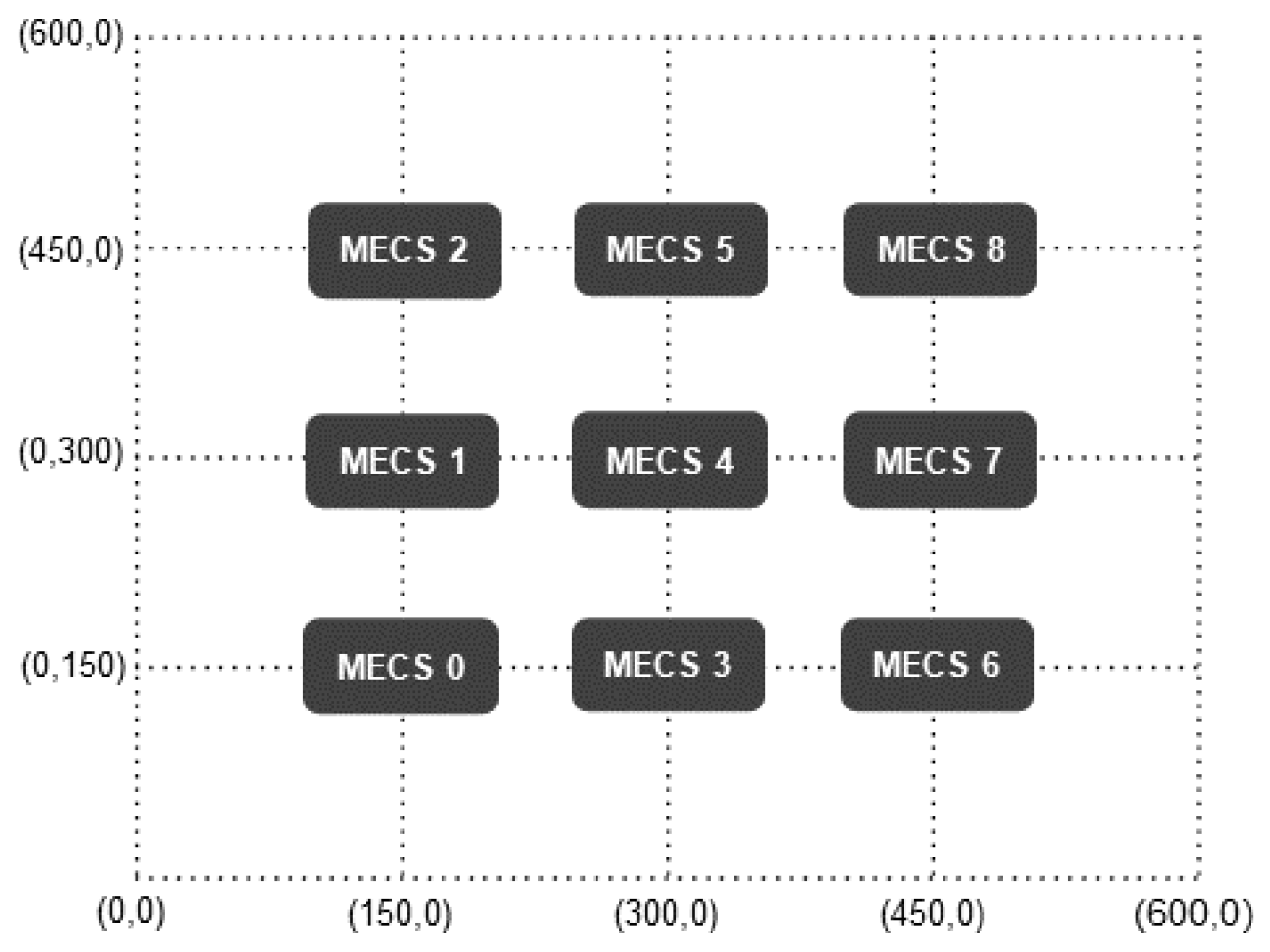
We deploy nine MECSs uniformly across a grid with dimensions of 600 m by 600 m (Figure 3). The service region of each MECS is configured as the surrounding four grids with itself at the center. At the beginning of the simulation, we uniformly deploy 275 users on the topology. Users move around over time according to a random mobility model. In other words, at the start of each time slot, a user changes its moving direction from $(0,2\pi ]$, according to the Uniform distribution, and selects its speed from the Normal distribution with a mean 15 m per time slot and a variance of $2.5$ m per time slot. To maintain the number of users in the topology, we assume that the top and bottom, as well as left and right, of the system topology are connected. Therefore, for example, when a user moves to the right and exits the topology, we add a new user to the left side of the topology.

Figure 3. Simulation topology.

Users offload their tasks to the nearest MECS. Initially, we configure that each user generates one task. After the initialization, we dynamically adjust the task generation rate of each user to change the total load imposed on the system over time. If $Q_i\left(t\right)\le Q_{th}$ for all MECS $i\in \mathcal{M}$ at the start of each time slot t, we increase the task generation rate of each user. The increase rate is randomly selected from $\{0.05,0.10,0.15,0.20\}$ for each user. When the load imposed on the MEC system exceeds its capacity, the queue length of at least one MECS exceeds $Q_{th}$. Then, after randomly choosing the decrease rate from $\{0.05,0.10,0.15,0.20\}$ for each user, we reduce the task generation rate of each user by the chosen rate. As the task arrival rate decreases, the number of sleeping MECS increases. However, in accordance with the second condition of the problem P1, at least three MECSs must remain active to serve users in the MEC system. Therefore, after the reduction in the task generation rate initiates, we consistently decrease the task arrival rate every time slot. This continues until the active MECS count reaches three. At this point, we resume increasing the user’s task generation rate by randomly selecting the increase rate from $\{0.05,0.10,0.15,0.20\}$ for each user every time slot.

After conducting the data generation process over 50,000 time slots, we construct the training dataset using task generation rates observed in the initial 35,000 time slots. The subsequent 7500 time slots are designated as the validation dataset, and the final 7500 time slots are allocated for the test dataset. In each dataset, a data sample is defined as a pair $\left(\right[x\left(t\right),\dots ,x(t-h+1)],x(t+1\left)\right)$, where $x\left(t\right)=\{{\widehat{\lambda }}_i\left(t\right):i\in \mathcal{M}\}$. These datasets are used to train the STGCN. After completing the training of STGCN, we generate $x\left(t\right)$ for 1000 time slots via the same data generation process. We then evaluate the performance of the proposed method by inputting them into the trained STGCN.

We set $P_m=20W$, $\alpha =0.5$, and $F_i=75$ tasks per time slot. We also set the maximum queue length of each MECS ($Q_M)$ to 75 and $Q_{th}=Q_M/2$. We configure the length of the task-load history as $h=12$. For the genetic algorithm, we set $n=\hspace{0.17em}|X_c|\hspace{0.17em}=20$ and $n_g=20$. We use the publicly known values of the LSM model and STGCN model for configuring their hyperparameters. Specifically, we use the hyperparameters in [39] to configure the hyperparameters of the LSTM model and employ the hyperparameters in [40] to configure the STGCN model. One hidden layer with 64 units is used for the LSTM model. Since one LSTM model has 16,961 parameters and there are nine MECS, a total of 152,649 parameters are used when the LSTM method is used. The STGCN model is composed of two ST-Conv blocks and one output layer. The units in the first ST-Conv block is (64, 32, 64) and the units in the second ST-Conv block is (64, 32, 128). The output layer has (256,128) units. Since one STGCN model is used for all MECSs, the total parameters when STGCN is used is 193,246. For our simulation study, we use the Colab Pro with CUDA version 12.0. We use Nvidia Tesla T4 GPU and 51 GB random access memory. When we run these models, we use Python version 3.10.12, Tensorflow 2.14.0, and Pytorch 2.1.0.

5.2. Task Arrival Rate Prediction Accuracy

To quantitatively compare the accuracy of the task arrival rate prediction, we calculate the mean absolute error (MAE) and the root mean square error (RMSE) and show the results in Table 3. We observe that STGCN can predict the task arrival rate more accurately than LSTM regardless of the location of an MECS in the topology. The difference stems from the fact that, unlike LSTM, which independently considers the temporal correlation of the task arrival rate at each MECS, STGCN comprehensively considers the spatio-temporal relationships of the task arrival rates across all MECSs when predicting the task arrival rate. For example, compared to the LSTM predictor, the STGCN predictor decreases MAE and RMSE by $11.24\%$ and $11.01\%$, respectively, when all MECSs are considered.

Table 3. Comparison of task arrival rate prediction accuracy. MECS 3 is located at the side, MECS 4 is located at the center, and MECS 8 is located at the vertex of the topology. Total represents the case where all the MECSs are considered when calculating MAE and RMSE.

	STGCN		LSTM
MECS	MAE	RMSE	MAE	RMSE
3	2.94	3.85	3.26	4.23
4	2.30	2.98	2.54	3.27
8	3.50	4.45	3.90	5.04
Total	3.00	3.88	3.38	4.36

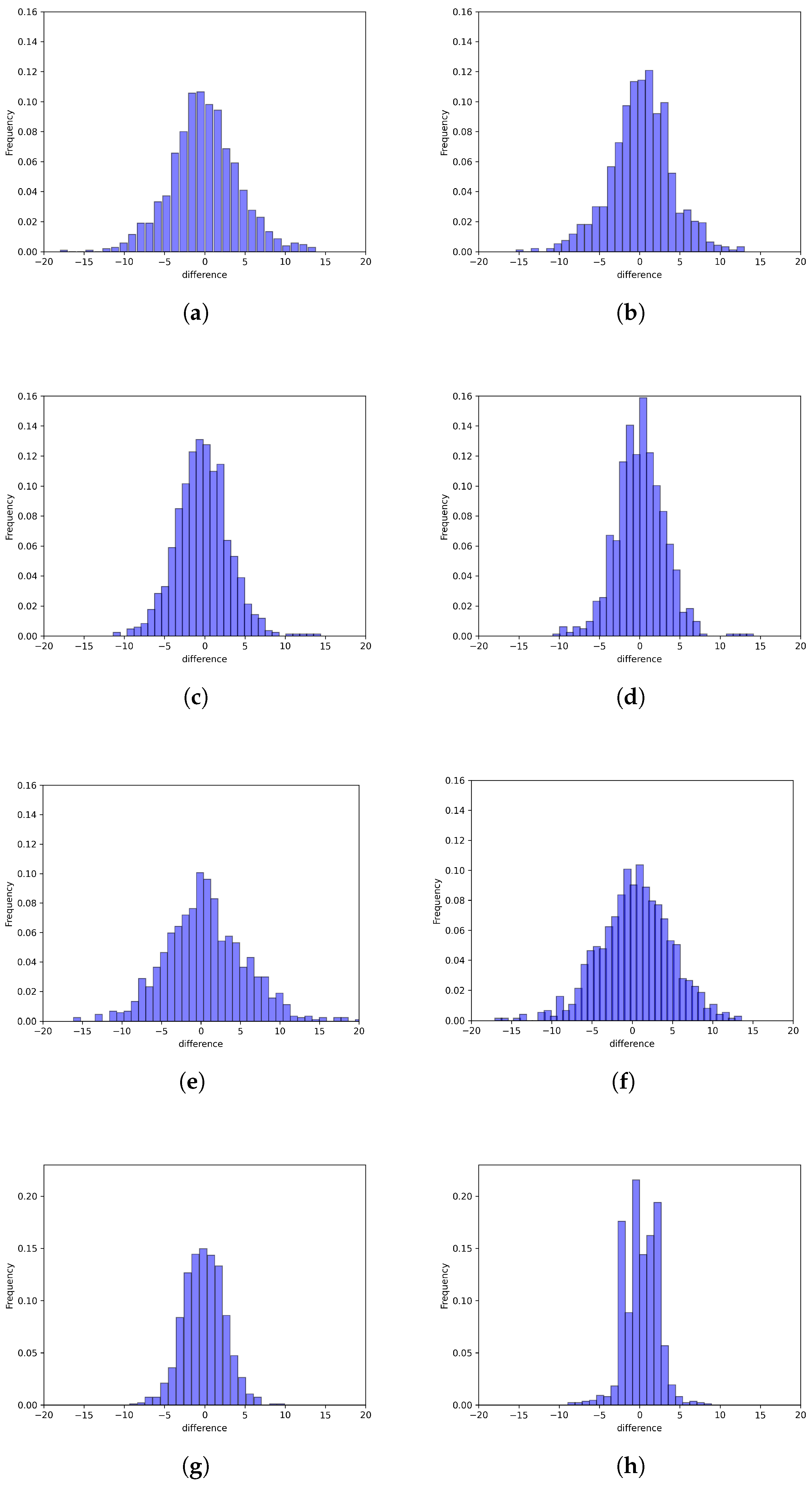
To further understand the prediction behavior, we inspect the distribution of the prediction error (i.e., ${\widehat{\lambda }}_i\left(t\right)-{\tilde{\lambda }}_i\left(t\right)$) in Figure 4. In this figure, for ease of visual comparison, we plot all subfigures with the same ranges for both the x-axis and y-axis. As we can see in Figure 4, the prediction errors are more densely clustered around zero when using STGCN compared to LSTM. In addition, we observe that STGCN exhibits smaller variations in the errors compared to LSTM.

Figure 4. Comparison of task arrival rate error distributions. The term ‘Total’ represent the case where all MECSs are considered. (a) LSTM, MECS 3, (b) STGCN, MECS 3, (c) LSTM, MECS 4, (d) STGCN, MECS 4, (e) LSTM MECS 8, (f) STGCN, MECS 8, (g) LSTM, Total, and (h) STGCN, Total.

We also examine the prediction delay. Since LSTM processes inputs sequentially, the LSTM method takes an average of 450 ms to predict task arrival rates. On the contrary, STGCN processes inputs in parallel by using graph convolutions. Therefore, the time required to predict task arrival rates decreases to as small as 10 ms when STGCN is used. This corresponds to a $93.33\%$ reduction compared to the LSTM method.

5.3. Performance of Sleep Control Vector Decision Method

We use GA to determine $\Omega \left(t\right)$. To focus on the influence of GA on the energy consumption and the queue length, we use true task arrival rates (i.e., $\left\{{\widehat{\lambda }}_i\left(t\right)\right\}$) instead of the predicted task arrival rates (i.e., $\left\{{\tilde{\lambda }}_i\left(t\right)\right\}$) when determining $\Omega \left(t\right)$ at the beginning of each time slot. Given ${\widehat{\lambda }}_i\left(t\right)$s, we compare the performance of GA and that of the exhaustive search (ES) method. Since ES explores all possible instances in the solution space, $\Omega \left(t\right)$ found by ES is globally optimal for the given input state.

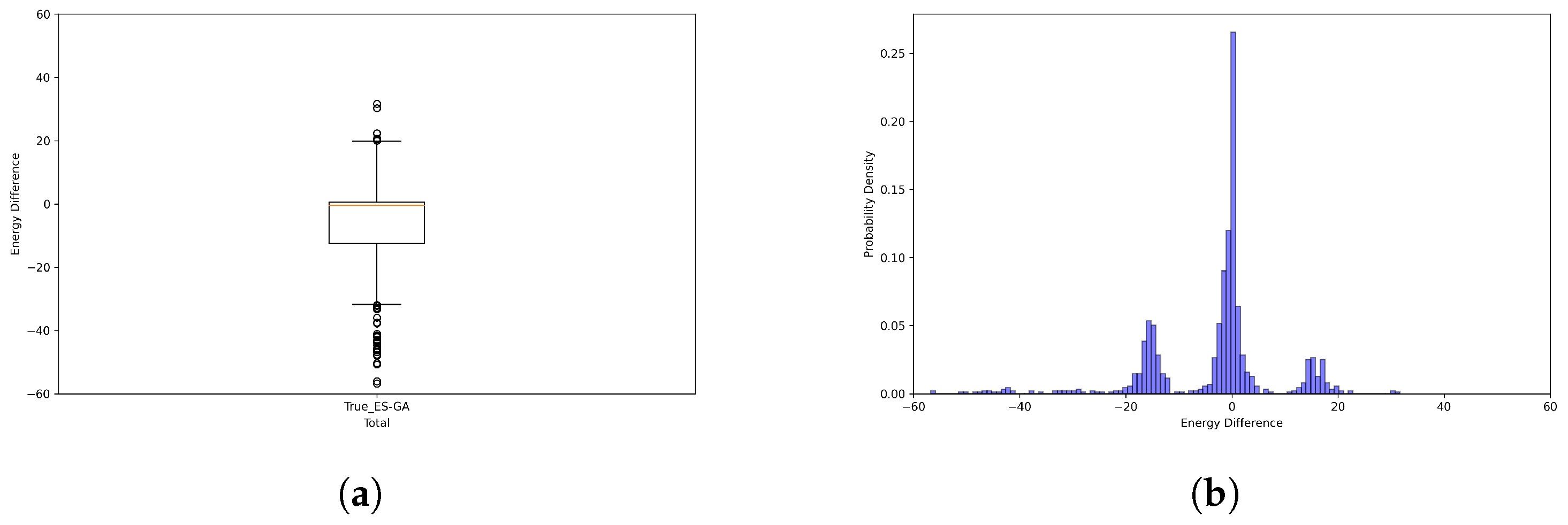
We measure the difference between $E\left(t\right)$ when ES is applied and that when GA is used and draw the distribution of the difference in $E\left(t\right)$ in Figure 5. The circles in the box plot (Figure 5a) represent the outliers. We observe that the distribution of $E\left(t\right)$ when GA is applied is very similar to that of $E\left(t\right)$ when ES is applied. Specifically, the Q-values in the box plot are $Q_1=-12.46$, $Q_2=-0.43$, and $Q_3=0.50$. In addition, we observe in Figure 5b that the difference in $E\left(t\right)$ is densely concentrated around zero. We also examine the Q-values of $E\left(t\right)$ when ES and GA were applied, respectively. When ES is used, it is $Q_1=8.53$, $Q_2=10.64$, and $Q_3=12.54$, but while GA is employed, it is $Q_1=8.61$, $Q_2=10.69$, and $Q_3=12.70$. Thus, the difference between Q-values obtained by GA and those when ES is applied is marginal.

Figure 5. Distribution of the difference in $E\left(t\right)$ between ES and GA. (a) Box plot; (b) Histogram.

In Figure 6, we show the distribution of the differences between the average queue length (i.e., $\overline{Q}\left(t\right)=\frac{1}{\left|\mathcal{M}\right|}{\sum }_{i\in \mathcal{M}}{Q}_i\left(t\right)$) when ES is applied and $\overline{Q}\left(t\right)$ when GA is utilized. When compared to the ideal case where the error is zero, the median value ($Q_2$) of $\overline{Q}\left(t\right)$ is 0.54. When we inspect the histogram, the average difference in $\overline{Q}\left(t\right)$ is 0.87. To further inspect the variance of $\overline{Q}\left(t\right)$, we examine the interquartile range (IQR), which is the difference between the 75th percentile and the 25th percentile. In the case of ES, the IQR for $\overline{Q}\left(t\right)$ is 4.40, whereas with GA, the IQR is 3.91, resulting in a difference of 0.49 between them. Considering that $Q_{th}=37.5$, such a difference can be regarded as very small.

Figure 6. Distribution of the difference in $\overline{Q}\left(t\right)$ between ES and GA. (a) Box plot; (b) Histogram.

We also compare ES and GA in terms of their run time. ES takes an average of 80 ms to find $\Omega \left(t\right)$ while GA takes an average of 29 ms. By using GA, we reduce the time needed to determine $\Omega \left(t\right)$ by $63.75\%$.

5.4. Combined Effect

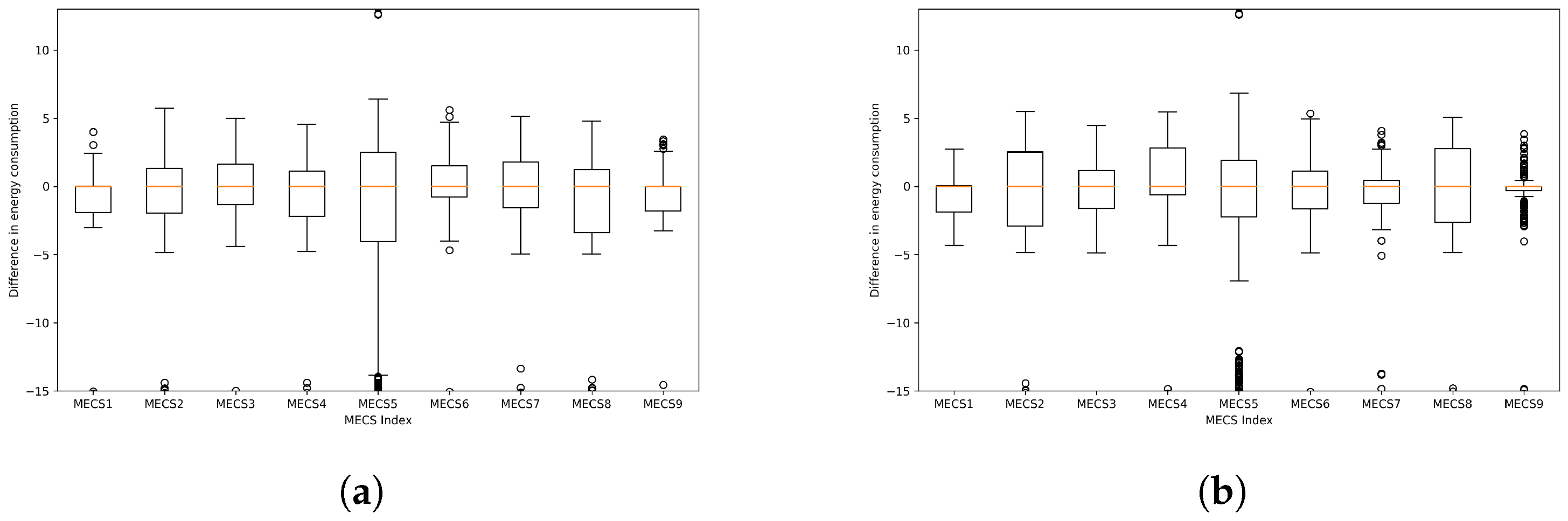
To evaluate the combined effects of the task arrival rate prediction and the sleep control vector determination, we compare the performance of the proposed method (STGCN-GA) with that of the following two techniques. The first method denoted by True-ES is an ideal method that determines $\Omega \left(t\right)$ via the exhaustive search by using the true task arrival rates $\left\{{\widehat{\lambda }}_i\left(t\right)\right\}$. The second method uses GA to determine $\Omega \left(t\right)$ by exploiting the task arrival rate predicted by the LSTM model. Henceforth, we denote the second method as LSTM-GA.

We denote the energy consumed at an MECS i during a time slot t when True-ES is used as $e_i^{TE}\left(t\right)$. We also denote by $e_i^{LG}\left(t\right)$ the energy consumed at an MECS i during a time slot t when LSTM-GA is used. We represent the energy consumed at an MECS i by our method during a time slot t as $e_i^{SG}\left(t\right)$. In Figure 7, we show the box plots of ${\delta }_i^{e,LG}\left(t\right)=e_i^{TE}\left(t\right)-e_i^{LG}\left(t\right)$ and ${\delta }_i^{e,SG}\left(t\right)=e_i^{TE}\left(t\right)-e_i^{SG}\left(t\right)$. To facilitate the comparison, the ranges of the y-axis in all subfigures are shown to be the same. We observe that the energy consumed by the proposed method is closer to the ideal value obtained by the True-ES method than the energy consumed by LSTM-GA. Specifically, $Q_2$ of ${\delta }_i^{e,LG}(\forall i\in \mathcal{M})$ is −0.52 while $Q_2$ of ${\delta }_i^{e,SG}(\forall i\in \mathcal{M})$ becomes −0.28. In addition, the IQR of ${\delta }_i^{e,LG}(\forall i\in \mathcal{M})$ is 14.10 and the IQR of ${\delta }_i^{e,SG}(\forall i\in \mathcal{M})$ decreases to 12.74.

Figure 7. Comparison of energy difference distributions for each MECS. (a) Box plots for ${\delta }_i^{e,LG}\left(t\right)$; (b) Box plots for ${\delta }_i^{e,SG}\left(t\right)$.

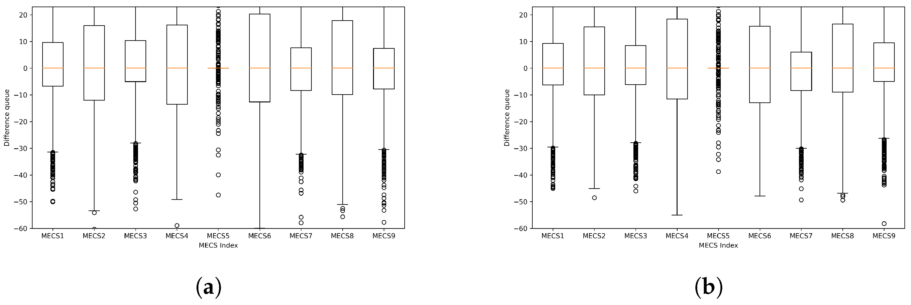
To investigate the difference between the queue length generated by our method and LSTM-GA and the ideal queue length generated by True-ES, we introduce the following symbols. We denote the difference between $\overline{Q}\left(t\right)$ obtained by True-ES and that acquired by our method as ${\delta }_i^{q,SG}\left(t\right)$. We also denote the difference between $\overline{Q}\left(t\right)$ obtained by True-ES and $\overline{Q}\left(t\right)$ when LSTM-GA is used as ${\delta }_i^{q,LG}\left(t\right)$. Then, we show the distribution of ${\delta }_i^{q,SG}\left(t\right)$ and ${\delta }_i^{q,LG}\left(t\right)$ in Figure 8. We observe that ${\delta }_i^{q,SG}\left(t\right)$ is closer to zero than ${\delta }_i^{q,LG}\left(t\right)$, which means that the proposed method makes the queue length more similar to the ideal $\overline{Q}\left(t\right)$ obtained by Tru-ES compared to LSTM-GA. Specifically, the median of ${\delta }_i^{q,LG}\left(t\right)$ is 0.56 while the median of ${\delta }_i^{q,SG}\left(t\right)$ is 0.47, which corresponds to a $16.07\%$ reduction. In addition, the IQR of ${\delta }_i^{q,LG}\left(t\right)$ is 4.20 while the IQR of ${\delta }_i^{q,SG}\left(t\right)$ is 3.87. Thus, the proposed method decreases the IQR of the queue length difference by $7.86\%$.

Figure 8. Comparison of queue length difference distributions. (a) Box plots for ${\delta }_i^{q,LG}\left(t\right)$; (b) Box plots for ${\delta }_i^{q,SG}\left(t\right)$.

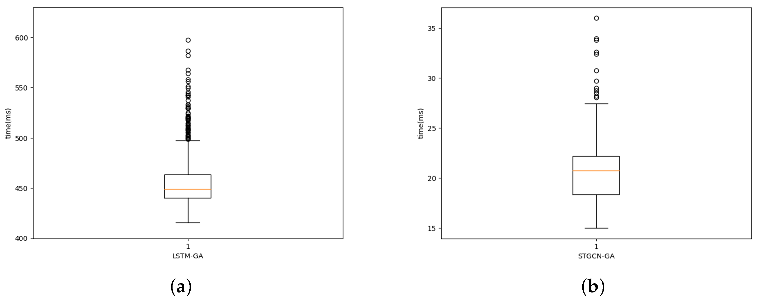
To compare the time taken for sleep control, we examine the end-to-end inference time, starting from predicting the task input rates to determining the sleep control vector. In Figure 9, we show the distribution of the end-to-end inference time as the box plots. When we inspect the Q-values, LSTM-GA obtains $Q_1=440$ ms, $Q_2=449$ ms, and $Q_3=463$ ms. The proposed method reduces the Q-values significantly. When our method is used, $Q_1=18$ ms, $Q_2=21$ ms, and $Q_3=22$ ms. In other words, compared to LSTM-GA, the proposed method decreases the median end-to-end inference time from 449 ms to 21 ms, which is a $95.32\%$ reduction. With respect to the IQR, our method reduces the IQR of the end-to-end inference time from 23 ms to 4 ms, which corresponds to an $82.16\%$ decrease.

Figure 9. End-to-end inference time distribution comparison. (a) LSTM-GA; (b) Proposed method.

6. Conclusions and Future Works

In this paper, we address the MECS sleep control problem in a multi-access edge computing system. To increase the energy efficiency of an MEC system while bounding the queue length of each MECS within a given value, we comprehensively exploit the spatio-temporal correlation structure in the task arrival rate distribution among the MECSs by using the STGCN model. By using only one STGCN model, we predict the task arrival rate for each MECS at the same time. In addition, we reduce the time to find an optimal sleep control vector given a system load state. We evaluate the performance of the proposed method via extensive simulation studies. The results verify that compared to a conventional method based on the LSTM model, the proposed method increases the energy efficiency of a system and decreases the average queue length.

As our future works, we will investigate methods to deal with the prediction error involved in the task arrival rate prediction. Any predictor introduces error inevitably. We will scrutinize the trend of errors that the STGCN predictor causes and analyze the tradeoff between energy consumption and queue length according to the type of errors. Then, we will study ways to improve the performance by controlling errors adaptively according to the operation state of an MEC system.