Population Dynamics in Genetic Programming for Dynamic Symbolic Regression

Abstract

This paper investigates the application of genetic programming (GP) for dynamic symbolic regression (SR), addressing the challenge of adapting machine learning models to evolving data in practical applications. Benchmark instances with changing underlying functions over time are defined to assess the performance of a genetic algorithm (GA) as a traditional evolutionary algorithm and an age-layered population structure (ALPS) as an open-ended evolutionary algorithm for dynamic symbolic regression. This study analyzes population dynamics by examining variable frequencies and impact changes over time in response to dynamic shifts in the training data. The results demonstrate the effectiveness of both the GA and ALPS in handling changing data, showcasing their ability to recover and evolve improved solutions after an initial drop in population quality following data changes. Population dynamics reveal that variable impacts respond rapidly to data changes, while variable frequencies shift gradually across generations, aligning with the indirect measure of fitness represented by variable impacts. Notably, the GA shows a strong dependence on mutation to avoid variables becoming permanently extinct, contrasting with the ALPS’s unexpected insensitivity to mutation rates owing to its reseeding mechanism for effective variable reintroduction.

1. Introduction

The integration of machine learning and artificial intelligence into various production systems, where data are continuously accumulated throughout the course of production processes, has become very common. This has led to the implementation of prediction models for various purposes, including estimating product qualities for accelerated product development, estimating the remaining useful lifetime of machines to facilitate timely maintenance scheduling, and acquiring comprehensive insights into production processes.

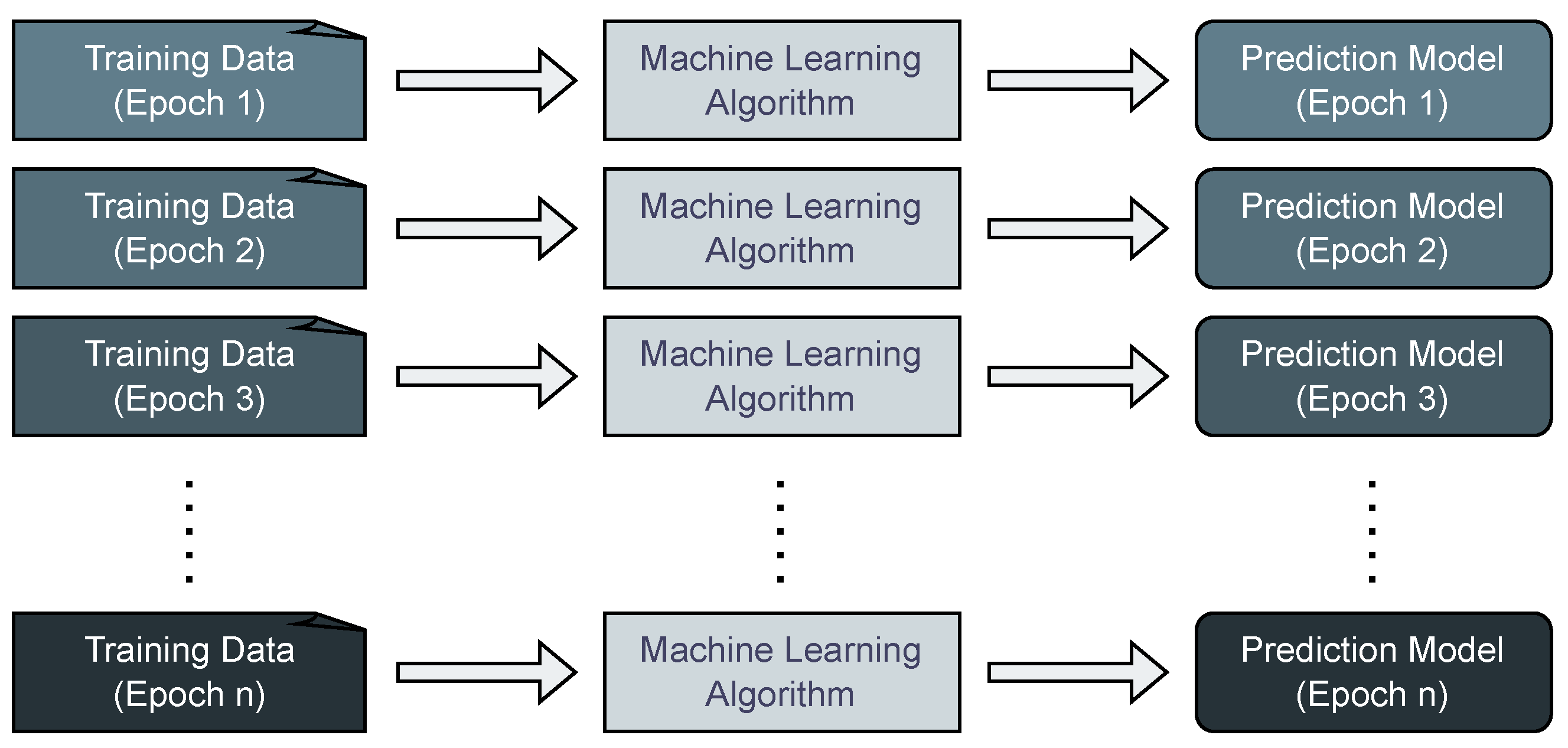
In the conventional paradigm of static machine learning scenarios, the process involves obtaining training data, training a prediction model using a machine learning algorithm, and subsequently utilizing the trained model, as illustrated in Figure 1. This approach involves aggregating data over an extensive time frame and applying it to machine learning algorithms to generate fixed prediction models. However, in scenarios where prediction models need to be adapted during the ongoing production process to account for shifts and regime changes, it becomes imperative to re-fit these models to the most recent data.

This necessitates a shift from static modeling to dynamic modeling, where the data are inherently dynamic, changing over time. Despite this dynamic nature, the modeling process remains essentially static, repeating over changing data, as illustrated in Figure 2. While faster classical machine learning algorithms like Random Forests [1] or Support Vector Machines [2] can be employed in such scenarios by simply re-executing them, slower algorithms like genetic programming (GP) [3,4] or training deep neural networks (NNs) [5] are often deemed impractical due to the runtime implications associated with their re-execution.

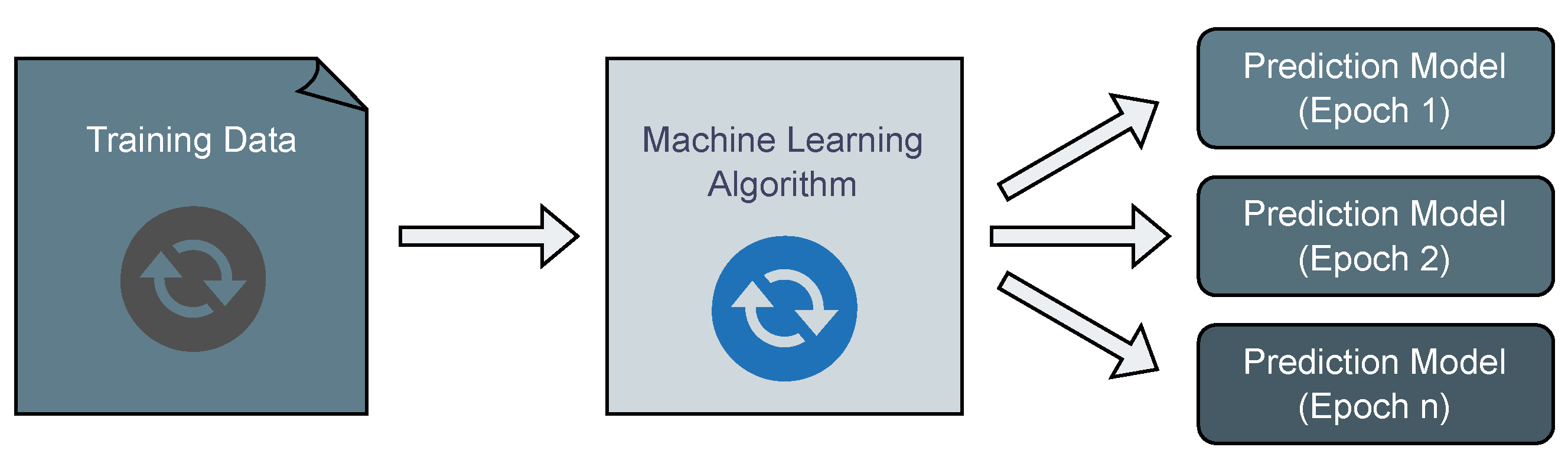
Rather than resorting to the complete re-execution of machine learning algorithms, a more efficient approach involves incorporating previous results to leverage existing knowledge, thereby reducing the runtime significantly. For instance, when using neural networks, one can optimize the network by seeding the re-optimization process with the weights of the latest model, rather than seeding it with new, random weights. In the realm of population-based evolutionary algorithms, these can operate in an open-ended fashion, continually evolving and adapting to changing datasets. In this dynamic modeling scenario, the training data are perceived as dynamic, changing over time, with the machine learning algorithm continuously running and outputting prediction models dynamically, as illustrated in Figure 3.

In industrial applications, the deployment of certain models is constrained due to their black-box nature. Notably, deep neural networks are often undesired as their predictions lack transparency, making it challenging for experts to comprehend the underlying prediction processes. This complicates the validation and interoperability of such models. On the contrary, white-box models, represented as symbolic models, are easily interpretable by humans, enabling validation by experts and enhancing the overall acceptance of machine learning models. The advantage of symbolic models lies in their simplicity, as they can be easily implemented in any system or programming language, given their nature as mathematical expressions. Additionally, symbolic models allow for various mathematical transformations such as simplifications and the definition of derivatives, providing additional benefits in specific scenarios.

In industrial use cases and production systems, the application of several models is sometimes limited due to their black-box nature. The aforementioned deep NNs are often undesired because experts do not want to rely on predictions where they do not understand the underlying prediction processes, and thus the validation and interoperability of a prediction model is difficult. On the other hand, white-box models, in the form of symbolic models, are easily readable by a human and can therefore be validated by an expert, which greatly improves the acceptance of a machine learning model. Having a symbolic model also allows for easy implementation in any system or programming language because it is, in essence, only a mathematical expression. Also, symbolic models allow for many mathematical transformations such as simplifications, or even the definition of a derivative, which can also be very useful in certain scenarios.

Symbolic regression (SR) via genetic programming (GP) emerged as a widespread approach for generating symbolic models. The underlying algorithm, a genetic algorithm (GA), evolves a population of symbolic models represented as expression trees [4]. While various forms of SR exist, this paper predominantly focuses on GP due to the suitability of population-based evolutionary algorithms in handling dynamic changes in datasets, aligning with their inspiration drawn from natural evolution and the adaptation of individuals to changing environments [6].

This paper centers its attention on two critical aspects: first, the consideration of a dynamic environment where training data evolve over time, and second, the exploration of symbolic models through GP as a promising means to address the evolving underlying optimization problem. In this context, the following research questions are addressed in this paper:

• How can changing training data be modeled within the context of a dynamic optimization problem?
• Can a dynamic symbolic regression problem be effectively solved using genetic programming?
• Which variants of genetic programming prove effective for dynamic symbolic regression problems?
• How do the population dynamics of GP evolve in the context of dynamic symbolic regression problems?

The term “dynamic” in the context of GP holds various meanings in different scientific papers. Noteworthy examples include the work of Macedo et al. [7] on the dynamic Santa Fe Ant Trail problem and that of Yin et al. [8], who applied GP in a dynamic real-world pricing environment. In these scenarios, the environment in which a GP solution operates is dynamic, but the solution itself remains unchanged. The aim is to find a single generalizing solution that performs well across various states of a dynamic system. This differs from the dynamicity explored in this paper, where different solutions emerge over time, tailored to short periods and becoming obsolete with system changes. Another aspect of dynamicity involves identifying dynamic systems as demonstrated by Quade et al. [9]. Here, GP is used to derive differential equations that best capture system measurements. Yet another dynamic facet includes GP’s self-adaptation, such as dynamically adjusting the population size during a run. However, these applications, while noteworthy, do not form the primary focus of this paper.

The exploration of GP for dynamic symbolic regression is still in its early stages, with limited attention. For instance, Macedo et al. [7] provides only a brief exploration of symbolic regression, while O’Neill et al. [10] concentrates on accelerating evolution in dynamic environments. This paper seeks to extend the scope of dynamic symbolic regression with GP, both in terms of the benchmark instances employed and the depth of analysis conducted, providing valuable insights into the inner workings of GP in dynamic contexts.

This paper is structured as follows. In the remainder of this section, we provide an introduction to the relevant concepts from the literature on genetic programming, symbolic regression, dynamic optimization problems, and open-ended evolutionary algorithms. Section 2 outlines the definition of dynamic symbolic regression used in this paper, offers a detailed description of the benchmark data, and explains the method for evaluating the results, including the experiment setup and variations for an in-depth analysis of GP aspects. Section 3 presents the results of the experiments, accompanied by detailed explanations, discussions on potential interpretations, and conclusions for each experiment. In Section 4, we discuss the findings and their implications and highlight the novel discoveries. Finally, Section 5 provides a brief summary of the findings and suggests future research activities.

1.1. Genetic Programming for Symbolic Regression

Symbolic regression (SR) is a subset of supervised machine learning, where regression models are expressed as symbolic mathematical representations [4]. Analogously, linear regression (LR) can be viewed as a subset of supervised machine learning, with a requirement that the model’s prediction remains linear in its parameters. While LR is efficiently solvable using least linear squares [11], achieving optimal models for symbolic regression proves to be a more intricate challenge.

The complexity stems from the dual challenge in symbolic regression (SR) where both the structure and numerical parameters of the symbolic model undergo optimization. Notably, optimizing the structure of symbolic models is recognized as an NP-hard problem, as the latest research suggests [12]. Additionally, optimizing the numerical parameters within a specific model structure is frequently framed as a real-vectored optimization problem. Although genetic programming (GP) is a prevalent choice for optimizing the model structure, enhancing the numerical parameters is often more effectively achieved through gradient-based numerical optimization methods [13].

The predominant approach for solving symbolic regression (SR) and acquiring symbolic models lies in the application of genetic programming (GP) [4]. GP, essentially an extension of genetic algorithms (GAs) [6], represents individuals as evolving expression trees over multiple generations. The fitness of an individual is assessed by an error metric, such as the mean squared error, calculated against a specific dataset. The genetic operators play instrumental roles in shaping the evolution of expression trees. The selection operator determines which individuals are chosen to become parents for the next generation based on their fitness. This ensures that genetic material from individuals with higher fitness contributes to the next generation, guiding the algorithm toward more favorable solutions. Crossover facilitates the interchange of subtrees between individuals. This process introduces diversity by combining genetic material from different individuals, potentially creating more adaptive and effective models. Moreover, the mutation operator introduces random changes to the numeric parameters, mathematical operators, or variables within an expression tree. This stochastic element allows for exploration of the solution space, preventing the algorithm from converging prematurely and promoting adaptability to the dynamic nature of the optimization problem.

Given the expansive nature of genetic programming beyond basic genetic algorithms, this paper does not delve into exhaustive reviews of GP, symbolic regression, or fundamental machine learning concepts. Interested readers are encouraged to explore other literature, such as the concise yet comprehensive Field Guide to Genetic Programming by Poli et al. [4]. For a more in-depth understanding, the initial work by Koza [3] and further exploration by Banzhaf et al. [14] provide additional insights into GP.

While alternative algorithms and variants for SR exist, such as stack-based GP [15], grammatical evolution [16], or non-evolutionary approaches [17], this paper deliberately focuses on GP.

As mentioned earlier, SR can be deconstructed into sub-problems for identifying a structure and optimizing numeric parameters. In our experiments, GP operates on both the structure and numeric parameters. However, numeric optimization is also employed to complement GP, as it often yields superior results compared to GP alone [18]. Generally, GP can be hybridized with various local optimization methods. For example, in scenarios where acquiring derivatives for gradient-based optimization is impractical or not feasible, derivative-free optimization methods like differential evolution could be employed.

To further guide GP and enhance efficiency, we impose constraints on the search space, including a maximum size for expression trees defined by the maximum number of nodes and the tree depth, along with restrictions on the allowed symbols through the defined grammar [19]. Detailed settings, including the population size, maximum generations, and other essential parameters, are outlined in subsequent sections detailing the experimental design.

While GP serves as the primary evolutionary algorithm for SR, other variants, such as the offspring-selection GA (OSGA) [20] and Age-Layered Population Structure (ALPS) [21], present alternative options. In this paper, we focus mainly on a basic GA and on the ALPS, because the ALPS seems to be especially suited to tackle dynamic optimization problems due to its reseeding mechanism. Multi-objective GA variants like NSGA-II [22] or SPEA2 [23] could also be considered, although they fall beyond the scope of this paper.

1.2. Dynamic Optimization Problems

Dynamic optimization can be understood as an extension to classic, static metaheuristic optimization that considers a time-dependent series of objective functions that have to be solved consecutively [24].

The general underlying assumption required for dynamic optimization is that solutions that performed well in previous iterations can either be adapted to the current objective or provide useful information to the optimizer. For GP on dynamic datasets, this assumption appears to be reasonable, as the introduction of singular new data points is unlikely to favor completely new expression trees with respect to most of the usual objective measures, like the RMSE, R${}^2$, or MAE.

Most academic benchmarks like the generalized Moving Peaks [25], the generalized dynamic benchmark generator [26], or the XOR-DOP generator [27] focus on vectors of decision variables [28] with occasional extensions toward robustness, constraints, large scales, or different types of changes with respect to predictability, impact, repetition, or whether or not the occurrence of the change is communicated to the optimizer. As an alternative, time-dependent versions of several popular combinatorial problems like the traveling salesman problem have been proposed [29,30].

To identify various states in a dynamic optimization problem, an identifier or counter is often used to denote the currently active version. This counter operates independently of inherent algorithmic counters such as iterations or generation counters, highlighting the autonomy of dynamic problem changes. To avoid potential naming conflicts with existing counters, we use the term epoch, signifying that usually numerous generations occur before an epoch change [31].

Epochs, representing the state of the dynamic optimization problem, and generations, indicating the algorithm’s progression, operate independently. In scenarios where dynamic optimization problems change slowly, the algorithm advances through multiple generations before an epoch change occurs. This is typical, as algorithms usually need time to converge. In contrast, in rapidly changing dynamic optimization problems, epochs may change faster than algorithm generations, resulting in multiple problem versions within a single generation. Consequently, evaluating an individual twice within a single generation could yield different fitness values if the epoch changes during the process.

The decision on when to implement an epoch change into the algorithm lies with the developer. To streamline the algorithm, epoch changes might be deferred to the beginning of the next generation, ensuring that all individuals within a generation are assessed under the same problem state. Alternatively, epoch changes could take effect immediately. For this paper, synchronization occurs at the start of a generation to avoid complications associated with fitness values stemming from multiple problem states, which could complicate the parent-selection process.

In practical scenarios, epoch changes are typically linked to real-world events, such as machine breakdowns or the introduction of new items. To synchronize the progression of dynamic optimization problems in benchmark instances, we utilize an epoch clock that interfaces with the algorithm to initiate an epoch change. Common epoch clocks include the following:

• Runtime clocks, where the epoch changes based on the algorithm’s elapsed duration;
• Generational clocks, which trigger an epoch change after a predetermined number of generations;
• Evaluation clocks, which initiate an epoch change after a predefined number of solution evaluations.

This paper employs generational clocks to avoid the challenge of altering the problem during the evaluation of individuals within a single generation.

1.3. Open-Ended Evolutionary Algorithms

Because continuous benchmark problems are quite prevalent in academic literature, a sizable portion of algorithms meant to tackle these are variations of particle swarm optimizations (PSOs) or differential evolution (DE) algorithms that are restricted or heavily geared toward those specific encodings [28,32].

A more flexible option that has been successfully employed is evolutionary algorithms that have been extended with features to address the dynamicity of the problem.

While evolutionary algorithms and especially GAs for static optimization are designed to converge toward a good solution, fully converged populations may have trouble adapting to new circumstances. Ideas to alleviate this issue range from change responses that generate new individuals [33], increase the mutation rates [34], or perform local searches to adapt current solutions. More refined approaches involve the self-adaptation of algorithm parameters in order to adapt to new situations [35].

Recently, research has indicated that simplistic, simple restarts of the optimizer or plainly specialized optimization algorithms might be sufficient to solve many dynamic optimization problems [36]. We therefore include a GA geared toward static optimization problems in our analysis.

Another feature of several dynamic optimization algorithms is the inclusion and explicit [37] memory structures like archives of solutions that are updated every few generations [38] or implicit [39] memory strategies that include structured and multi-populations or multiploid encodings with dominant or recessive genes [40].

The ALPS in this regard presents a fairly advanced combination of self-adaptive approaches and implicit memory via multiple populations, as it self-governs the number of populations it uses. These populations (layers) are additionally separated by age, and the solutions are periodically moved to higher (older) layers while the lowest (youngest) layer is re-initialized. This re-initialization involves reseeding the lowest layer with newly generated individuals, introducing a continuous stream of fresh genetic material. It serves as an additional mechanism, complementing mutation, to introduce diversity into the population. This structure avoids the issue of full convergence as new solutions are continuously generated and introduced, allowing the optimizer to store older solutions in higher layers and avoid having the new solutions directly compete with their seniors, giving them a chance to be refined before deciding whether the older solutions still outperform the new ones [21].

2. Materials and Methods

2.1. Dynamic Symbolic Regression

In standard regression problems, the relationship between independent variables $X_i$ and the dependent variable $y_i$ is established through a known or unknown generating function f that may involve certain parameters $\beta$:

$$y_i=f(X_i,\beta )+e_i,$$

(1)

where $e_i$ represents error terms like noise, and i denotes an observation. For static regression tasks, both the generating function f and the characteristics of independent features $X_i$ remain constant within reasonable margins.

However, in dynamic regression tasks, either the characteristics of the independent variables $X_i$ (such as their value range) or the generating function f can change over time. While alterations in the characteristics of independent variables may only impact the extrapolation behavior of a model, changes in the generating function f can disrupt any previously learned relationship between independent and dependent variables.

In this paper, we specifically explore dynamicity in regression tasks concerning changes in the generating function f while keeping the characteristics of independent variables fixed. We introduce a time-dependent hidden-state parameter $h_t$ to account for the time-dependent modification of the generating function. For instance, a dynamic regression instance might be characterized by the generating function:

$$f(X,h_t)=X_1·h_t+X_2,$$

(2)

where $h_t\in [0,1]$ controls the influence of variable $X_1$ while variable $X_2$ remains static.

The hidden-state variable $h_t$ serves as a control parameter for the speed of the shift, allowing for the simulation of abrupt concept changes if altered quickly or gradual concept drift if changed over an extended period. To facilitate the progression of the hidden-state variables for the evolutionary algorithm, we tie it to the epoch, which is increased after a predefined number of evaluations or generations are passed, as outlined in Section 1.2.

Adapting machine learning models to changes in the underlying data of a regression task is crucial, as changes may render previously significant variables less important or entirely irrelevant. Variables might also interact differently, affecting the model’s ability to predict the target. Also, the learned relationship between old inputs and targets may no longer hold. In the realm of evolutionary algorithms, particularly genetic programming (GP), this translates to a probable decline in the quality of individuals after data changes, resulting in an overall decrease in population quality.

The magnitude of this quality drop depends on the nature of the data change. Limited changes or additions to observations might lead to a relatively small drop in quality, while alterations in variable interactions can cause more pronounced drops. Following such drops, the algorithm’s task is to adapt, identifying new individuals that align better with the new data. Depending on the extent of the data change, GP can leverage genetic material from the previous generation rather than entirely rebuilding the population. This adaptive approach enables GP to efficiently navigate dynamic data scenarios.

2.2. Benchmark Data

To investigate the performance of various algorithms, we provide different benchmark instances. These synthetic benchmarks not only serve as a means of evaluation but also provide the base for a detailed analysis of the algorithmic behavior in dynamic scenarios.

In this paper, we use five different problem instances drawn from two sources. In all cases, the distributions for the independent variables remain fixed, and the generating function comprises various terms of these independent variables. Depending on the hidden-state variable, certain terms are consistently present, while others may be gradually or abruptly enabled and disabled over time.

The first three benchmark instances are adapted from the work of Winkler et al. [41] to suit a dynamic optimization environment. These instances are defined as follows:

$$\begin{array}{cc}\hfill W1(x,h)& =x_1\left(h{x}_2+\left(1-h\right)x_3\right),\hfill \end{array}$$

(3)

$$\begin{array}{cc}\hfill W2(x,h)& ={\alpha }_2\left(x_1{x}_2+x_3{x}_4\right)+{\beta }_2\left(h{x}_5{x}_6+\left(1-h\right)x_7{x}_8\right)\mathrm{and}\hfill \end{array}$$

(4)

$$\begin{array}{cc}\hfill W3(x,h)& ={\alpha }_3\left(x_1{x}_2{x}_3+x_4{x}_5{x}_6\right)+{\beta }_3\left(h{x}_7{x}_8+(h-1)x_9{x}_{10}\right),\hfill \end{array}$$

(5)

where $\alpha$ and $\beta$ scale the respective terms to have equal variance. All input variables $x_1\cdots x_{10}$ are drawn from a uniform distribution $\mathcal{U}$ between 1 and 10.

To enable gradual transitions between states, as outlined in the original paper, we employ a substantial number of epochs, progressively adjusting the hidden-state variable h in each epoch. The state changes unfold over multiple epochs, featuring abrupt, fast, and slow transitions from zero to one, and vice versa. This dynamic evolution is precisely defined by the following sequence:

$${\left[1\right]}_{100}{[1\to 0]}_{10}{\left[0\right]}_{100}{\left[1\right]}_{100}{[1\to 0]}_{50}{\left[0\right]}_{100}{[0\to 1]}_{20}{\left[1\right]}_{50}{\left[0\right]}_{100}{[0\to 1]}_{10}{\left[1\right]}_{10}$$

Here, ${\left[a\right]}_n$ denotes a constant value of a for a duration of n epochs, while ${[a\to b]}_n$ indicates linearly spaced values between a and b over the course of n epochs. The visual representation of this progress is depicted in Figure 4.

The next two benchmark instances draw inspiration from the benchmark generation procedure proposed by Friedman [42], adapted for dynamic optimization. Unlike the single hidden state employed in the previous benchmarks, the Friedman-based benchmarks involve three states $\left(h_{t,a},h_{t,b},h_{t,c}\right)=h_t\in {[0,1]}^3$, each independently controlling specific terms.

The data for each term i are generated independently using the random function generator described by Friedman [42], denoted as $X_i$ and $F_i^{*}\left(X_i\right)$, representing the calculated target by the generator. The final target is derived as the weighted sum of the term targets, with their state factors incorporated:

$$y=F(X,h)=\sum _{i=1}^{i\le 3}(F_i^{*}\left(X\right)h_i-{\mu }_i)/{\sigma }_i,$$

(6)

where i represents the terms, and the mean ${\mu }_i$ and standard deviation ${\sigma }_i$ of the generated targets for each term are utilized to normalize the generated targets before summation. The inputs per term are concatenated, and the variable names are assigned according to the term, with a letter and a number denoting the nth variable of the term (e.g., ${\mathrm{a}}_1,{\mathrm{a}}_2,\cdots ,{\mathrm{b}}_1,\cdots$), resulting in the total training inputs.

The Friedman benchmark-generating procedure enables the control of the number of input features per term and the amount of noise. A higher number of features increases the instance’s difficulty due to the increased size of each term. For this paper, we omitted the use of any noise, setting the noise parameter to $0.0$.

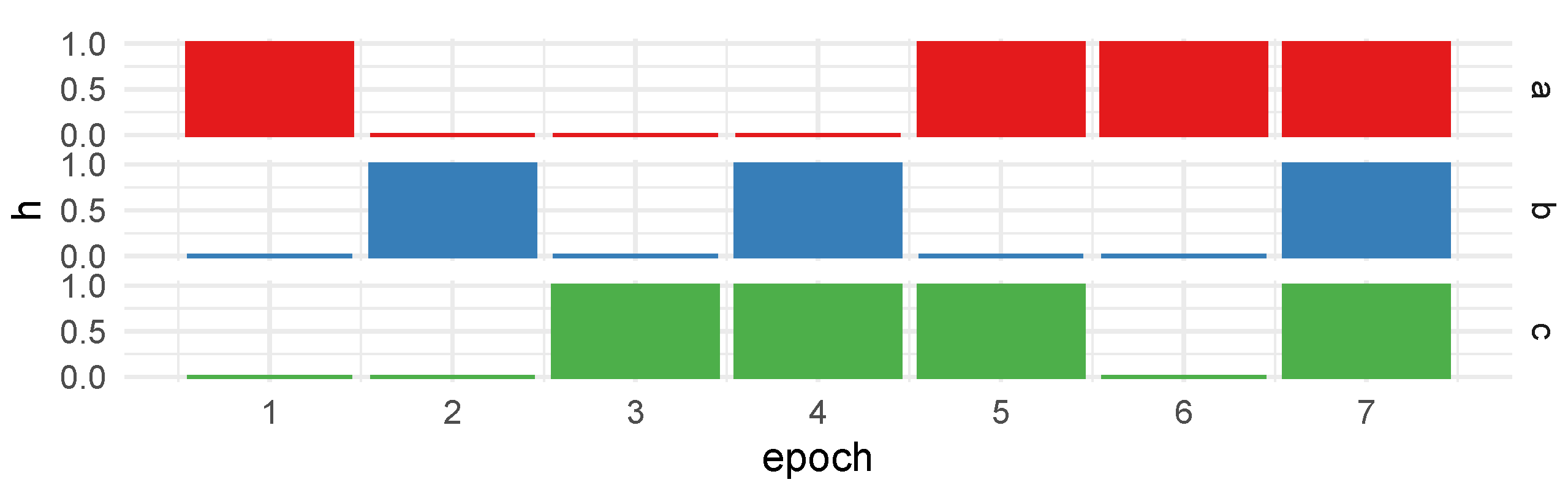
In the case of Friedman-based benchmarks, we only implement abrupt state changes with a limited number of epochs. This deliberate choice ensures a slower epoch clock, allowing ample time for evolution before each epoch change. The progression unfolds as follows:

$$\left[\begin{array}{c}1\\ 0\\ 0\end{array}\right]\left[\begin{array}{c}0\\ 1\\ 0\end{array}\right]\left[\begin{array}{c}0\\ 0\\ 1\end{array}\right]\left[\begin{array}{c}0\\ 1\\ 1\end{array}\right]\left[\begin{array}{c}1\\ 0\\ 1\end{array}\right]\left[\begin{array}{c}1\\ 0\\ 0\end{array}\right]\left[\begin{array}{c}1\\ 1\\ 1\end{array}\right]$$

This sequential progression ensures that the machine learning algorithm encounters individual terms first (epochs 1 to 3), explores combinations of two terms (epochs 4 and 5), briefly reverts to a single term (epoch 6), before finally activating all terms (epoch 7), as illustrated in Figure 5. The rationale behind this strategy is to provide the algorithm with opportunities to analyze individual terms initially and assess its ability to remember them when activated later. Additionally, the last epoch serves as a test of the algorithm’s capability to handle two new terms simultaneously, resulting in the presence of all three terms.

The combination of benchmark sources, comprising the Winkler-based benchmarks and Friedman-based benchmarks, includes a total of 5 instances, each presenting distinct levels of difficulty. The details of these instances, along with the training and test sizes, are summarized in

Table 1. Overview of the parameters of the used benchmark instances.

Name	Type	Train. Size	Test Size	Features	Complexity
W1	Winkler et al. [41]	100	10	3	low
W2	Winkler et al. [41]	100	10	8	low
W3	Winkler et al. [41]	100	10	10	medium
F1	Friedman [42]	1000	100	3	high
F2	Friedman [42]	1000	100	6	high

.

The complexity is a qualitative measure that provides a rough description of the generating functions’ complexity, considering the number of variables and the complexity of the employed mathematical operators and their interactions. It is worth noting that, while the number of training and test rows might appear relatively modest for the Winkler-based benchmarks, the design compensates with a relatively high number of epochs that facilitates the gradual shifts. This design choice is similar to a mini-batch training paradigm, where the same generating function is employed for each mini-batch.

2.3. Population Dynamics

Given that benchmark instances are generated based on a sum of weighted terms, our aim is to analyze the presence and significance of these terms within the current population. While an exact occurrence analysis using subtree matching would be challenging, especially for complex generating functions such as those in Friedman-based benchmarks, we approach our analysis based on the known variables for each term. Our focus lies on two aspects:

• Variable frequency, measuring the relative occurrence of a variable within the entire population.
• Variable impact, measuring the importance of a variable, based on Breiman [1]’s permutation feature importance.

The variable frequency is computed across the entire population, while variable impacts are defined on an individual basis. The impact of a variable is determined by measuring the reduction in a model’s accuracy when the variable is absent from the dataset. This absence is simulated by shuffling the variable, disrupting its relationship with the target and other correlated inputs. To obtain variable impacts for the entire population, we calculate the mean impact over all individuals for each feature. Importantly, we bear in mind the fact that individual feature importance essentially measures the drop in model accuracy, and low-accuracy models will contribute less to the overall impact. Thus, the impact calculated over the population is not inflated by models with low accuracy. Alternatively, scaling the impact with model accuracy is possible, but it could lead to a doubly scaled measure.

In summary, variable frequency indicates the presence of terms in the population, irrespective of their relevance to the regression task. On the other hand, variable impacts assess the importance of terms for the current regression task. In a well-behaved GP scenario, the population should converge toward solutions with high impacts, maintaining a steady frequency for variables of high impact while dropping out variables with no importance.

The interplay between the variable frequency and impacts allows us to analyze whether GP can initially identify useful variables and subsequently adapt to changing scenarios. Adaptation may involve the following:

• Increasing the frequency of variables gaining importance due to different scenarios;
• Decreasing the frequency of variables no longer relevant due to a change in the scenario.

Considering the correct usage of variables in terms of the model structure, we hypothesize that variable impacts tend to increase slowly over time during GP convergence but can drop instantly in the face of an abrupt shift in the dynamic problem. In contrast, variable frequencies should change slowly, either gradually increasing for relevant variables or decreasing for variables that are no longer relevant.

2.4. Experiment Setup

The dynamism in the dynamic regression problem is controlled through the progression of epochs, necessitating careful configuration of the epoch clock in alignment with the algorithm. This configuration is crucial for accommodating the different characteristics of different benchmark instances. For instance, in the case of Winkler-based benchmarks, which conceptually embody only a few states, we employ a substantial number of approximately 700 epochs to facilitate the transition between two states, allowing for gradual shifts. In contrast, the Friedman-based instances incorporate only 7 epochs, each spanning an extended duration. To illustrate, the Winkler-based benchmarks may adopt an epoch clock synchronized with each generation, allowing for a finely tuned paradigm shift. On the other hand, the Friedman-based instances might opt for an epoch clock setting of 100 generations or more for a single epoch change. The algorithm parameters for each benchmark instance are detailed in

Table 2. Experiment parameters for all algorithms and instances.

		W1	W2	W3	F1	F2
GA and ALPS	Epoch Clock (Generational Interval)	1	1	1	150	250
	Max Tree Length	25	50	70	70	100
	Creator	Probabilistic Tree Creation
	Mutation	Change Node Type, Full Tree Shaker, One Point Shaker, Remove Branch, Replace Branch [4]
	Mutation Probability	15%
	Crossover	Subtree Swapping [4]
	Crossover Probability	100%
	Function Set	$+,-,*,/,\mathit{var},\mathit{const}$
	Local Numeric Opt.	Levenberg–Marquardt, 10 iterations [43]
GA	Population Size	100	200	500	200	500
	Elites *	1	1	1	1	1
	Selector	Prop.	Tour. (k = 3)	Tour. (k = 4)	Tour. (k = 3)	Tour. (k = 4)
	Maximum Generations	700	700	700	1500	2000
ALPS	Max Layers	10	10	10	10	10
	Population Size (per Layer)	100	100	100	100	100
	Elites * (per Layer)	1	1	1	1	1
	Selector	Generalized Rank (Pressure = 4)
	Age Gap	20	20	20	20	20
	Aging Scheme	Poly	Poly	Poly	Poly	Poly
	Maximum Generations	700	700	700	1500	2000

* Elites are reevaluated every generation because their quality may change as a result of an epoch change.

. While specific experiments presented later involve variations in certain parameters, the foundational configurations are outlined in the base experiment parameters.

We intentionally opted for a generational clock rather than an evaluation clock, even though the overall population size for the ALPS changes during the run, leading to an increase in the number of evaluations per generation over the algorithm’s duration. This choice was made to facilitate a more straightforward comparison. In most cases, the ALPS begins with a smaller overall population than the GA but increases as new layers open. Consequently, the total difference in the number of evaluations for the GA and ALPS varies to some extent for each epoch but tends to average out over the entire algorithm run. For instance, consider the F2 instance, which is solved by a GA with a population of 500 for 2000 generations, resulting in approximately 1,000,000 evaluations. In contrast, the ALPS starts with 100 individuals and allows for a maximum of 10 layers that open dynamically, totaling around 1,600,000 evaluations. While the authors acknowledge this difference, we believe that our conclusions remain valid without extensively parameterizing the algorithms to precisely match the number of evaluations.

2.5. Experiment Variation

In the subsequent sections, we introduce variations of the previously described experimental setup to analyze specific facets of GP for dynamic SR. These experiment variations will also be referenced later in distinct result sections corresponding to their respective experiment variants. Although these experiments were conducted and analyzed independently of the base experiments, their motivations frequently trace back to research questions that emerged during the analysis of other experiments.

2.5.1. Faster Epoch Changes

The findings from the base experiment that will be discussed in Section 3.1 indicate that GP generally performs well in handling changes in epochs when given sufficient time to adapt. This variant experiment seeks to investigate whether faster epoch changes pose a greater challenge for GP. In addition to the “Normal” speed, we introduce two new speeds, namely, “Fast2” and “Fast3”, for each benchmark instance, accompanied by adjusted configurations to accelerate the epoch changes, as listed in

Table 3. Experiment parameters for analyzing the impact of fast epoch changes. The table lists only the modifications from the base experiments, with the three values separated by “/” indicating the configurations for Normal speed and the Fast2 and Fast3 variants.

		W1	W2	W3	F1	F2
GA	Epoch Clock (Generational Interval)	1/1/1	1/1/1	1/1/1	150/75/50	250/100/67
	Population Size	100/50/33	200/100/67	500/250/167	200/200/200	500/500/500
	Maximum Generations	700/700/700	700/700/700	700/700/700	1500/750/500	2000/1000/670
ALPS	Epoch Clock (Generational Interval)	1/1/1	1/1/1	1/1/1	150/75/50	250/100/67
	Population Size (per Layer)	100/50/33	100/50/35	100/50/33	100/100/100	100/100/100
	Maximum Generations	700/700/700	700/700/700	700/700/700	1500/750/500	2000/1000/670

. On one hand, we reduced the frequency of the generational clock to hasten the epoch changes, and on the other hand, we adjusted the population size to indirectly accelerate the epoch changes.

2.5.2. Mutation Rate

Analyzing the variable frequencies in the overall results in Section 3.1 reveals that GP retains genetic material for all the relevant variables, even when they are not actively used at certain points in time. It appears that mutation plays a crucial role in maintaining diversity and reintroducing dormant variables when needed later in the evolutionary process. This experiment seeks to examine the extent to which mutation is necessary to enable GP to rediscover relevant variables or if mutation is indispensable for this purpose. The modified experiment and the adjusted mutation rates are given in

Table 4. Parameters for the experiment analyzing varied mutation rates. The table contains only modifications made to the base experiments.

	W1	W2	W3	F1	F2
Mutation Probability	15%/10%/5%/1%/0.5%/0.1%/0.05%/0.01%/0.005%/0.001%/0.0%

.

3. Results

The following results are grouped based on the distinct experimental configurations, each aimed at analyzing various facets of GP for dynamic SR. We begin with the genera outcomes derived from the base experimental setup detailed in Section 2.4.

3.1. Base Experiment Results

We initially assess the algorithms’ effectiveness over the runs. In contrast to static optimization problems, a singular conclusive metric for the best solution is not provided, given the dynamic nature of the problem, where older metrics become obsolete with changes to the problem. The most relevant metric is the quality of the current best individual within the population at a specific generation, offering insight into the algorithm’s optimal performance given the current state of the dynamic optimization problem. Additionally, we present the current mean quality of the population, providing an overview of the algorithm’s general state and its convergence status.

Figure 6 illustrates the mean population quality and best quality (measured in Pearson R${}^2$) over time for each algorithm across different problem instances. It is evident that, for all instances, the best solution over time predominantly reaches 1.0 R${}^2$ exactly or very close, indicating that the algorithms consistently discover high-quality models. Notably, regular dips in the average quality coincide with epoch changes. This pattern is particularly noticeable in the Friedman-based instances (F1 and F2), where the data transition abruptly compared to the more gradual changes in the Winkler-based instances (W1, W2, and W3). For the Friedman-based instances, variations in the difficulty among the epochs are apparent, with a lower average quality indicating greater challenges in obtaining good models. In these cases, even the best solutions found do not consistently achieve a perfect 1.0 R${}^2$.

For the ALPS, recurring drops in the average quality align with the reseeding of layer zero. Due to this reseeding mechanism and the population growth over time, the ALPS exhibits a lower overall population quality compared to the GA. Although comparing only the top layer of the ALPS to the GA might yield similar results, we deliberately opted to analyze the total ALPS population to more accurately reflect the actual dynamics of the ALPS.

The results suggest that, for the presented problem instances, the algorithms quickly adapt to changes in the training data within a few generations. This rapid adaptation could imply that the difficulty for individual epochs was generally low. However, challenges persist in the last phase for both Friedman-based instances, where the algorithms struggle to fully solve the problem. It is worth considering that these challenges may also arise from imposed limitations on the tree size, potentially rendering the problem unsolvable within the given constraints.

Figure 7 depicts the average variable frequencies within the population across all runs for each algorithm and instance. This visualization offers insights into the variables retained in the population and how their relative frequencies change in response to epoch variations. The shifts in the population composition are clearly observable in all instances, aligning well with the epoch changes.

Similar to the quality dynamics, we can readily observe the reseeding pattern in the ALPS, which aims to normalize the overall frequencies by evenly distributing newly generated individuals in layer zero. However, the impact of reseeding typically normalizes after a few generations.

Beginning with the W1 instance, we observe that all the variables are initially equally distributed in the population, adjusting over time in response to the dynamic nature of the benchmark. While variable x1 maintains a relatively constant frequency, x2 and x3 undergo cycles corresponding to the changing relevance dictated by the benchmark’s underlying function and epoch shifts (as defined earlier in Figure 4). The variable frequency changes exhibit different speeds, reflecting the gradual or abrupt nature of the state changes over epochs. However, these changes occur steadily and slowly, spanning multiple generations rather than happening instantaneously.

The overall patterns for instances W2 and W3 closely resemble W1, albeit with slightly more fluctuations due to the increased number of variables. In cases where multiple variables of a single term are tuned down during epoch progression, their occurrences in the population decrease concurrently.

In the F1 instance, we observe a mix of relevant variables. For the initial three epochs, the variables operate independently, as defined in Figure 5. The subsequent epochs introduce combinations of two terms, and the last epoch displays an equal distribution of the variables when all the terms are relevant. A similar observation holds for the F2 instance but with two variables per term.

Similar to the variable frequencies over time, Figure 8 illustrates the impacts (as defined in Section 2.3), representing the usefulness of the variables in predicting the target. A notable observation is that the impacts do not all start at the same initial value, reflecting instances where the generating function does not use all the variables in the first epoch.

Another significant difference from variable frequency is the rapid change in impacts, reflecting how quickly solutions change their behavior with new problem data after an epoch change. For example, in benchmark W1, the drop in variable impact at generation 210 and around 540 is abrupt, while the shift from generation 310 to 350 occurs more gradually, leading to slower changes in the variable impacts.

In the Friedman benchmarks, where all the epoch changes are abrupt, this characteristic is even more evident. However, due to the nature of the underlying function generating the target value for the benchmark instances, it is observed that the impacts of the variables differ, even when all are relevant for the model. This discrepancy arises when different terms or subtrees contributing to the target value have varying value ranges, contributing to the final target to different degrees. Consequently, benchmarks with a higher number of features, especially F2 and F3, become challenging to interpret due to the variables having different maximum impacts.

Even in the separated figures for the variable frequency and impacts, there is a clear indication of a close relationship between the two. This aligns with the intuitive understanding of these measurements, where variable impacts assess the immediate usefulness of variables, while the variable frequency reflects the consequence of the model’s fitness, with the fitness closely related to identifying variables with a high impact.

To better analyze the relationship between these two measurements, we focus on a single problem instance where we can plot the variable frequency and variable impact of individual variables for closer inspection. Figure 9 illustrates the relation between the frequency and impact over time for the instance W1. It is evident for variables x2 and x3 that the variable frequency (red) typically follows the variable impacts (blue). While this result is not surprising, it reaffirms the intuitive notion of the general behavior of evolutionary algorithms, where fitness drives the composition of the overall population. In this specific case of GP, we can clearly observe this fact with variable frequency serving as a surrogate for population composition and variable impact as a surrogate for fitness measurement.

Additionally, one can observe again that while the impact can change very rapidly, especially when dropping after an epoch change, the frequency behaves more steadily and follows the impact. Similar behavior can also be observed for other individual problem instances, with their respective figures located in the Supplementary Materials.

3.2. Faster Epoch Results

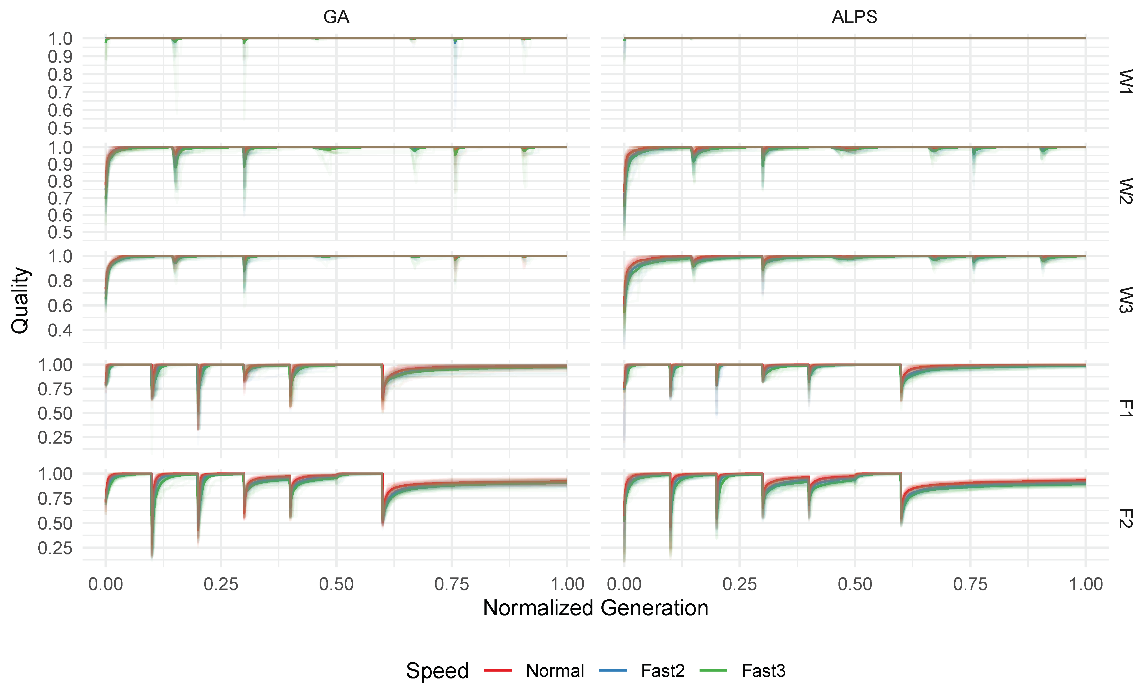
Figure 10 illustrates the quality of the best individuals for each generation under different epoch speeds (population average qualities are omitted for brevity). The results suggest that the algorithms can effectively handle increased epoch speeds, with only minimal improvements in the convergence speed and an overall better quality observed in the normal speed for some instances.

However, it is important to consider the diverse mechanisms used to introduce the epoch speedup. In the Winkler-based instances, the increased speed primarily resulted from a smaller population size, which still proved sufficient in solving the problem instance. This implies that the original configuration might be further optimized for efficiency, given that the smaller population size also performed well. For the Friedman-based instances, the number of generations passing until an epoch change was reduced, while the population size remained constant. This means that the actual time (in terms of generations) became faster, allowing the algorithm less time to adapt. This effect is particularly noticeable in the F2 instance, where faster speeds, especially Fast3, consistently lagged. We speculate that with an increasing epoch clock speed, the algorithm would face challenges in solving the problem.

In summary, increasing the epoch clock speed or decreasing the runtime budget per epoch is expected to yield similar effects. However, we did not design the experiments specifically for this comparison to validate this assumption.

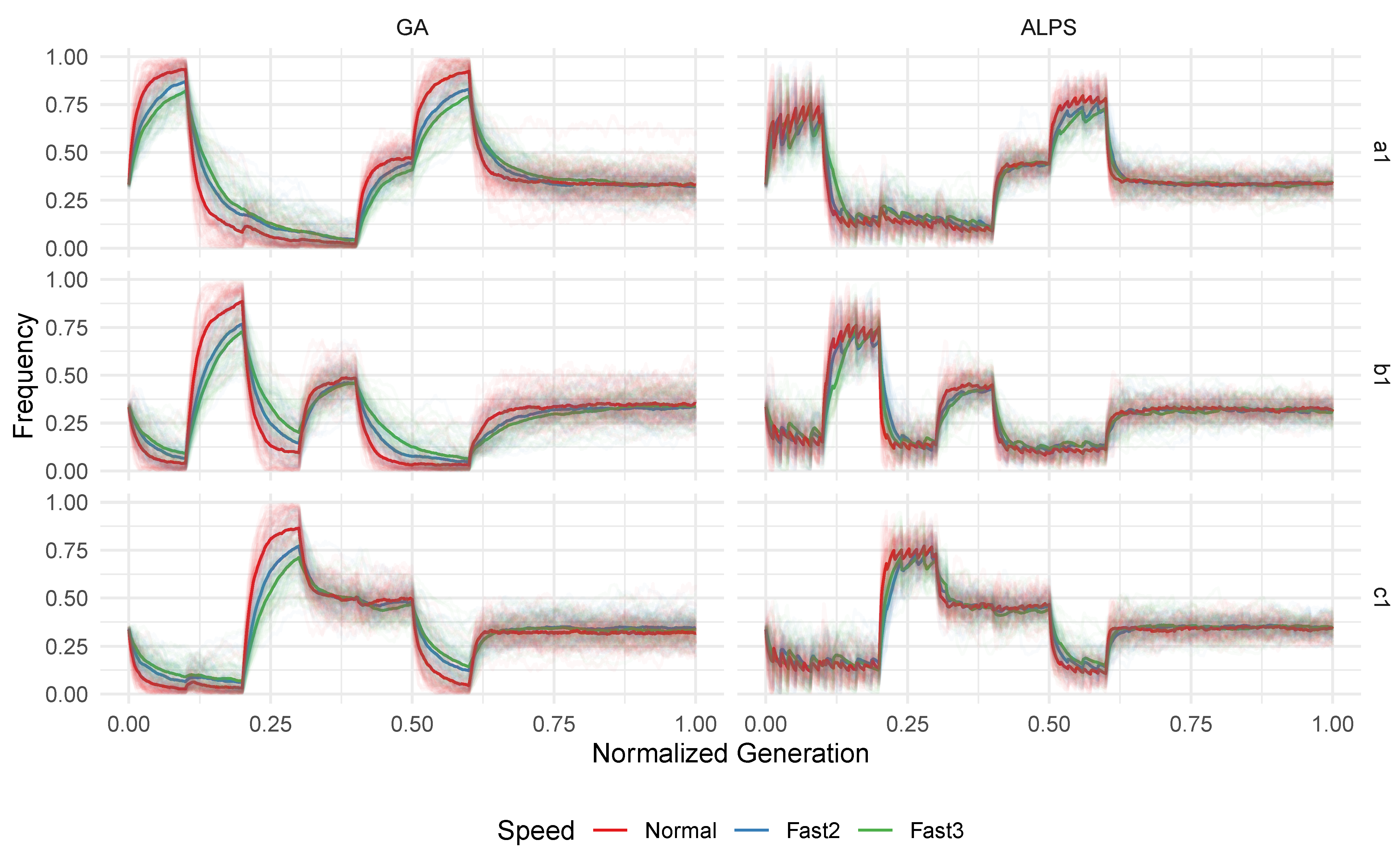
Figure 11 displays the variable frequencies across different speeds for the single instance F1 to assess the impact of the epoch speed on population adaptation. It is evident that when the epoch clock is accelerated, the variables have less time relative to the next epoch change, resulting in a slower change in frequencies. Consequently, some variables are still saturating the entire population before the next epoch occurs. This suggests that the overall diversity is higher during an epoch change, potentially benefiting GP as variables for the new epoch remain present in higher numbers in the initial population after an epoch change. This may also indicate that further acceleration of the epoch clock could lead to variables relevant for multiple epochs persisting throughout, guiding the population toward generalizing over multiple epochs. However, definitive conclusions would require additional research.

The F2 benchmark exhibits a similar pattern to F1, but the Winkler-based instances show no significant difference in variable frequencies for varying speeds, and thus these results are not included in this paper for brevity. This can be attributed to the nature of the epoch clock speed increase through a smaller population size, where the number of generations between epoch changes remains the same, allowing variables sufficient time to evolve.

The variable impacts yield similar results, with an apparent slower increase in population variable impacts for the Friedman-based instances due to faster epoch progression, while no notable differences are observed for the increased epoch speeds in the sliding window-based benchmarks, leading us to omit those results here.

3.3. Mutation Rates Results

When evaluating the impact of algorithm parameters, the usual focus is on identifying the best solution and assessing the convergence speed. However, this approach is not directly applicable to dynamic problems where multiple convergence phases and multiple best solutions occur within a single run.

Instead of solely reporting the overall best solution of individual runs, we adopt a more general analysis by examining the average quality over time. This involves calculating the mean of the best individual per generation and the mean of the average population’s quality per generation. The resulting insights into the algorithm’s overall performance across multiple epochs are illustrated in Figure 12. Lower average qualities in this context indicate suboptimal algorithm performance.

The results reveal that for the GA, mutation rates between 0.5% and 15% are effective, while the average quality drops significantly when the mutation rates are lower than 0.1%. This decline can be attributed to the fact that variables may disappear from the population and become unavailable when needed in later epochs. The GA heavily relies on mutation to maintain diversity and reintroduce lost variables. It is noteworthy that high mutation rates (5–15%) lead to a reduction in the average quality of the population. This decline is attributed to the increased disruptive impact associated with higher mutation rates.

In contrast, the ALPS leverages the reseeding mechanism as a potent tool to reintroduce lost diversity, reducing the dependence on mutation. However, it is essential to highlight that this success with the ALPS without mutation may be contingent on the application of local optimization to all numeric parameters of symbolic models using gradient descent. Without this local optimization, algorithm convergence would likely be slow or nonexistent, emphasizing the significance of mechanisms for changing numeric parameters in the absence of mutation.

As a next step, we aim to conduct a more detailed analysis of the impact of mutation rates on both the GA and ALPS. This involves focusing on a specific variable within a benchmark, closely examining the variable frequency of the population over time for each individual run. Additionally, we will distinguish cases in which a variable becomes extinct, i.e., it drops out of the population at some point. This loss of relevant building blocks and the subsequent ability to reintroduce them into the population is typically associated with mutation; therefore, we hypothesize that lower mutation rates may lead to more frequent instances of variables becoming extinct, which could explain the inferior results observed at lower mutation rates. Regarding the extinction of variables, we classify three distinct cases of extinction:

• Never: The variable is consistently present in the population at all times.
• Momentarily: The variable drops out of the population at a specific time but is later reintroduced, typically through mutation.
• Permanently: The variable drops out of the population at a specific time but is not reintroduced, remaining absent for the rest of the run.

Figure 13 shows the variable frequencies for the individual runs of variable x3 from benchmark W1 across various mutation rates. The color code indicates whether the variable was never extinct (consistently present), momentarily extinct, or permanently extinct. Please note that the entire run is color-coded based on the extinction case of the variable, rather than the specific time frame in which the extinction occurred. With very high mutation rates, variables consistently avoid extinction, as mutation continually reintroduces the variable. As mutation rates decrease, variables may experience momentary extinction, but they are regularly reintroduced through mutation. However, with very low mutation rates, as observed in the GA, variables tend to become permanently extinct more frequently. In such cases, a variable is considered irrelevant for the current epoch and may drop out of the population. The probability of mutation reintroducing it and being selected during parent selection, however, is overall too low to reliably reintroduce the variable when needed later.

For the GA, it can also be noted that as the mutation probability decreases, especially at 0.1%, the time required for reintroducing an extinct variable extends. Lower mutation rates generally extend the expected duration for the reintroduction of a variable.

Conversely, the ALPS never experiences the permanent extinction of a variable, even when momentary extinctions occur with lower mutation rates. This once again highlights the low dependence of the ALPS on mutation as a crucial genetic operator for maintaining population diversity.

An analysis of other variables and problem instances produced consistent results; however, these findings are not explicitly detailed in this paper for the sake of brevity.

4. Discussion

In the previous section, we examined the behavior of the GA and ALPS across various instances of dynamic symbolic regression problems. Our analysis focused on the overall capability of the algorithms to uncover accurate solutions (symbolic models) during the run and adapt to changes in the dataset. The results suggest that both the GA and ALPS can effectively handle dynamic changes. Following an epoch change, there is an initial dip in the average quality due to the alterations in the dataset. However, both algorithms show their adaptability to recover and to find good solutions for the modified scenario.

We also investigated the population dynamics by examining variable frequencies and variable impacts over time. The results reveal that, as anticipated, variable impacts experience an immediate drop with regime shifts in the data, while population frequency adapts more gradually in response to the changes in the fitness landscape after the change. Increases occur gradually in both variable frequencies and impacts, and these measures typically show concurrent growth. In terms of the differing behavior between the GA and ALPS, we did not observe any significant differences in this aspect. Instead, we mainly observed higher fluctuations in the measurements for the ALPS, attributable to its reseeding mechanism.

An interesting insight into population dynamics is that neither the GA nor the ALPS appear concerned with memorizing variables or subtrees for potential later use when they might become relevant again. For instance, retaining a variable that was highly relevant after an epoch change in anticipation of its future importance. While this lack of explicit memory retention was expected, creating a dedicated memory mechanism or tweaking algorithm parameters to facilitate memory functions could be explored. Options include employing a larger population size and a parent-selection mechanism with low selection pressure to prevent the loss of high-quality subtrees from past epochs. Alternatively, keeping track of parents’ old qualities from previous epochs and incorporating this past quality in the current selection of parents could be investigated. This could be achieved through a quality inheritance scheme that prioritizes offspring from parents with high quality in older epochs.

The experiments investigating faster epoch clocks suggest that, for the existing benchmarks, the available evaluation budget until the next epoch change proved to be sufficient. Consequently, the algorithms demonstrated effective adaptation to faster epoch changes. Nevertheless, we anticipate that with even faster epoch clocks, the quality at the end of an epoch would likely decrease. However, the observed drop in quality at the start of a new epoch is expected to remain comparable to that of slower epoch clocks. To effectively handle faster epoch changes, a feasible approach could be to adjust the algorithm parameters, emphasizing higher selection pressure.

In our initial findings, we consistently observed that variable frequencies rarely fell below a critical threshold. By systematically adjusting the mutation rates, we gained valuable insights into how mutation affects different algorithms. For the GA, the results show the importance of mutation in addressing dynamic problems and retaining all relevant variables in the population. Insufficient mutation rates lead to the loss of variables that may become crucial in subsequent epochs. As mutation serves as the only mechanism for reintroducing extinct variables, a low mutation rate reduces the likelihood of their reintroduction. In the absence of mutation, the GA often loses variables without the opportunity for reintroduction when needed. In contrast, the ALPS relies on its reseeding mechanism to reintroduce variables that have become extinct. Surprisingly, our results strongly suggest that the ALPS is neither sensitive to mutation rates nor reliant on mutation at all. It is essential to note that our experiments involved local optimization of numeric parameters through gradient descent, which also reduces the reliance on mutation. Without local optimization, mutation typically serves as the sole mechanism for adapting numeric parameters.

A noteworthy consideration regarding the findings of the conducted experiments is related to the definition of the benchmarks. All presented benchmarks essentially consist of weighted sums of terms, where the weights change dynamically over the epochs, and variables within the terms are exclusively used therein. This implies that the relevance of terms and their building blocks is independent of other terms. Introducing different benchmarks where terms share common subtrees or variables could alter the population dynamics. However, we suspect that having common building blocks across multiple terms might simplify the problems, as relevant building blocks could be preserved to some extent across epoch changes. Therefore, the benchmarks in this paper represent a worst-case scenario where no information carries over into another epoch for some terms.

In the conducted experiments, we exclusively employed generational epoch clocks. Using evaluation-based epoch clocks would require an adapted tuning of the algorithm parameters to achieve faster convergence up until the next epoch change.

When analyzing the performance of algorithms in dynamic environments, it showed that we currently lack a standardized approach. For instance, in comparing the overall performance in the mutation rate experiment, we resorted to simply averaging the qualities over time due to a lack of better alternatives. In contrast to static optimization problems, where standardized methods like run-length distributions and expected runtime analysis provide a statistically sound approach for analyzing performance and convergence speed [44], dynamic problems currently lack such a framework. In scenarios where epoch changes are known in advance, one could treat each epoch as an isolated run and observe run-length distributions within that epoch. This approach could yield valuable insights into algorithm performance on individual epochs. However, this method requires predefined epochs, which are often unknown in practical applications. Additionally, for gradual shifts in the data, as seen in the Winkler-based benchmarks, different considerations would be needed for analyzing such shifts.

In this study, we exclusively compared a standard genetic algorithm (GA) as a baseline with the ALPS chosen as a representative of open-ended evolutionary algorithms. Despite differences in the dependency on mutation, both algorithms yielded comparable results and demonstrated similar population dynamics. A potential direction for future research involves exploring the adaptation of alternative algorithms. For instance, an offspring-selection GA (OSGA), known for its effectiveness in non-dynamic problems, encounters challenges in dynamic scenarios, due to the offspring-selection mechanism relying on the parent qualities, which may become obsolete after an epoch change. Strategies for reevaluation post-epoch changes, akin to the reevaluation of elites in the GA and ALPS, would be essential. Exploring multi-objective algorithms, such as NSGA-II, also presents an interesting line of research. Considering the quality of previous epochs as an additional objective could motivate the algorithm to preserve valuable building blocks from past epochs.

In summary, the insights derived from this paper are not limited to symbolic regression problems alone. Various metrics exist for quantifying relevant building blocks in different problem domains, for example, relevant edges in a traveling salesman problem. Investigating the applicability of the findings in this paper to other dynamic problems is also a potential research question for the future.

5. Conclusions

This study investigated the application of genetic programming for dynamic symbolic regression, addressing challenges posed by dynamically changing training datasets. Both the genetic algorithm and Age-Layered Population Structure demonstrated notable adaptability, effectively responding to dynamic changes throughout the algorithm run.

This paper examined population dynamics, considering variable frequencies and variable impacts over time. Notably, variable frequencies exhibited a gradual shift, trailing behind variable impacts that could drop instantly when the variables were no longer relevant. Surprisingly, neither the GA nor the ALPS displayed a tendency to construct a memory for successful individuals from preceding epochs, inviting future research for refining algorithms in dynamic optimization.

Accelerating the epoch clock, the population frequency often failed to converge fully before the next epoch change. However, this did not significantly alter the algorithms’ capacity to discover good solutions, underlining their robustness in dynamic scenarios.

This study explored the role of mutation in maintaining and reintroducing genetic diversity, which is crucial in dynamic settings where variables face temporary extinction. Moderately lower mutation rates led to the momentary extinction of variables, but both the GA and ALPS mostly demonstrated resilience by reintroducing variables even with low mutation. In scenarios with minimal or no mutation, the genetic algorithm’s reliance on mutation to reintroduce variables differs from the age-layered population structure’s, which shows no significant dependence on mutation, thanks to its internal reseeding mechanism.