Featured Application
This slap-type VEH system has versatile applications, including integrating it into multi-rotor aircraft, unmanned fixed-wing aircraft, motorcycles, bicycles, and other moving objects. Additionally, it harnesses downstream flow fields from rotorcraft and fixed-wing aircraft, demonstrating the potential for green energy generation in diverse settings.
Abstract
This study introduces a groundbreaking slap-type Vibration Energy Harvesting (VEH) system, leveraging a rotating shaft with magnets to induce vibrations in an adjacent elastic steel sheet through magnetic repulsion. This unique design causes the elastic sheet to vibrate, initiating the oscillation of a seesaw-type rigid plate lever. The lever then slaps a piezoelectric patch (PZT) at the elastic steel sheet’s root, converting vibrations into electrical energy. Notably, the design enables the PZT to withstand deformation and flapping forces simultaneously, enhancing power conversion efficiency. The driving force for the rotating shaft is harnessed from the downstream flow field generated by moving objects like rotorcraft, fixed-wing aircraft, motorcycles, and bicycles. Beyond conventional vibration energy harvesting, this design taps into additional electric energy generated by the PZT’s slapping force. This study includes mathematical modeling of nonlinear elastic beams, utilizing the Method of Multiple Scales (MOMS) for in-depth vibration mode analysis. Experimental validation ensures the convergence of theory and practice, confirming the feasibility and superior voltage generation efficiency of this slap-type VEH concept compared to traditional VEH systems.
1. Introduction
Vibrations are a common occurrence in our daily lives, ranging from the vibrations of minute mechanical components to the substantial vibrations of aerospace engineering structures like airplanes and rockets. The potential to convert this energy into reusable energy holds the key to realizing sustainable management practices. With global attention increasingly focused on energy issues in recent decades, Vibration Energy Harvesting Systems (VEH) have emerged as a noteworthy green energy technology, garnering significant interest from scholars. Efficiently recycling and repurposing the constant vibrations in our surroundings could establish a robust electrical energy conversion method with substantial environmental benefits. Kim et al. [1] attribute object vibrations to factors like uneven system quality or surface irregularities resulting from material wear and tear. Pellegrini et al. [2] assert that mechanical vibration represents a dependable energy source, and its conversion to electrical energy could enable electronic devices to operate without conventional batteries. Piezoelectric devices have become a focal point in the analysis and research of power generation due to their effectiveness in converting vibration energy into electrical energy, as demonstrated by Roundy et al.’s research [3]. Moreover, piezoelectric patches (PZTs), known for their compact size and independence from additional power supplies, prove suitable for installation in various sensors, buildings, facilities, and household appliances—areas frequently subjected to tactile interactions—yielding significant energy-saving effects.
In the pursuit of compact and lightweight electronic products, Roundy and Wright [4] designed a power generation device incorporating a double-layer bendable rod and a piezoelectric patch (PZT). They anticipate that future electronic devices will trend toward smaller and lighter designs. Emphasizing the pervasive nature of vibration energy in daily life, Park et al. [5] installed a vibration energy recovery device beneath a car’s hood, utilizing natural forces such as magnets and gravity to convert vibrations into electrical energy and store it effectively.
Wu et al. [6] investigated a vibration energy harvesting system employing, during flight, piezoelectric devices installed on aircraft wings. Their study delved into the impact of different flight altitudes on aircraft vibration, underscoring the significance of aerodynamics in vibration energy recovery systems. Zhang et al. [7] devised a bistable piezoelectric energy harvester capable of recovering vibrations from general machinery, a concept gaining popularity in recent years. Rajora et al. [8] creatively utilized PZTs on simply supported beams, tapping into environmental vibrations to power small electronic devices. Khan et al. [9] proposed an innovative energy harvester employing multiple PZTs to convert vibration energy into electrical energy, storing it in an electrical storage device. Harne and Wang [10] highlighted the amplification of power generation in a bistable system during transitions between stable states, with many bistable energy harvesters employing magnetic forces for driving. Stanton et al. [11] contributed to the understanding of bistable oscillators’ power generation devices, employing magnets and cantilever beams. Their practical design considerations, including the impact of varying magnet spacing on power generation efficiency, contribute to the evolving landscape of bistable oscillator technology.
Regarding piezoelectric material technology, Kim et al. [1] have outlined that these materials typically encompass piezoelectric polycrystals, piezoelectric single crystals, and piezoelectric films. Notably, Polyvinylidene Difluoride (PVDF) stands out as a common material exhibiting a robust piezoelectric effect. Wu et al. [12] conducted an in-depth exploration of the fundamental properties, theoretical underpinnings, manufacturing techniques, and applications of piezoelectric materials. Their focus extended to the flexibility and stretchability of inorganic, polymeric, and biological piezoelectric materials, elucidating recent advancements in piezoelectronics, piezophotonics, object structures, and self-powering technologies. Recognizing the necessity for piezoelectric materials to seamlessly convert mechanical and electrical energy, Harazin and Wróbel’s research [13] delves into the stacking method employed. Their study reveals that a PZT comprises multiple piezoelectric plates with very thin dielectric material serving as a separation between layers while electrodes are connected along the sides of the PZT. In the realm of energy utilization, Resali and Salleh [14] propose the incorporation of a Power Management Circuit (PMC) to store and harness the converted electrical energy. Furthermore, Resali and their collaborators have conducted experiments aimed at minimizing the size and weight of the power management system, facilitating its integration into small mechanical equipment.
This study builds upon the findings of Wang and Chu [15] with significant enhancements. Wang and Chu [15] investigated a dual elastic steel sheet energy harvesting system, where a PZT is affixed to the free end of one elastic steel sheet, and a magnet is attached to the free end of another elastic steel sheet. Their approach involved simulating helicopter-generated downwash to induce deformation in an elastic beam with a magnet, causing it to rebound and slap a PZT on the free end of another elastic beam, thus generating electrical energy. However, the fixed-free system’s limited deformation at the free end of the elastic steel sheet constrained it to rely solely on flapping for electricity generation, preventing efficient utilization of the deformation force. In a related vein, Wang et al. [16] conducted research on a fixed-free beam system. Their designed mechanism mirrors that of Wang and Chu [15], constituting a dual elastic steel sheet energy harvesting system with components such as beams, magnets, PZTs, and rotating disks, forming a bi-stable VEH system. Like their predecessors, Wang et al. [16] positioned a PZT at the free end of one elastic steel sheet and a magnet at the free end of another elastic steel sheet. They utilized the magnet on the rotating disk to drive the magnet on the elastic beam, inducing deformation in the elastic beam. Concurrently, they harnessed the energy from the deformed elastic beam to slap the elastic beam carrying the PZT, thus generating power. Nevertheless, akin to Wang et al. [15], the PZT was primarily influenced by slapping forces, unable to fully undergo deformation due to the minimal deformation at the free end of the elastic beam. In contrast, the elastic steel sheet experienced more substantial deformation near its fixed end.
To surmount this challenge, we devised a seesaw-like mechanism illustrated in Figure 1. The slap-type VEH system concept is shown in Figure 2. As shown in Figure 2, a rotating shaft equipped with magnets is employed to induce vibrations in the adjacent elastic steel sheet through magnetic repulsion, leading to its vibration. The resulting vibrations cause the adjacent seesaw-type rigid plate lever to oscillate, slapping the PZT installed at the root of the elastic sheet. Consequently, this design facilitates the conversion of vibrational energy into electrical energy. The unique feature of this design enables the PZT to withstand both deformation and flapping forces simultaneously, resulting in superior power conversion efficiency.
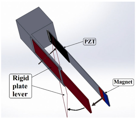
Figure 1.
Slap-type VEH system 3D mechanism diagram.
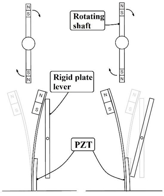
Figure 2.
Slap-type VEH system concept diagram.
In this study, the wind force can be derived from the downstream flow field generated by rotorcraft, fixed-wing aircraft, motorcycles, bicycles (see Figure 3), and other moving objects. The magneto-piezoelectric and slap-force energy harvesting device are installed onto the mechanical object. As the mechanical object advances, its relative airflow is channeled through the wind-collecting hood (also called fairing), initiating the rotation of the attached magnet’s rotating shaft (see Figure 4). The repulsive force generated by the magnet is then employed to set the fixed-free elastic steel sheet, fitted with the magnet, into vibration (refer to Figure 2). The vibrational movement of the elastic steel sheet causes its free end to impact a lever mechanism resembling a seesaw (the rigid plate lever), inducing a swinging motion. This swinging rigid plate lever, in turn, slaps the PZT installed at the root of the elastic steel sheet. This design allows the PZT to withstand both deformation and impact force simultaneously. Device schematic diagrams of slap-type VEH installed in forward and vertical flight (moving) vehicles are shown in Figure 4. Through this thoughtful design, we not only capture electrical energy through the conventional vibration energy harvesting system but also harness additional electric energy generated by the slapping force of the PZT. This approach maximizes electrical generation efficiency, ensuring the effective utilization of energy in the process.
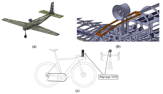
Figure 3.
Slap-type VEH applications, (a) UAV, (b) detailed construction on UAV, (c) bicycle.
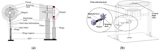
Figure 4.
Device schematic diagrams of slap-type VEH (a) installed in forward flight (moving) vehicles, (b) installed in vertical flight (moving) vehicles.
This study comprises the following sections. In Section 2, we derive the equation of motion for elastic beams, delving into an analysis of the vibration modes exhibited by the elastic steel sheet. Employing Newton’s second law, Euler’s angle transformation, and Taylor series expansions, we establish the equation for the two-dimensional nonlinear beam. In Section 3, the Method of Multiple Scales (MOMS) is utilized to examine vibrations associated with each mode, substantiating the system’s frequency response through a fixed-point plot. In Section 4, we integrate the piezoelectric equation with the nonlinear beam equation for a comprehensive assessment of theoretical electrical generation efficiency. Section 5 introduces an experimental setup to validate the accuracy of the proposed theoretical model, assessing the experimental voltage outputs for different modes. Section 6 discusses the validity of the theoretical framework, ensuring mutual confirmation between theory and practice. The feasibility of our proposed model is affirmed through this comprehensive approach. Section 7 presents the findings and conclusions derived from the study.
2. Theoretical Model
2.1. Equation of Motion
To replicate the vibration of the elastic steel sheet, we employ a nonlinear Euler-Bernoulli Beam. Drawing from Nayfeh and Pai’s theory of nonlinear beams [17], we specifically focus on the plane motion of the nonlinear beam. Employing Newton’s second law, Euler’s angle transformation, and Taylor series expansions, we derive the equation for the two-dimensional nonlinear beam as follows:
The definition of coordinates in the above equation is shown in (Figure 5). In Equations (1) and (2), represents the differential in space , denotes the differential in time , is the mass of the beam, E represents Young’s modulus, A is the cross-sectional area of the nonlinear beam, IA denotes the moment of inertia, is the uniform distributed simple harmonic load.
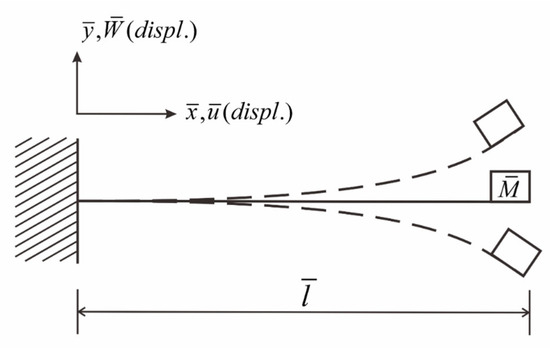
Figure 5.
Coordinate diagram of elastic beam vibration system.
We assume that the boundary conditions of this nonlinear beam are that one end is fixed, the other end is a free end, and a magnet (considered as a point mass) is added to the free end. The boundary conditions can be assumed to be:
In Equations (3)–(6), is the mass of the magnet. We assumed the free end of the system has no axial external force, and for a slender beam, the ratio of m/EA is small. The terms of are neglected. Equation (1) can be expressed as:
Equation (7) is integrated to obtain the expressions of and :
Assuming a steady deformation of , and substituting Equations (7) and (8) into Equation (2), the equation of this nonlinear beam can be simplified to the transversal direction () as follows:
where is the structural damper, represents the geometric nonlinearity, denotes the shortening effect. The dimensionless form of Equation (9) is then expressed as:
where , , , , , , represents , represents . The dimensionless boundary conditions are:
where M is the ratio of the magnet mass to the mass of the elastic steel sheet ().
2.2. Piezoelectric-Patch Equation
According to Rajora et al. [8], the piezoelectric equation for the PZT is:
The force exerted by the PZT on the nonlinear elastic beam is assumed to be the Coulomb force and can be expressed as:
where CP is the capacitance of the piezoelectric patch, and Cf represents the piezoelectric coupling coefficient. The dimensionless piezoelectric equation for the PZT can be written as:
In which , , . The dimensionless voltage output can be found using Equation (17) and is expressed as:
The dimensionless Coulomb force is written as:
In Equation (19), a and b represent the dimensionless positions of the PZT from one end to the other end and . Combining this condition with Equations (15) and (16), we obtain a dimensionless nonlinear beam equation with the PZT as:
2.3. Theoretical Model of Magnetic Equation
According to References [18,19], the expression for the potential energy caused by the repulsion between magnets can be obtained using the Biot–Savart Law:
where , is the vacuum permeability, represents the L2 Norm, is the position vector from the center of magnet B to the center of magnet, and are the magnetic moment vectors of magnets A and B, respectively, and their directions and coordinate axes are defined as shown in Figure 6 below.
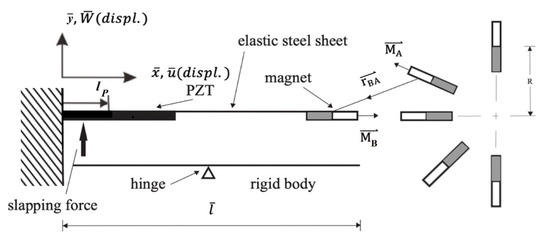
Figure 6.
Directions and coordination axes of magnets A and B.
We can obtain the Lorentz force of magnet B acting on magnet A by using the following equation:
We divide the Lorentz force of the magnet acting on the nonlinear beam by to obtain a dimensionless forcing function (FM). Subsequently, let dRs = , MVc = , WRc = and MVs = . The magnetic force FM can be expressed as,
In this context, MA and MB denote the magnetic moments of magnets A and B; VA and VB represent the volumes of magnets A and B, respectively. The variable d signifies the distance between magnets A and B, while α denotes the angle of magnet A, and R indicates the rotation radius of magnet A. By incorporating the dimensionless magnetic force function (23) into the Equation (20) governing the piezoelectric nonlinear beam, the resulting equation for the magneto-electric VEH system is as follows:
2.4. Method of Multiple Scales, MOMS
We employed the Method of Multiple Scales (MOMS) to analyze nonlinear equations. The MOMS divides the time into two scales: fast time change and slow time change. In this context, the term with fast time change is denoted as , and the term with slow time change is denoted as , with representing the time scale of small disturbance. Assuming , Equation (24) can be derived:
In Equation (25), is considered an extreme, small value, and we thus neglect the impact of higher-order terms, such as etc., on the overall system. The terms composed of order are then expressed as:
The terms composed of order are then expressed as:
3. Frequency Response
We employed the method of separation of variables to decompose W0 into time and spatial domain, defining it as:
By substituting Equation (28) into Equation (26) and incorporating the boundary conditions, we derived the characteristic equation:
where α represents the system eigenvalue. The mode shape can then be expressed as:
Then, the general solution of can be expressed in terms of mode shape and generalized coordinate as follows:
where , is the phase angle, and Bn represents the amplitude of the nth mode. Substituting Equations (31) and (32) into Equations (26) and (27) and then using orthogonal property, the following equation can be obtained:
Order of :
Order of :
where Qm represents . By examining Equations (33) and (34), it becomes apparent that the term involves the interplay of modes within this beam. Consequently, we will delve into the analysis of coupling effects among the first three modes of this elastic beam. When considering the frequency response of the system, the external force can be expressed as the following function:
where and is the tuned frequency. When considering the excitation of the first mode (m = 1) and selecting all terms containing , i.e., secular terms, Equation (27) can be expressed as:
where represents the slapping position on the PZT. Similarly, when exciting the second mode (m = 2), we select all terms containing . The same process is applied when exciting the third mode (m = 3), where all terms containing are chosen. This allows us to derive the secular terms for each mode. By setting the sum of the secular terms to zero, we establish the solvability condition for each mode. Subsequently, we can generate a fixed-point plot to analyze the frequency response of the system.
We multiply Equation (36) for the secular terms of the first mode by and let . Assuming that when the frequency response is in a steady state (, ), we obtain and . The solvability condition of Equation (36) is then separated into real and imaginary parts. The real part equation for the first mode is expressed as follows:
The imaginary part equation for the first mode is expressed as follows:
We square sum Equations (37) and (38) to eliminate the time-related terms (). The resulting equation becomes:
Similarly, multiplying the secular terms for the second mode by and the secular terms for the third mode by , we obtain the equations for the real and imaginary parts of the second and third modes. Utilizing the IMSL subroutine “NEQNF”, employing the Levenberg-Marquardt method, allows us to solve the solvability conditions. Consequently, we can derive the dimensionless amplitudes B1, B2, and B3 for this system and generate tuned-frequency response diagrams for each mode, known as fixed-point plots. Applying the same approach, we can obtain tuned-frequency response diagrams for the second and third modes. Figure 7 represents the fixed-point plots for the first, second, and third modes when the first mode is excited. Figure 8 depicts the fixed-point plots for the second mode when the second mode is excited. Figure 9 illustrates the fixed-point plots for the first, second, and third modes when the third mode is excited. Notably, Figure 7 demonstrates that when the first mode is excited, the amplitude of the first mode significantly surpasses that of the second and third modes. This observation is consistent with other modes.
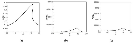
Figure 7.
Fixed-point plot when exciting the 1st mode, (a) the 1st mode plot, (b) the 2nd mode plot, (c) the 3rd mode plot.
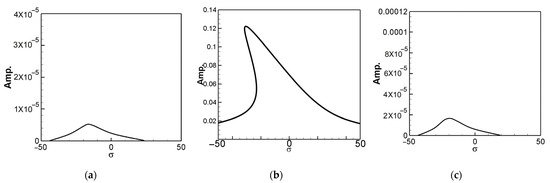
Figure 8.
Fixed-point plot when exciting the 2nd mode, (a) the 1st mode plot, (b) the 2nd mode plot, (c) the 3rd mode plot.
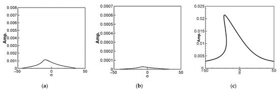
Figure 9.
Fixed-point plot when exciting the 3rd mode, (a) the 1st mode plot, (b) the 2nd mode plot, (c) the 3rd mode plot.
4. Voltage Generation Benefit Analysis
We use the fourth-order Runge–Kutta method and the small perturbation method to find the theoretical voltage of this system. The theoretical model of the slapping force on the PZT at the root of the elastic steel sheet and the overall voltage generation equation is constructed as follows.
We assume that the impact force of the rigid plate lever slapping the PZT is regarded as:
where is the slapping period and denotes the Dirac function.
Divide Equation (40) by to obtain the dimensionless slapping force: . Then add Equation (40) to Equation (24) to obtain the dimensionless nonlinear beam equation with the slapping force as follows:
Apply the small perturbation method by assuming to be , where denotes the equilibrium periodic term and represents the perturbation term. After substituting and into Equation (41) and orthogonalizing it, the resulting equation is as follows:
Next, we solved Equation (42) using the fourth-order Runge–Kutta method and generated time response plots for the first, second, and third modes (refer to Figure 10). By comparing the displacements of the time response plots and the amplitudes of the fixed-point plots, the accuracy of the fixed-point plots can be confirmed.
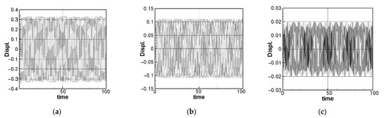
Figure 10.
Time response plots, (a) the 1st mode, (b) the 2nd mode, (c) the 3rd mode.
The amplitude for each mode can be identified utilizing information from the fixed-point plots. This data is then applied to Equations (42) and (18), and the theoretical voltage generation diagram is computed using the fourth-order Runge–Kutta method. Figure 11 illustrates the theoretical voltage diagrams for the first, second, and third modes when the PZT is placed at the root of the elastic steel sheet.
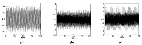
Figure 11.
The theoretical voltage outputs (a) the 1st mode, (b) the 2nd mode, (c) the 3rd mode.
Subsequently, we introduced a mass to the slapping end of the lever structure, aiming to enhance the efficiency of voltage generation by slapping the PZT. Various masses were incorporated into the slapping force term of the equation. Figure 12a–e illustrate the theoretical voltage generation diagrams for the first mode with additional masses of 1 g, 3 g, 5 g, 7 g, and 9 g, respectively. In Figure 13, the impact of an adding mass of 5 g on voltage generation efficiency becomes evident. Consequently, in forthcoming experiments, we plan to append a mass to the end of the lever structure responsible for striking the piezoelectric patch. Furthermore, a resistance will be introduced for analysis, with the objective of calculating the optimal electrical power output of the system.
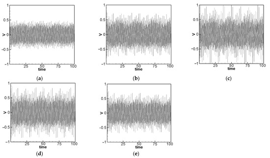
Figure 12.
Theoretical voltage outputs of the 1st mode for different masses added to the lever end: (a) 1 g, (b) 3 g, (c) 5 g, (d) 7 g, (e) 9 g.
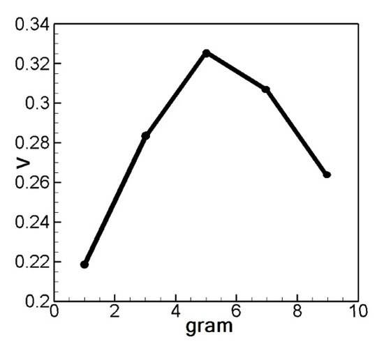
Figure 13.
Comparison chart of added masses (in g) and voltage.
5. Experimental Setup and Verification Analysis
5.1. Experimental Setup
We utilized a brushless motor, specifically the 5008-335KV model, along with carbon fiber rotor propellers and a wind collecting hood to construct a setup that emulates the downwash generated by a helicopter or other rotorcraft during operation (refer to Figure 14). This assembly was affixed to an optical table. We incorporated a wind turbine rotor shaft with a 45 mm rotation radius and attached magnets beneath the wind collecting hood, as illustrated in Figure 15. The configuration of the slap-type VEH is shown in Figure 16. The electric generation mechanism was securely mounted on a metal rod. As the downwash is generated and flows through the rotating wind turbine, causing the rotating shaft to rotate, the magnets attached to the rotating shaft induce changes in the magnetic field within the system. Subsequently, these alterations in the magnetic field are utilized to excite the elastic steel sheet, leading to its deformation and striking of the rigid plate lever. Once the lever is stimulated, it, in turn, slaps the piezoelectric patch positioned at the root of the elastic steel sheet, causing the PZT to deform and generate electricity.

Figure 14.
Wind collecting hood with a vertical flight rotor.
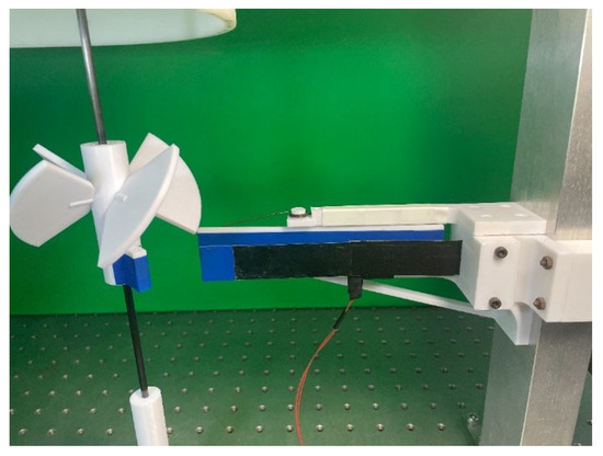
Figure 15.
Rotor shaft with magnets beneath the wind collecting hood and the slap-type VEH.
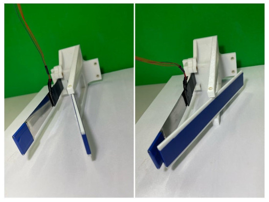
Figure 16.
Configuration of the slap-type VEH.
5.2. Natural Frequency Measurement
To validate the accuracy of the natural frequency analysis, it is essential to measure the natural frequency of the elastic steel sheet with an attached magnet within the experimental system. We employed an impact hammer (model 2302, Meggitt, UK) and an accelerometer, which are connected to the imc© (CS-5008-1, TÜV Rheinland, Kölle, Germany) data processor for analysis. Our findings indicate that the natural vibration frequencies of the first three modes of the elastic steel sheet with the attached magnet are 4.56 Hz, 21.48 Hz, and 60.06 Hz, respectively (see Figure 17). After the numerical calculation of Equation (29), the first three eigenvalues can be obtained: 2.1264, 4.7142, and 7.8590. The theoretical dimensional frequencies for the first three modes are 4.5216 Hz, 22.2237 Hz, and 61.7639 Hz, respectively.
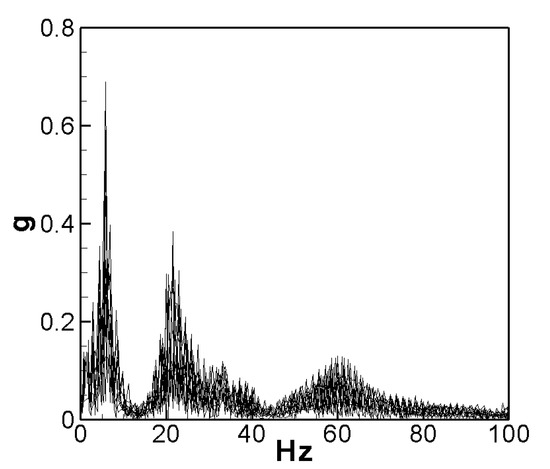
Figure 17.
Natural frequencies of the first three modes.
5.3. System Resistance Measurement
To assess the electrical power of this slap-type wind-driven power generation system, we introduced a resistance into the system as a load. The optimal electrical power is achieved when the added resistance value closely matches the internal resistance of the system. Following Thevenin’s theorem, the internal resistance value of this system can be determined with the following equation:
where VL is the voltage, RL denotes resistance, RT represents the internal resistance, VT is the open-circuit voltage. The electric power equation is written as:
where P is the power, V represents the voltage, I denotes the current, and R is the resistance. After combining Equations (43) and (44), the following equation can be obtained:
Equation (45) reveals that the optimal electrical power can be attained when the load resistance (RL) is equal to the internal resistance (RT) of the system. We conducted experiments to investigate the impact of adding mass to the end of the rigid flat plate lever responsible for slapping the PZT. Specifically, we introduced a mass of 1 g to the lever end for experimental analysis. We employed an imc© data processor to measure the open-circuit voltage of the system, conducting five measurements to ensure data reliability. The average voltage obtained from these experiments was 4.846 volts. Subsequently, we introduced a 30 K-ohm resistance device into the system, conducting five additional experiments to ensure data consistency. The average voltage measured with the 30 K-ohm resistance was 1.735 volts. By incorporating the average open-circuit voltage and the average voltage obtained with the 30 K-ohm resistance into Equation (43), the theoretical value of the internal resistance of the system was calculated to be approximately 53,802 ohms (rounded to 54 K ohms). In the subsequent step, we tested and added resistances of 44 K, 49 K, 54 K, 59 K, and 64 K ohms as load resistances, recording the corresponding voltage and electric power as presented in Table 1. Utilizing the data from Table 1, we generated the ohms-volts and ohms-power diagrams (refer to Figure 18 and Figure 19). It is evident from Table 1 and Figure 19 that when the attached resistance is 54 K, the system achieves its highest output power of 0.12056 mW.

Table 1.
Corresponding voltage and power for different resistances of 1 g mass added to the lever end.
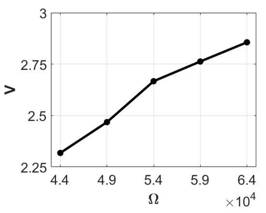
Figure 18.
Ohms-volts diagram with 1 g.
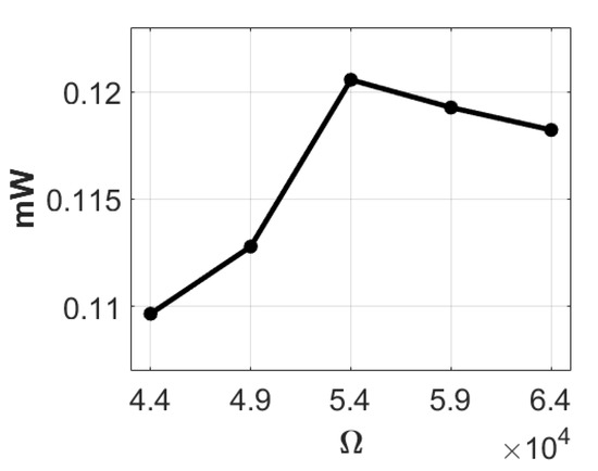
Figure 19.
Ohms-power diagram with 1 g.
Next, we introduced masses of 3 g, 5 g, and 7 g to the lever end for experimental analysis. Employing the imc© data processor, we measured the open-circuit voltage of the system with a 3-g mass added to the end of the lever. After five experiments, the average measured voltage was 6.027 volts. Subsequently, a 30 K-ohm resistance was incorporated into the system, and after five additional experiments, the average voltage with the resistance was recorded as 2.132 volts. By averaging the open-circuit voltage and the resistance-added voltage and incorporating these values into Equation (43), the theoretical internal resistance of the system was calculated to be approximately 54,801 ohms (rounded to 55 K ohms). In the subsequent step, we tested the system with resistances of 45 K, 50 K, 55 K, 60 K, and 65 K ohms, recording the corresponding voltage and electric power as shown in Table 2. Utilizing this data, we plotted the ohm-volt and ohm-electric power diagrams (Figure 20 and Figure 21). Analysis of Table 2 and Figure 21 reveals that when the attached resistance is 55 K, the system achieves its highest output power at 0.161765483 mW.
Table 2.
Corresponding voltage and power for different resistances of 3 g mass added to the lever end.
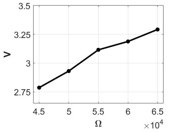
Figure 20.
Ohms-volts diagram with 3 g.
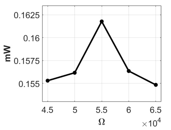
Figure 21.
Ohms-power diagram with 3 g.
Continuing the experiments, we added a 5-g mass to the end of the lever element slapping the piezoelectric patch, measuring the open-circuit voltage of the system. After five experiments, the average voltage was found to be 5.783 volts. Five additional experiments yielded an average voltage of 2.064 volts, using a 30 K-ohm resistance as the load resistance in the system. By substituting the average voltage into Equation (43), the theoretical internal resistance of the system was calculated to be approximately 54,043 ohms (rounded to 54 K ohms). We then tested the system with resistances of 44 K, 49 K, 54 K, 59 K, and 64 K ohms, recording the corresponding voltage and electric power as shown in Table 3. Using this data, we plotted the ohm-volt and ohm-electric power diagrams (Figure 22 and Figure 23). Analysis of Table 3 and Figure 23 reveals that when the attached resistance is 54 K, the system achieves its highest output power at 0.179359314 mW.
Table 3.
Corresponding voltage and power for different resistances of 5 g mass added to the lever end.
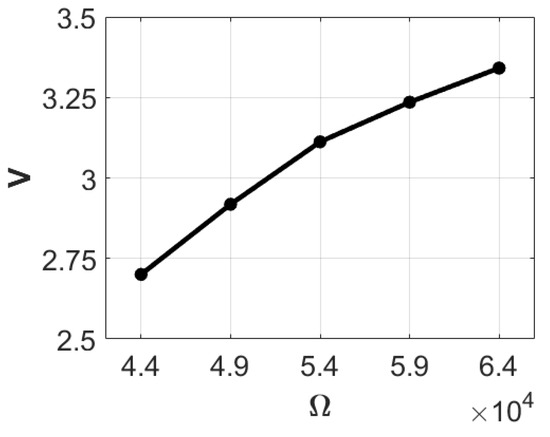
Figure 22.
Ohms-volts diagram with 5 g.
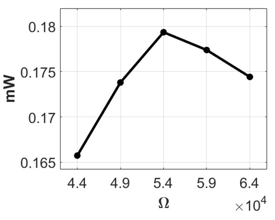
Figure 23.
Ohms-power diagram with 5 g.
Finally, we introduced a 7-g mass block to the end of the lever and carried out five trials. The average measured voltage in these experiments was 5.737 volts. The theoretical value of the internal resistance of the system was calculated to be 54,550 ohms (rounded to 55 K ohms). Employing load resistances of 30 K, 45 K, 50 K, 55 K, 60 K, and 65 K ohms, we calculated the corresponding voltage and electric power as presented in Table 4. Figure 24 and Figure 25 depict their respective ohm-volt and ohm-electric power diagrams. It is evident from Table 4 and Figure 25 that when the load resistance is 55 K, the system attains its highest output electric power at 0.167406107 mW.
Table 4.
Corresponding voltage and power for different resistances of 7 g mass added to the lever end.
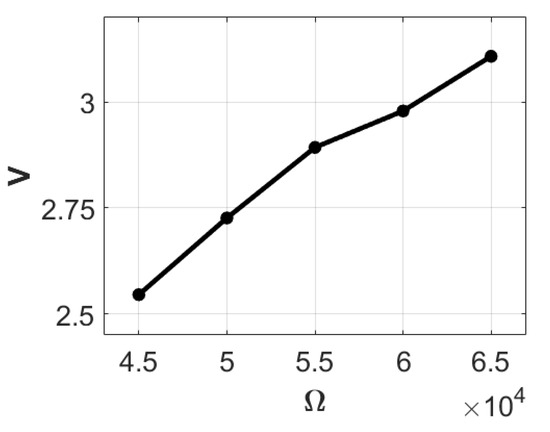
Figure 24.
Ohms-volts diagram with 7 g.
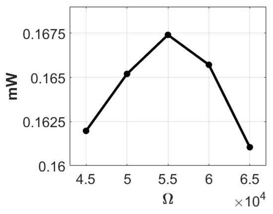
Figure 25.
Ohms-power diagram with 7 g.
Based on the experimental data above, the calculated internal resistance values obtained through open-circuit voltage and load voltage in the four sets of experiments are 53,802, 54,043, 54,550, and 54,801 ohms, respectively. Considering the results of the internal resistance measurement experiment, the configuration yielding superior power generation efficiency involves adding a 5-g mass block at the end of the lever and using a 54 K-ohm resistance as the load resistance. Therefore, this specific combination will be employed for experiments in the subsequent Sections.
5.4. Voltage Measurement
By analyzing the natural frequency of the system, it can be deduced that when exciting the first three modes, the revolutions per minute (RPM) of the rotating shaft are approximately 175 RPM, 645 RPM, and 1800 RPM, respectively. After establishing the rotating shaft speeds for the first three excitation modes and introducing a 5-g mass to the end of the lever with a 54 K-ohm resistance as the load resistance, the voltage of the root-slapping wind-driven power generation system is determined through experimental testing. Following the experiment, the output voltages for the first three modes were measured, as shown in Figure 26. The results obtained from five experiments are summarized in Table 5. Examining the voltage diagrams for the first three modes reveals an increase in power generation voltage with each successive mode. This increase in output volts aligns with the trend predicted through theoretical voltage projections. To emphasize the practical applicability of this model, this study presents cumulative measurements of the energy collected over a specific period of time, allowing the reader to gain a comprehensive understanding of the system’s performance. We summarize the power generation and voltage output data for 60 s in the experiment in Table 5. The last two rows of Table 5 show the overall harvested energy, providing a comprehensive reference emphasizing the practical application of the model.
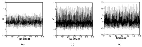
Figure 26.
Experimental voltage output: (a) the 1st mode was excited, (b) the 2nd mode was excited, (c) the 3rd mode was excited.
Table 5.
Experimental voltage and power output of the first three modes.
6. Discussion of Theoretical and Experimental Results
Table 5 reveals that the average root mean square voltage of the first three modes are 1.726, 2.184, and 2.229 volts, yielding a ratio of 1:1.265:1.291. Following dimension conversion, the root means square voltage values predicted by theory for the first three modes are displayed in Figure 27, measuring 1.773 volts, 2.282 volts, and 6.658 volts, respectively. The relative errors between the theoretical and experimental voltage outputs are approximately 2.717%, 4.497%, and 198.688%, respectively. The theoretical voltage output ratio for the first three modes is 1:1.287:3.755. From the results, it is evident that the experimental data for the first and second modes align well with the theoretically predicted values. However, discrepancies in the third mode may be attributed to the inability of the magnet at the free end of the elastic steel sheet to synchronize with the frequency of the magnet on the rotating shaft. Consequently, irregular motion in the slapping of the elastic steel sheet and the lever led to a mismatch between the third mode voltage output and the theoretical value.
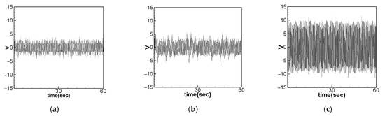
Figure 27.
Theoretical voltage output: (a) the 1st mode was excited, (b) the 2nd mode was excited, (c) the 3rd mode was excited.
To verify that the power generation efficiency of the system improves with the addition of slapping force compared to without, we conducted theoretical and experimental analyses on the first and second modes of the system without the addition of slapping force. As irregular motion was observed in the third mode, we have excluded it from further discussion. The theoretical considerations and root mean square data from five experiments for the first and second modes without slapping the root are presented in Table 6. The theoretical and experimental voltage diagrams for the system are illustrated in Figure 28 and Figure 29. An analysis of Table 6 and Figure 28 and Figure 29 reveals that the theoretical and experimental errors for the first and second modes without adding slap force fall within 10%. A comparison of voltage root means square values with and without slapping force in Table 7 indicates a significant increase in generated volts when slapping force is applied. To underscore the practical applicability of this model, this study also summarizes the power generation and voltage output data for 60 s in the experiment in Table 7. Consequently, it can be confirmed that applying slapping force on the piezoelectric sheet enhances voltage generation efficiency.
Table 6.
Theoretical and experimental voltage outputs without slapping force.
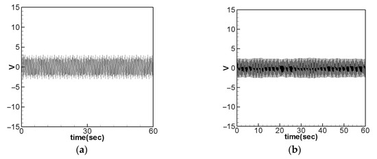
Figure 28.
Voltage output without slapping force when the 1st mode was excited, (a) theoretical prediction, (b) experimental data.
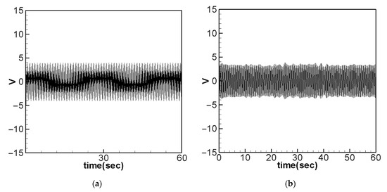
Figure 29.
Voltage output without slapping force when the 2nd mode was excited, (a) theoretical prediction, (b) experimental data.
Table 7.
Theoretical and experimental voltage outputs with/without slapping force.
In summary, this fundamental slap-type wind-driven power generation system effectively enables piezoelectric patches to generate electricity through deformation and slapping forces. In the past, most PZTs only utilized either deformation to generate electricity. Therefore, we believe that this innovative approach holds great promise for the future.
7. Conclusions
This study employed a nonlinear elastic cantilever beam as the primary structure, scrutinized its vibration modes for energy harvesting, and employed Newton’s second law, Euler’s angle transformation, and Taylor series expansions to derive the equation of the nonlinear beam. By incorporating the piezoelectric equation, magnet repulsion, and lever-type single-point slapping force, the coupling equation for this system was established. The Method of Multiple Scales (MOMS) was used to analyze the frequency response, and fixed-point plots were made to ascertain the occurrence of internal resonance. The output voltage of the PZT subjected to the slap force was simulated using the fourth-order Runge–Kutta method. Finally, the validity of the theoretical framework was confirmed through experiments, leading to the following conclusions regarding this foundational slap-type wind-driven power generation system:
- Utilizing Thevenin’s theorem and experimental outcomes, it is determined that with an internal resistance of 54,000 ohms and the addition of a 5-g mass to the lever’s end, this power generation system attains its highest output electrical power.
- The experimental data and theoretical power generation voltage analysis indicate an increasing output voltage with increasing mode.
- Comparing the experimental data and theoretical root mean square voltage values for voltage generation, the first and second modes align closely with theoretical predictions. However, the irregular vibration of the elastic steel sheet in the third mode is attributed to a mismatch between the changing frequency of the rotating magnetic field from the attached magnet on the rotating shaft and the elastic steel sheet, preventing it from reaching the theoretical voltage.
- This study confirms that the slap-type VEH concept is feasible and has better voltage generation efficiency than the traditional VEH system without slapping force.
In conclusion, experiments have validated the feasibility of utilizing deformation and flapping forces on a PZT to generate electricity simultaneously. The results affirm its capability for electricity generation. The prospect is promising for commercializing such power generation systems, envisioning installations on various platforms like multi-rotor aircraft, unmanned fixed-wing aircraft, motorcycles, or bicycles. Moreover, harnessing previously overlooked waste energy in downstream flow fields for electrical generation holds significant potential. By transforming waste into a valuable resource, this approach contributes to environmental preservation.
Author Contributions
Conceptualization, methodology, validation, formal analysis, investigation, writing—original draft preparation, Y.-R.W.; analysis, investigation, visualization, experiments, J.-W.C. analysis, investigation, experiments, writing, C.-Y.L. All authors have read and agreed to the published version of the manuscript.
Funding
This research was supported by the National Science and Technology Council of Taiwan, Republic of China (grant number: NSTC 112-2221-E-032-042).
Institutional Review Board Statement
Not applicable.
Informed Consent Statement
Not applicable.
Data Availability Statement
The experimental measurement model of this study can be found at the following link: https://www.youtube.com/shorts/ncf30hAp4Yc (accessed on 2 January 2024). Its application in multi-axis unmanned rotorcraft can be found at the following link: https://www.youtube.com/watch?v=Edo97suyfnM&ab_channel=JeevanChang (accessed on 2 January 2024).
Conflicts of Interest
The authors declare no conflicts of interest.
References
- Kim, H.; Tadesse, Y.; Priya, S. Piezoelectric Energy Harvesting. In Energy Harvesting Technologies; Springer: Boston, MA, USA, 2009; pp. 3–39. [Google Scholar] [CrossRef]
- Pellegrini, S.P.; Tolou, N.; Schenk, M.; Herder, J.L. Bistable vibration energy harvesters: A review. J. Intell. Mater. Syst. Struct. 2013, 24, 1303–1312. [Google Scholar] [CrossRef]
- Roundy, S.; Wright, P.K.; Rabaey, J. A study of low-level vibrations as a power source for wireless sensor nodes. Comput. Commun. 2003, 26, 1131–1144. [Google Scholar] [CrossRef]
- Roundy, S.; Wright, P.K. A piezoelectric vibration-based generator for wireless electronics. Smart Mater. Struct. 2004, 13, 1131–1142. [Google Scholar] [CrossRef]
- Park, M.; Cho, S.; Yun, Y.; La, M.; Park, S.J.; Choi, D. A highly sensitive magnetic configuration-based triboelectric nanogenerator for multidirectional vibration energy harvesting and self-powered environmental monitoring. Int. J. Energy Res. 2021, 45, 18262–18274. [Google Scholar] [CrossRef]
- Wu, Y.; Li, D.; Xiang, J. On the energy harvesting potential of an airfoil-based piezoaeroelastic harvester from coupled pitch-plunge-lead-lag vibrations. In Proceedings of the AIAA SciTech Forum, Grapevine, TX, USA, 9–13 January 2017. AIAA 2017-0629. [Google Scholar]
- Zhang, X.; Tian, H.; Pan, J.; Chen, X.; Huang, M.; Xu, H.; Zhu, F.; Guo, Y. Vibration Characteristics and Experimental Research of an Improved Bistable Piezoelectric Energy Harvester. Appl. Sci. 2023, 13, 258. [Google Scholar] [CrossRef]
- Rajora, A.; Dwivedi, A.; Vyas, A.; Gupta, S.; Tyagi, A. Energy Harvesting Estimation from the Vibration of a Simply Supported Beam. Int. J. Acoust. Vib. 2017, 22, 186–193. [Google Scholar] [CrossRef]
- Khan, M.B.; Saif, H.; Lee, K.; Lee, Y. Dual Piezoelectric Energy Investing and Harvesting Interface for High-Voltage Input. Sensors 2021, 21, 2357. [Google Scholar] [CrossRef] [PubMed]
- Harne, R.L.; Wang, K.W. A review of the recent research on vibration energy harvesting via bistable systems. Smart Mater. Struct. 2013, 22, 023001. [Google Scholar] [CrossRef]
- Stanton, S.C.; McGehee, C.C.; Mann, B.P. Nonlinear dynamics for broadband energy harvesting: Investigation of a bistable piezoelectric inertial generator. Phys. D 2010, 239, 640–653. [Google Scholar] [CrossRef]
- Wu, Y.; Ma, Y.; Zheng, H.; Ramakrishna, S. Piezoelectric materials for flexible and wearable electronics: A review. Mater. Des. 2021, 211, 110164. [Google Scholar] [CrossRef]
- Harazin, J.; Wróbel, A. Empirical analysis of piezoelectric stacks composed of plates with different parameters and excited with different frequencies. IOP Conf. Ser. Mater. Sci. Eng. 2022, 1239, 012008. [Google Scholar] [CrossRef]
- Mohd Resali, M.S.; Salleh, H. Development of Multiple-Input Power Management Circuit for Piezoelectric Harvester. J. Mech. Eng. 2017, 2, 215–230. [Google Scholar]
- Wang, Y.R.; Chu, M.C. Analysis of Double Elastic Steel Wind Driven Magneto-Electric Vibration Energy Harvesting System. Sensors 2021, 21, 7364. [Google Scholar] [CrossRef] [PubMed]
- Wang, Y.R.; Feng, C.K.; Cheng, C.H.; Chen, P.T. Analysis of a Clapping Vibration Energy Harvesting System in a Rotating Magnetic Field. Sensors 2022, 22, 6916. [Google Scholar] [CrossRef] [PubMed]
- Nayfeh, A.H.; Pai, P.F. Linear and Nonlinear Structural Mechanics; Wiley-Interscience: New York, NY, USA, 2004; Chapters 4 and 5. [Google Scholar]
- Leng, Y.-G.; Gao, Y.-J.; Tan, D.; Fan, S.B.; Lai, Z.H. An elastic-support model for enhanced bistable piezoelectric energy harvesting from random vibrations. J. Appl. Phys. 2015, 117, 64901. [Google Scholar] [CrossRef]
- Wang, Y.-R.; Chen, P.-T. Energy harvesting analysis of the magneto-electric and fluid-structure interaction parametric excited system. J. Sound Vib. 2024, 569, 118087. [Google Scholar] [CrossRef]
Disclaimer/Publisher’s Note: The statements, opinions and data contained in all publications are solely those of the individual author(s) and contributor(s) and not of MDPI and/or the editor(s). MDPI and/or the editor(s) disclaim responsibility for any injury to people or property resulting from any ideas, methods, instructions or products referred to in the content. |
© 2024 by the authors. Licensee MDPI, Basel, Switzerland. This article is an open access article distributed under the terms and conditions of the Creative Commons Attribution (CC BY) license (https://creativecommons.org/licenses/by/4.0/).