Article

MTC-GAN Bearing Fault Diagnosis for Small Samples and Variable Operating Conditions

College of Mechanical Engineering, Shenyang Ligong University, Nanping Middle Road 6, Shenyang 110159, China
*
Author to whom correspondence should be addressed.
Appl. Sci. 2024, 14(19), 8791; https://doi.org/10.3390/app14198791
Submission received: 17 August 2024 / Revised: 17 September 2024 / Accepted: 25 September 2024 / Published: 29 September 2024

Abstract

:
In response to the challenges of bearing fault diagnosis under small sample sizes and variable operating conditions, this paper proposes a novel method based on the two-dimensional analysis of vibration acceleration signals and a Multi-Task Conditional Generative Adversarial Network (MTC-GAN). This method first constructs two-dimensional images of vibration signals by leveraging the physical properties of the bearing acceleration signals and employs Local Binary Patterns (LBP) to extract subtle texture features from these images, thereby generating fault feature signatures with high discriminative power across different operating conditions. Subsequently, MTC-GAN is utilized for data augmentation, and the trained discriminator is used to perform fault classification tasks, improving classification accuracy under conditions with small sample sizes. Experimental results demonstrate that the proposed method achieves excellent fault diagnosis accuracy and robustness under both small sample sizes and varying operating conditions. Compared to traditional methods, this approach exhibits higher efficiency and reliability in handling complex operating conditions and data scarcity.

1. Introduction

Bearings are core rotating parts widely used in various types of mechanical equipment. Their state of health is directly related to the reliability and safety of the entire system. For example, in the field of wind power generation, the reliability of bearings directly affects power generation efficiency and maintenance costs; in the automotive industry, the performance of bearings determines the smoothness of vehicle operation and the safety of passengers. Therefore, accurate bearing fault diagnosis techniques are of great significance for ensuring continuous equipment operation and reducing unplanned downtime [1,2].
Most traditional bearing fault diagnosis methods are based on specific operating conditions and sufficient sample data. These methods typically rely on a large amount of historical data collected under specific operating conditions and identify fault characteristics through statistical analysis, spectral analysis, or physical model-based analysis. However, in practice, bearings are often subjected to variable operating conditions, such as changing loads, speeds, or ambient temperatures. These variations significantly affect the operating conditions and fault characteristics of the bearings, making fault diagnosis more complex. Additionally, due to the random and unpredictable nature of bearing failures, early failures are often difficult to accurately capture with traditional monitoring methods. This is especially true in the early stages when collecting fault data is particularly challenging, leading to insufficient data in practical applications. Variable operating conditions and insufficient data together constitute two major challenges in bearing fault diagnosis research.
Many scholars have conducted related research on variable operating conditions. Zhang et al. [3] proposed an open set domain adaptive adversarial network framework for bearing fault diagnosis under multiple operating conditions. Their study emphasized the problem of negative migration due to unknown fault samples in the target domain. They effectively addressed this challenge by estimating the similarity of each target domain sample with the known categories in the source domain. Wang et al. [4] proposed an improved adversarial migration network for bearing fault diagnosis under variable operating conditions. This study optimized the feature fusion and domain migration learning performance of the network by combining the short-time Fourier transform and a channel attention module. Wang et al. [4] also proposed an improved adversarial migration network that integrates the short-time Fourier transform and a channel attention module for bearing fault diagnosis under different operating conditions. The method was validated on several datasets. Lourari et al. [5] proposed a bearing fault diagnosis method based on complete ensemble empirical modal decomposition and sequential backward selection, combining vibration and electrical signals to improve the accuracy of fault diagnosis under variable operating conditions. Chen et al. [6] proposed a semi-supervised learning-based method to address the problem of bearing fault diagnosis under variable operating conditions and unbalanced unlabeled data. Their method effectively utilizes rich unlabeled samples and improves diagnostic accuracy through the Graph Rebalancing Semi-Supervised Learning (GRSSL) algorithm. Jin et al. [7] introduced a bearing fault diagnosis method based on a Regularized Domain Adaptive Deep Neural Network (RDADNN), which maintains data distribution consistency under variable operating conditions and improves diagnostic accuracy. Lourari et al. [5] introduced a method combining complete ensemble empirical modal decomposition (CEEMDAN) and sequential backward selection (SBS) for bearing fault diagnosis under variable operating conditions, incorporating both vibration and electrical signals to verify its effectiveness.
For the small sample problem, many scholars have conducted related research. Peng et al. [8] used Conditional Deep Convolutional Adversarial Generative Networks (C-DCGAN) to address the issue of insufficient and uneven sample distribution. They improved the generative network’s structure and adopted the Wasserstein distance as the loss function, effectively enhancing fault classification on small sample datasets. Pan et al. [9] developed a semi-supervised adversarial migration network for cross-domain intelligent fault diagnosis of bearings, introducing the Gramian Angular Field to convert time-domain vibration signals into images, and designed a dynamic adversarial migration network to extract domain-invariant features from these signal images. Di Maggio et al. [10] applied a zero-shot generative AI technique based on recurrent consistent adversarial networks to synthesize highly realistic training data, thus improving transfer learning effectiveness for convolutional neural networks. Ruan et al. [11] reviewed the advancements in Generative Adversarial Networks (GAN) for bearing fault diagnosis, particularly highlighting improvements in GAN structures and loss functions, which have proven effective in addressing the issues of small sample sizes and dataset imbalance. Wang et al. [4] introduced a novel framework for bearing fault diagnosis that integrates digital twin data with transfer learning theory to address the challenge of limited fault data in industrial applications. Similarly, Wang et al. [4] used GANs to expand sample sizes, demonstrating high fault identification accuracy and strong generalization with minimal data. Kwon et al. [12] proposed a method to reduce human-visible distortions in adversarial examples by applying different weights to RGB color channels. The approach maintains high attack success rates on deep neural networks while minimizing distortion. Kwon et al. [13] proposed a dual-mode method for generating adversarial examples, offering a choice between minimizing distortion (Mode 1) or speeding up generation (Mode 0), with experiments showing significant reductions in iterations and a 100% attack success rate on MNIST and CIFAR-10 datasets. Currently, most studies tend to address fault diagnosis methods for small sample problems or variable operating conditions independently. There are relatively few studies that consider both small samples and variable operating conditions together. Addressing these two problems simultaneously requires not only ensuring model adaptability and flexibility but also overcoming the challenges of small sample learning. This presents a greater technical challenge. Therefore, it is highly significant to develop a method that can adapt to small samples and accurately diagnose bearing faults across varying working conditions.
In this paper, based on an in-depth analysis of the limitations faced under small sample sizes and variable operating conditions, a novel bearing fault diagnosis method combining advanced signal processing techniques and artificial intelligence algorithms is proposed. It is worth noting that this method greatly reduces model complexity while ensuring high accuracy in fault diagnosis under small sample sizes and variable operating conditions. The tedious process of re-training classifiers or generating networks for different operating conditions and health states, as seen in traditional methods, is avoided. High efficiency and accuracy in the fault diagnosis process are achieved with significantly reduced computational resource consumption.
The remainder of this paper is organized as follows: Section 2 presents the theoretical background, including the construction of vibration images and the use of Local Binary Patterns (LBP) for feature extraction. Section 3 details the design of the MTC-GAN model, describing the generator, discriminator, and training process. Section 4 discusses the experimental setup and validation results using the CWRU bearing dataset. Finally, Section 5 concludes the paper by summarizing the key findings and outlining potential future research directions.

2. Theoretical Background

2.1. Construction of Vibration Images

Sensors usually sample the signal continuously at a fixed sampling frequency. When training a classification model using acceleration vibration data, the raw data need to be split into multiple samples. Determining the length of the samples is a key issue. Setting the sample length too long introduces unnecessary information redundancy, while setting it too short results in insufficient sample information. As demonstrated by Ruan et al. [14], the sample length should cover a complete bearing failure cycle and be sufficient to distinguish between different fault frequencies. Additionally, they suggest using rectangular images to better preserve the signal’s physical characteristics and improve texture consistency under varying conditions.
The rolling elements of a bearing generate an impact force as they pass through the defective area, creating a bearing failure cycle. The complete cycle data provide a comprehensive picture of the impact event. The local load distribution may vary from one failure cycle to another, but all follow the same pattern. Therefore, the ideal sample length L should be no less than one failure cycle. The fault characteristic frequencies can be calculated based on the fault cycle of different failure types. The main types of faults in bearings include the following: outer ring, inner ring, cage, and rolling element faults. The calculation formula is as follows:
f O R = N 2 f r 1 d D cos θ
f I R = N 2 f r 1 + d D cos θ
f c a g e = f r 2 1 d D cos θ
f b a l l = D 2 d f r 1 d D cos θ 2
where fOR, fIR, fcage, and fball represent the fault characteristic frequencies for the outer race, inner race, cage, and rolling element (ball), respectively; N is the number of rolling elements; fr is the rotation frequency of the shaft, measured in Hertz (Hz); d is the diameter of the ball, measured in meters (m); D is the diameter of the section circle, measured in meters (m); and θ is the initial contact angle of the bearing, measured in degrees (°). The number of measurements during the fault cycle is obtained by the sampling frequency, measured in Hertz (Hz). To ensure that the sample length meets the requirements in all possible fault cases, the sample length should satisfy the following equation:
L s f s α min f O R , f I R , f c a g e , f b a l l
where fs is the sampling frequency, measured in Hertz (Hz) and α (α ≥ 2) is the sampling factor determined according to Shannon’s sampling theorem.
In bearing fault diagnosis, it is not only necessary to identify the fault eigenfrequencies but also to obtain the peak values of these eigenfrequencies at different orders. This requires finding the minimum frequency difference. Based on this difference, a sample length that can guarantee high frequency resolution can be determined. Therefore, the sample length should also satisfy the following equation:
L s = f s min f F C F i f F C F j
in order to distinguish different Fault Characteristic Frequency (FCF) peaks in the spectrum, as shown in Equation (6). In this way, by considering the minimum frequency difference as well as the minimum FCF, the sample length can be reasonably determined to optimize the efficiency and effectiveness of the model training. In Equation (6), fFCF represents one of the possible FCFs, fFCF∈{fOR, fIR, fcage, fball}, i, j = 1, 2, 3, …, N, and N is the maximum order that is considered of FCF.
Based on the above two conditions, it is determined that the sample length Ls should satisfy the following equation:
L s = max L s , L s
After determining the sample length Ls, it is necessary to further define the image height H and width W. Traditional methods typically reshape one-dimensional acceleration data into a W × W square matrix. Although this method is simple, it overlooks the physical characteristics inherent in the data, which may result in significant texture changes in the images under different rotational speeds. As indicated in the literature [15], selecting a higher aspect ratio (i.e., rectangular images) can mitigate the impact of speed variations on texture features. The key to this approach is that rectangular images can present the vibration signals more consistently across different rotational speeds. By capturing signal segments over a longer time axis, rectangular images ensure that texture features exhibit minimal variation under different speeds, thereby maintaining texture stability. This consistency in texture allows for accurate fault classification by the model, even under varying operating conditions. Additionally, rectangular images not only preserve the shape and characteristic information of the original signal but also better consolidate critical fault features, preventing data splitting at key feature points and enhancing the effectiveness of feature extraction.
For the different fault eigenfrequencies, the common frequency term is the rotation frequency of the shaft, fr. The period of the envelope spectra of the inner ring and rolling element faults is determined by 1/fr, and there are sidebands related to fr in their envelope spectra. While outer ring faults and cage faults are represented differently in the envelope spectrum, their eigenfrequencies are still related to fr. All the characteristic information will be reflected in the vibration signal within one shaft rotation cycle. Therefore, the width of the 2D image sample is determined by the number of measurement points obtained during one shaft rotation, which is calculated as follows:
W = L s f r
The sample height is then determined based on the sample width, which is calculated using the following formula:
H = L s W
The above image construction method not only maintains the consistency of texture features under different rotational speed conditions, thereby ensuring the accuracy of the classification model under varying operating conditions, but also effectively preserves the physical characteristics of the original signal. This is achieved by reasonably designing the sample length and the aspect ratio of the image, preventing data splitting at critical feature points, better concentrating key fault features, enhancing the ability to extract critical fault characteristics, and ultimately optimizing the efficiency and effectiveness of model training.

2.2. Local Binary Mode

Local Binary Patterns (LBP) is an efficient image analysis technique. It analyzes microscopic patterns in an image and their distribution throughout the image. LBP can efficiently extract key feature information. LBP operators identify fine texture patterns called micropatterns or texture primitives in small areas. These patterns include edges, corners, line ends, points, or flat areas. The LBP operator is applicable to regions of different sizes and shapes, including circular and non-circular neighborhoods. Common applications range from 3 × 3- to 4 × 4-pixel areas. The performance of the LBP operator remains unchanged in the presence of lighting variations.
In this paper, the LBP operator generates texture descriptors by comparing the grayscale values of each pixel within a 3 × 3 neighborhood to its central pixel and applying thresholding. Specifically, if the gray value of the edge pixel is greater than or equal to the center pixel, the pixel is marked as “1”; otherwise, it is marked as “0”. By concatenating these binary values, an 8-bit binary number representing the texture information of a particular neighborhood, i.e., the texture descriptor, is formed. The texture descriptors are converted into decimal values in the range of 0 to 255. By repeating this process for all 3 × 3-pixel neighborhoods in the image, a unique 8-bit texture descriptor can be generated for each neighborhood. Texture features are obtained for the entire image, resulting in a matrix containing the local texture features for each pixel point. The total number of neighborhoods in each image is:
T N = W N + 1 × H N + 1
where N is the edge length of each neighborhood, with N = 3. The extracted local texture features of the image are used to construct a global histogram, which can uniquely identify the entire image. For any grayscale image G(x,y), iP is the gray value of the pixel in the given neighborhood, and iC is the gray value of the central pixel. The texture descriptor tN is converted to a decimal value in the range 0–255. The calculation formula is as follows:
t N = n = 0 N 2 1 s i P i C 2 n
where s(iPiC) is the threshold function defined as
s i P i C = { 1 , i P i C 0 0 , i P i C < 0
In Equation (11), the texture descriptor can have 2 N 2 1 unique values. Therefore, the construction of the global histogram of the image will require 2 N 2 1 number of bins. However, a previous study suggests the existence of certain micro-patterns called uniform patterns. Uniform patterns occur more frequently than other patterns and are more discriminating. Uniform patterns have a uniformity measure of up to two, which is calculated by counting the number of binary transitions in the texture descriptor. Thus, texture descriptors with two or fewer binary transitions are considered uniform. Out of 256 possible texture descriptors, 58 are uniform, and the rest are non-uniform. Thus, the global LBP histogram has 59 bins: 58 bins are used for the 58 uniform texture descriptors, and one bin is used for the remaining non-uniform texture descriptors. In this paper, the designed grayscale images of vibration signals are processed using LBP, which searches for micro-patterns in small neighborhoods and then constructs the global frequency distribution of these micro-patterns across the entire image in the form of a histogram. These global LBP histograms are used to uniquely identify each vibration fault image.

2.3. Conditional Generative Adversarial Networks

Generative Adversarial Networks (GANs) are deep learning models [16]. They consist of two parts: the generator and the discriminator. The core idea of the GAN is to improve the quality of generated data through the competition between the generator and the discriminator. The generator, G, generates simulated data from the input random noise. These simulated data are fed, along with real data, into the discriminator, D. The task of D is to identify the authenticity of the data and to optimize both G and D cyclically based on the identification results. The parameters of G remain unchanged while optimizing D. After many rounds of cyclic optimization, G and D can reach their respective optimal states. The expression of the GAN is as follows:
min G   max D   V D , G = E x ~ P d a t a ( x ) log D x + E z ~ p z ( z ) log ( 1 D ( G ( z ) ) )
where E x p d a t a ( x ) [ l o g D ( x ) ] denotes that for a real sample from the data distribution p d a t a of the true samples from the data distribution x , the discriminator D expected a logarithmic probability of correctly identifying the true sample. E z p z ( z ) [ l o g ( 1 D ( G ( z ) ) ) ] denotes the expected logarithmic probability for when the generator G generates a false sample through noise, the discriminator correctly identifies the true sample. When z generates a false sample, the discriminator D has the expected logarithmic probability of identifying the false sample as a true sample.
The Conditional Generative Adversarial Network (CGAN) introduces conditional information C during the training process of the generator and discriminator [17]. This enables the model to generate data with specific features. The expression of the CGAN is as follows:
min G   max D   V D , G = E x ~ P d a t a ( x ) log D x c + E z ~ p z ( z ) log ( 1 D ( G ( z c ) ) )
where G z c is the data sample generated by noise z under the given condition c. D x c is the probability assessment that the sample x is a true sample under the given condition c.

3. MTC-GAN Model Structure Design

3.1. Generator Structure

The generator model of MTC-GAN is shown in Figure 1. Firstly, the category labels are converted into continuous vectors of fixed dimensions through an embedding layer. This is to enhance the model’s ability to internalize the category information. Subsequently, this embedding vector is merged with a random noise vector and processed through multiple fully connected layers. In order to optimize the training process and enhance model stability, a ReLU activation function and a batch normalization layer are configured after the fully connected layers. Finally, the output is passed through the tanh activation function to ensure that the range of generated data is suitable for subsequent processing. It is worth noting that traditional CGAN generator models only connect labeled data at the input. To enhance the guidance of labeled data in training, this model incorporates labeled information into the input of each layer.

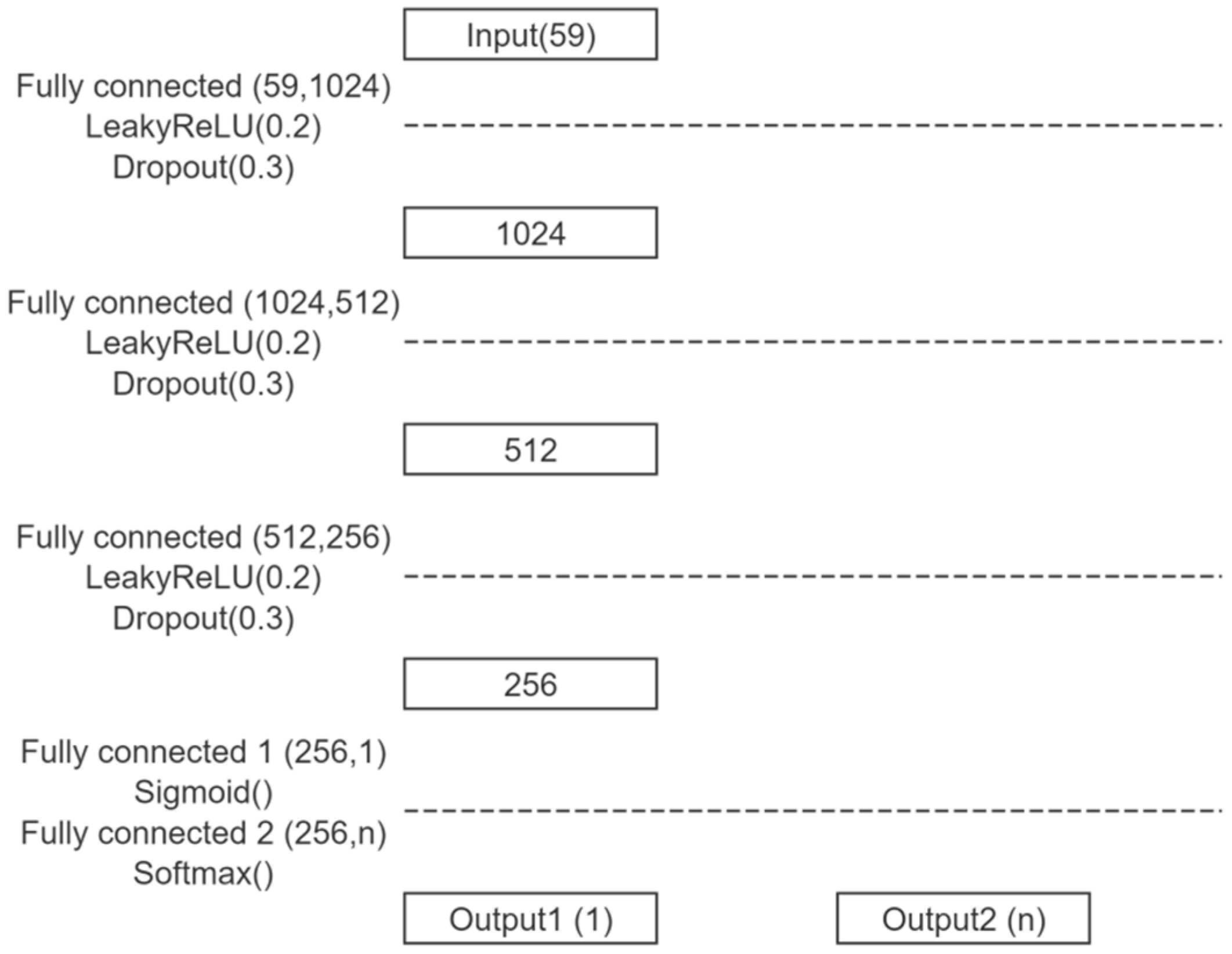
3.2. Discriminator Structure

The discriminator structure of MTC-GAN is shown in Figure 2. Each fully connected layer is equipped with a LeakyReLU activation function and a Dropout layer. This design aims to improve the model’s generalization ability and prevent overfitting. Unlike the discriminator of the original CGAN, the discriminator of this model does not connect the labeled data at the input. This design enables the trained MTC-GAN discriminator to be directly applied to classification tasks. Therefore, the potential influence of labeled data on the structure of the discriminator is avoided during pre-training. In the output part of the discriminator, there is not only a true/false output for authenticity judgment but also an additional output for category prediction. This dual function of combining authenticity assessment and category prediction allows the generator to achieve a more controlled generation process. This not only improves the quality of the generated images but also significantly enhances the usefulness of the model and the accuracy of the classification.

3.3. Model Training and Loss Function

The generator is responsible for generating images from random noise and category labels. The discriminator is required to determine the authenticity of the image and classify the categories of the image. Two main loss functions are used in the training process. They are the Binary Cross-Entropy Loss for judging the authenticity of the image and the Cross Entropy Loss for image classification. The adversarial loss of the discriminator for real samples and generated samples is
L D a d v = y log D x + 1 y log 1 D x
where D is the discriminator, which is used to determine whether the input sample is real or generated; x is real sample; and y is the label of the sample, 1 when the sample is real and 0 for generated samples.
The classification loss of the discriminator for real samples is
L D c l s = C = 1 C t c log D c l s x c
where tc is the label of the category to which the sample belongs; Dcls is the classifier part of the discriminator that classifies the samples; and xc represents real samples belonging to category c.
The adversarial loss of the generator for the generated samples is
L G a d v = log D G z
where z is the noise vector of the input generator; G is the generator for generating fake samples.
The classification loss of the generator for the generated samples is
L G c l s = C = 1 C t c log D c l s G z c
The loss function of the discriminator D is
L D = L D a d v + L D c l s
The loss function of the generator G is
L G = L G a d v + L G c l s
After obtaining the loss function for the discriminator and generator, the Adam optimizer is used to optimize the loss function.

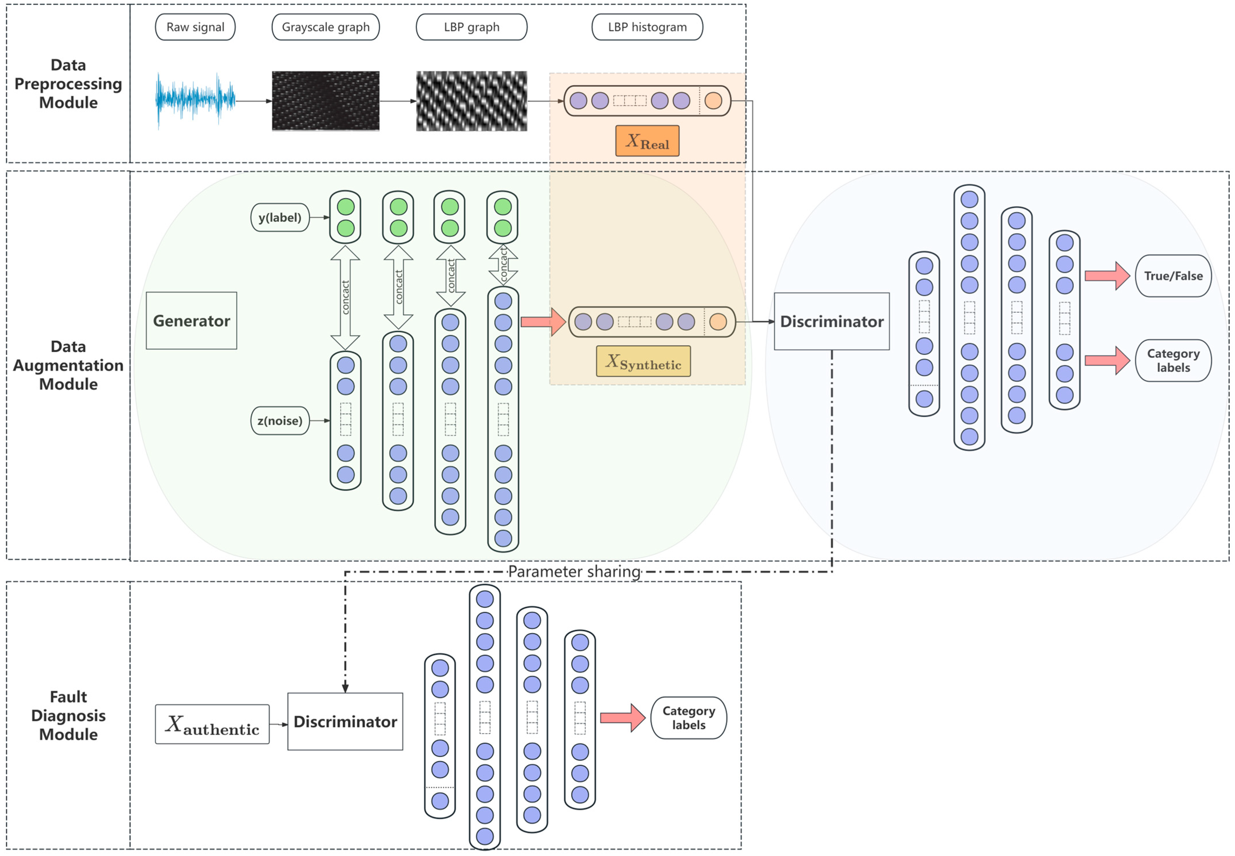
3.4. Modelling Structure

The training mechanism of MTC-GAN is significantly different from traditional GANs. Traditional GANs usually combine generated high-quality samples with real samples for additional classifier training after the model training is completed, as a way to achieve data enhancement and improve model performance. However, MTC-GAN adopts a different strategy. Its discriminators are directly applied to the classification task after training is completed. It does not admit any additional generated samples outside the training process. Therefore, MTC-GAN requires data augmentation during the training process. In this process, additional generated samples are internally and dynamically input into the training. This dynamic input strategy adjusts the timing and quantity of inputs based on the real-time distance between samples generated by the model’s generator and the real samples. This allows the model to continuously adapt and optimize during training. The input of high-quality samples begins after the model is able to generate them consistently. MTC-GAN ensures that the generated samples used can effectively support model training. This significantly improves overall classification performance. The implementation of this training strategy not only enhances the model’s adaptability to complex data environments but also introduces new challenges, placing higher demands on the optimization of the training strategy and model performance.
The general framework of the methodology proposed in this paper is shown in Figure 3, and the main steps are as follows:
Step 1: Acquire acceleration vibration signals of bearings from different categories and correct the signals to eliminate negative values.
Step 2: Design the length and size of individual samples based on physical guidelines and convert them into 2D grayscale maps.
Step 3: Feature extraction of grayscale images using the Local Binary Pattern operator to capture small variations in the signal and texture features. A fault feature signature with high recognition capability is constructed.
Step 4: Use the obtained fault feature signature to train the MTC-GAN model.
Step 5: Extract the discriminator part from the trained MTC-GAN model and apply it to the fault diagnosis task.

4. Experimental Validation
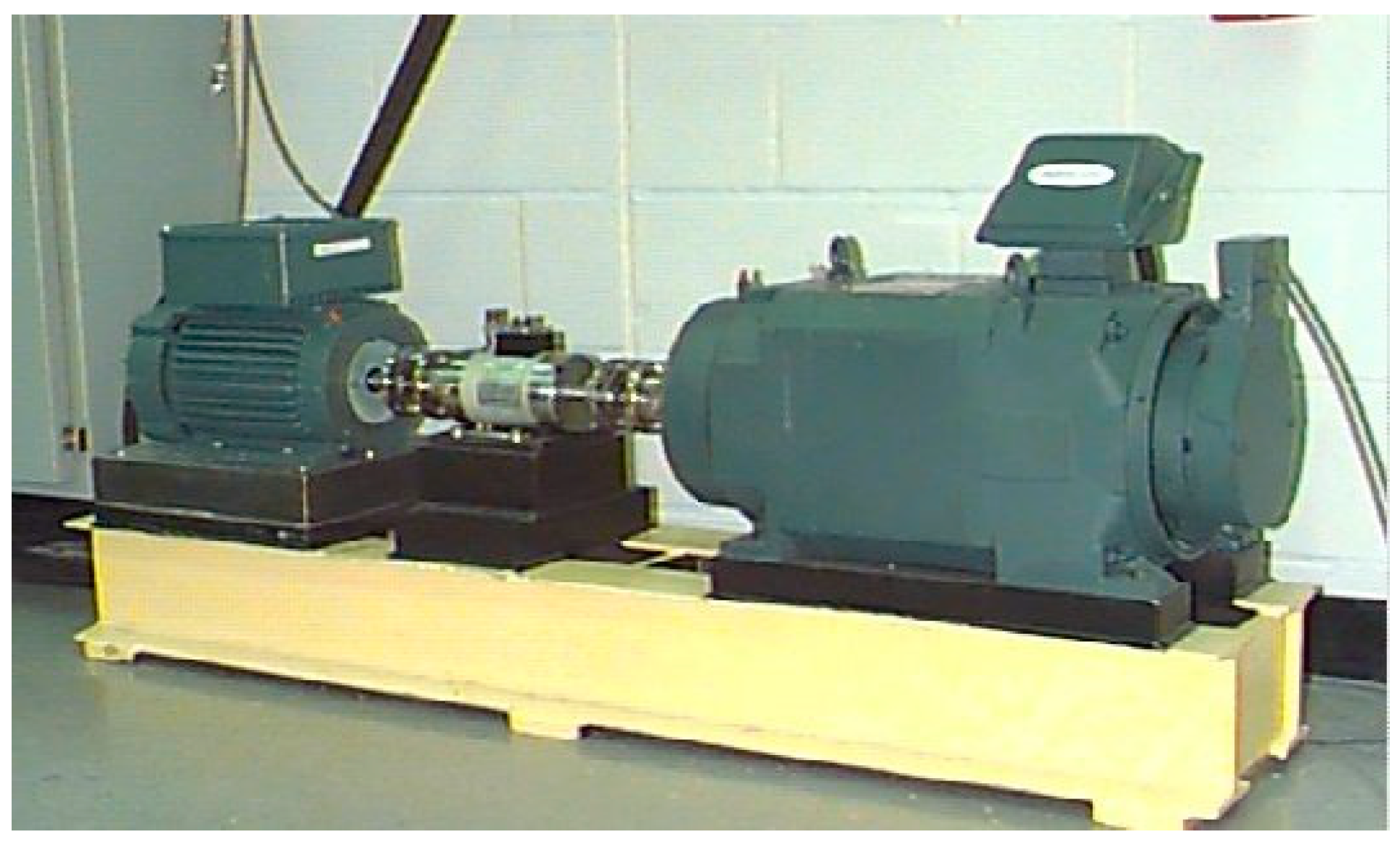
The programming language used in this study is Python 3.9, and the deep learning framework is PyTorch 2.0. The experiments were conducted on a computer equipped with an 11th Gen Intel(R) Core(TM) i7-11800H @ 2.30 GHz processor and 16 GB RAM, running a 64-bit Windows operating system. To accelerate the model training process, an additional GPU with 6 GB memory (RTX 3060) was utilized.

4.1. Data Sets

The experimental data were obtained from the CWRU bearing dataset at the Engineering Centre of Case Western Reserve University (USA). The experimental setup is shown in Figure 4 and includes the drive motor, torque sensor, dynamometer, and bearing unit. To simulate different degrees of bearing failure states, single-point damages were created on the inner ring, outer ring, and rolling elements of the bearings using EDM technology. The damage diameters were 0.007 inch, 0.014 inch, and 0.021 inch, respectively. The data acquisition system consisted of accelerometers mounted on the fan end of the motor and on the drive end bearing housing. Experiments were conducted at a variety of speeds and load conditions, including 1797 rpm, 1772 rpm, 1750 rpm, and 1730 rpm. Loads ranged from 0 to 3 hp. This setup allows for the full simulation of a variety of operating environments.
This study focuses on the vibration acceleration signals of the drive end bearing under different operating conditions at a sampling frequency of 12 kHz. The specifications of the drive end bearings are detailed in Table 1.
The test bearings were set up with a single point of damage on the inner ring, outer ring, and rolling elements. The damage to the outer ring of the bearing was set at three different locations: 3 o’clock, 6 o’clock, and 12 o’clock. To maintain consistency in the analysis and simplify data processing, this paper classifies the damage at these three locations as outer ring failure. The categorized states in this study include four types: normal state, inner ring failure, outer ring failure, and rolling body failure. See Table 2 for details.

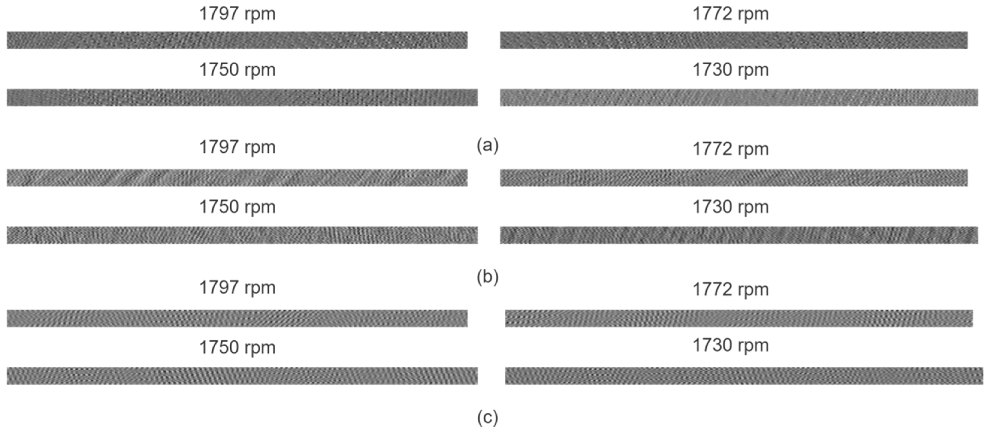
4.2. Image Construction

Before converting the vibration signals to grayscale, it is necessary to select the appropriate image size. This not only ensures the accuracy of the image details but also produces a more uniform and robust texture. Proper image construction will maximize the efficiency of feature extraction. Taking the vibration data at 1797 rpm as an example, firstly, the length of the sample is designed. Then, the theoretical FCFs for the three fault types are calculated. The calculation results are detailed in Table 3. According to Equation (5), we set the sampling factor α to 2 to ensure the integrity of the signal and that the frequency resolution meets the experimental requirements, and the lower limit of the input length is obtained as 224. Finally, according to Equation (6), the new sample length is set as 5333.
After determining the length of the sample, the size of the sample is designed. The width of the sample was determined by the number of measurement points acquired in one axis rotation cycle. The width was determined to be 402 according to Equation (9), and the height was determined to be 14 according to Equation (10). The LBP operator adapts to 3 × 3-pixel blocks. Therefore, the width and height of the samples also need to be in multiples of 3. To prevent the loss of information due to an insufficient sample size, the height was increased to 15. The final sample size was 402 × 15. This ensured that each vibration image contained an integer number of 3 × 3-pixel blocks and eliminated any overlap or loss of vibration data during segmentation and superimposition. No information in the original data was altered or omitted during the image construction process. Using the same methodology, sample sizes were determined for other speeds. The sample size for 1772 rpm was 408 × 15. The sample size for 1750 rpm was 411 × 15. The sample size for 1730 rpm was 417 × 15. Based on the physical information of the bearing, 2D grayscale images were designed and generated as shown in Figure 5.

4.3. Fault Signature Construction

The LBP operator performs a texture analysis on the grayscale map obtained from the conversion of the vibration signals. The LBP operator compares the difference in grayscale values between each pixel in the image and its surrounding pixels. Binary patterns representing local texture information are generated. These binary patterns are further converted into LBP feature maps, as shown in Figure 6. The LBP feature maps reveal the micro-texture properties in the original vibration signal.
In order to simplify the complexity of the input features and reduce the difficulty of training, we used the uniform mode to compile all the local descriptors into a global LBP histogram. This is used as a feature vector to capture the texture distribution across the image. These feature vectors act as unique fault signatures and provide inputs to the subsequent deep learning models. This helps to classify and identify different fault patterns. Uniform patterns are considered more representative and discriminative in texture analysis. By focusing on these uniform patterns, the generated global histogram not only emphasizes the micro-texture structures of the image but also maintains the relative stability of these structures across different rotational speeds. This enables the model to more effectively identify specific texture patterns associated with faults, thereby significantly improving the accuracy and efficiency of fault diagnosis.

4.4. Model Testing

The experimental data were derived from vibration acceleration signals at four rotational speeds: 1797 rpm, 1772 rpm, 1750 rpm, and 1730 rpm. Separate datasets were created at each rotational speed, and the shaft rotational speeds in each dataset were assumed to be constant to exclude random fluctuations in the measurements. Details of the specific datasets can be found in Table 4.
In order to validate the initial accuracy of the model under small sample sizes and variable operating conditions, we set the number of samples for all fault types in the training set for different speed conditions to 1, while the number of normal class samples was set to 10. This setup simulates the scenario of small sample imbalance in practical applications. The initial training was conducted using the discriminator of MTC-GAN to assess the model’s ability to adapt to different operating conditions without increasing the data. The detailed hyperparameters for the MTC-GAN model are shown in Table 5.
The preliminary fault diagnosis results of the bearing under a single working condition are shown in Table 6. To ensure the reliability and accuracy of the experiments, all experiments were repeated 20 times, and the average result was calculated after removing the best and worst results. The experimental results show that the model has achieved good accuracy through the preliminary data preprocessing method. The LBP operator is able to extract information about different types of vibration signals of the bearing. These data will be used as the benchmark before subsequent data enhancement.
After confirming the initial accuracy of the discriminator under small sample imbalanced data conditions, additional training samples were generated using the generator of the MTC-GAN for data augmentation. The trained discriminators were extracted and directly applied to the test set for fault classification. Unlike traditional GANs, MTC-GAN does not combine the generated high-quality samples with real samples for additional classifier training after training is complete. Instead, it internally and dynamically inputs additional generated samples during the training process. As an example, the classification accuracy curve for bearing under the 1797 rpm operating condition is shown in Figure 7. The figure shows the number of samples generated by MTC-GAN in each training round after starting to generate extra generated samples and the specific impact of these samples on the accuracy of the final test set.
As can be seen in Figure 7, after the MTC-GAN model is initially trained and reaches a steady state, the generator gradually acquires more data features. When the quality score of the data generated by the model reaches the agreed scoring threshold (MSE < 0.02, SSIM > 0.90), the model starts to generate high-quality additional samples. The introduction of additional samples begins after the model has steadily generated high-quality samples. This not only ensures the quality and diversity of the training data but also optimizes the model’s adaptability and stability in complex data environments.
As the number of samples added in each round increases, the accuracy of the model on the test set shows an upward trend. Specifically, when the number of additional samples generated per round is two, the model can achieve an accuracy of approximately 96% within the specified number of training rounds. When this number is increased to four, the accuracy further improves to about 98%. Although these increases are significant, they are not as rapid and stable as when the number of additional samples generated per round is six. With six additional samples per round, the model performs best on the test set, achieving 100% accuracy.
Additionally, to further analyze the performance of the MTC-GAN model during training, Figure 8 shows the loss curves of the generator and discriminator. From the curves, it can be observed that in the early stages of training, the discriminator’s loss drops rapidly while the generator’s loss rises. This indicates that the discriminator is initially able to effectively distinguish between real and generated data, whereas the generator has not yet produced high-quality samples. As the training progresses, the generator’s loss gradually decreases while the discriminator’s loss increases slowly, suggesting that the generator is learning to create more realistic data and gradually deceiving the discriminator. After approximately 300 epochs, the loss values for both the generator and discriminator stabilize, indicating that the adversarial training has reached a relatively balanced state, with further convergence in the loss values. Around 350 epochs, the quality of the data generated by the generator reaches the pre-defined evaluation thresholds, and additional samples are generated. As more training samples are introduced, the generator learns to capture more diverse features and characteristics, reducing the discrepancy with the real data, leading to a rapid convergence of the loss, which then fluctuates within a smaller range. This reflects the fine-tuning process of the generator in producing high-quality samples. At this stage, the discriminator retains a certain level of distinguishing ability, while the generator is able to produce higher-quality samples. Overall, the loss curves indicate that the MTC-GAN model has achieved effective adversarial learning during training, gradually reaching equilibrium, with a significant improvement in the quality of the samples generated by the generator.
However, it is worth noting that as the number of additional samples continues to increase, the stability of the model begins to decline, showing noticeable fluctuations. This phenomenon may be attributed to the possibility that an excessive number of generated samples leads the generator to overfit the training data, resulting in instability on the test set. While the increase in additional samples enhances the model’s learning ability to some extent, it also increases the difficulty of learning complex features. Therefore, it is crucial to precisely control the number of additional samples generated in each round, ensuring the quality and diversity of the generated samples while preventing the generator from overfitting, in order to maintain the model’s stability and robustness.
In this experiment, the number of additional samples for each input round was selected to be six. A comparison of the final accuracy obtained under different rotational speed conditions with the initial accuracy is shown in Figure 9. This indicates that the dynamic input strategy enables the MTC-GAN model to demonstrate excellent classification ability in different datasets. The dynamic input strategy can significantly improve the performance of the model. This strategy provides an effective method for GAN model training. It ensures the quality of generated samples while enabling the model to achieve the expected results faster within the specified number of training rounds and optimizes the model’s performance in diverse data environments.
Further, we will focus on analyzing the performance of the model under small sample imbalanced data and varying working conditions. To verify the robustness of the proposed method, four test scenarios are designed. In the first scenario, dataset 1 of 1797 rpm is used to train the classifier, and datasets 2, 3, and 4 of 1772 rpm, 1750 rpm, and 1730 rpm are used as the test sets. In the second scenario, dataset 2 of 1772 rpm serves as the training set, and the remaining datasets serve as the test sets. Similarly, dataset 3 and dataset 4 serve as the training sets, and the rest of the datasets serve as the test sets in the third and fourth scenarios, respectively. This approach involves training the classifier on one speed dataset and testing it on three datasets with different speeds. In this way, the model’s ability to adapt to speed variations is systematically evaluated.
The preliminary diagnostic performance of the model under the above variable operating conditions is detailed in Table 7. This clearly indicates that the proposed method is effective for diagnosing bearing faults and is unaffected by variations in the rotational speed, whether random or planned. As mentioned earlier, this is due to the uniformity of the texture in the vibration images, which were constructed after determining their optimal size.
The comparison of the final accuracy obtained under variable working conditions with the initial accuracy is shown in Figure 10. To analyze the classification performance of the model under different working conditions in more detail, the confusion matrix of the classification results under different scenarios is shown in Figure 11. It can be seen that the classification accuracy of the model for different RPM conditions is maintained at a high level in all four test scenarios. This further proves that the MTC-GAN model can effectively distinguish between different types of faults under variable operating conditions. The MTC-GAN model shows strong robustness and adaptability under these conditions.

4.5. Comparative Experiments

To verify the effectiveness of the proposed method, we conducted two types of experiments: single-condition comparison and varying-condition comparison. In the single-condition experiment, the Support Vector Machine (SVM), Convolutional Neural Network (CNN), and Long Short-Term Memory (LSTM) were selected as comparative models; in the varying-condition experiment, the Deep Transfer Learning (DTL) and Domain Adaptation Network (DAN) models were added. To ensure the fairness of the experiments, all models were trained and tested using the same batch and quantity of vibration signal data points. Before being fed into the models, the data were normalized and presented either as one-dimensional vibration signals or two-dimensional grayscale images, ensuring consistency in the processing across models. The experiments mainly evaluated each model’s average classification accuracy, training time, and testing time.

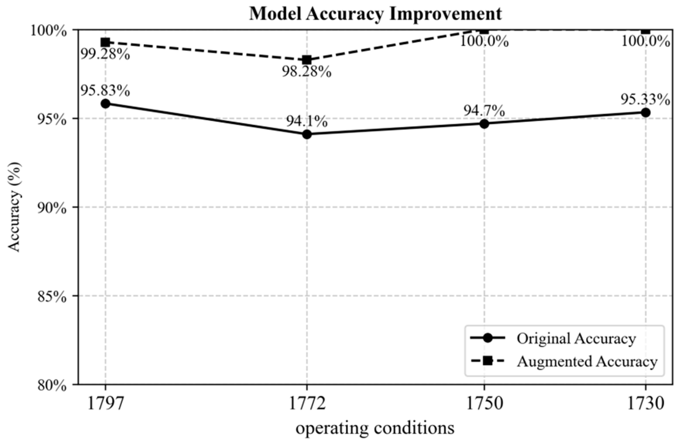
4.5.1. Single-Condition Comparison Experiment

The results of the single-condition comparison experiment are detailed in Table 8. The results show that although SVM has certain advantages in training and testing time, its classification accuracy is much lower than that of the other deep learning models, indicating its limitations in extracting complex signal features. In contrast, CNN and LSTM demonstrate certain advantages in feature extraction and sequence modeling, but they are limited by the small sample size, preventing them from fully learning the data features, which leads to relatively lower classification accuracy. Additionally, their complex network structures result in increased computational overhead. Our proposed method, however, excels in both classification accuracy and computational efficiency. This can be attributed to two key factors: first, the LBP feature extraction method not only effectively captures critical texture features in the vibration signals but also reduces computational complexity by using uniform patterns, significantly accelerating the feature extraction process. Moreover, the lightweight design of MTC-GAN and its inherent data augmentation capability enable the method to achieve a high classification accuracy of 99.28% while also significantly reducing training and testing times to 182 s and 35 s, respectively.

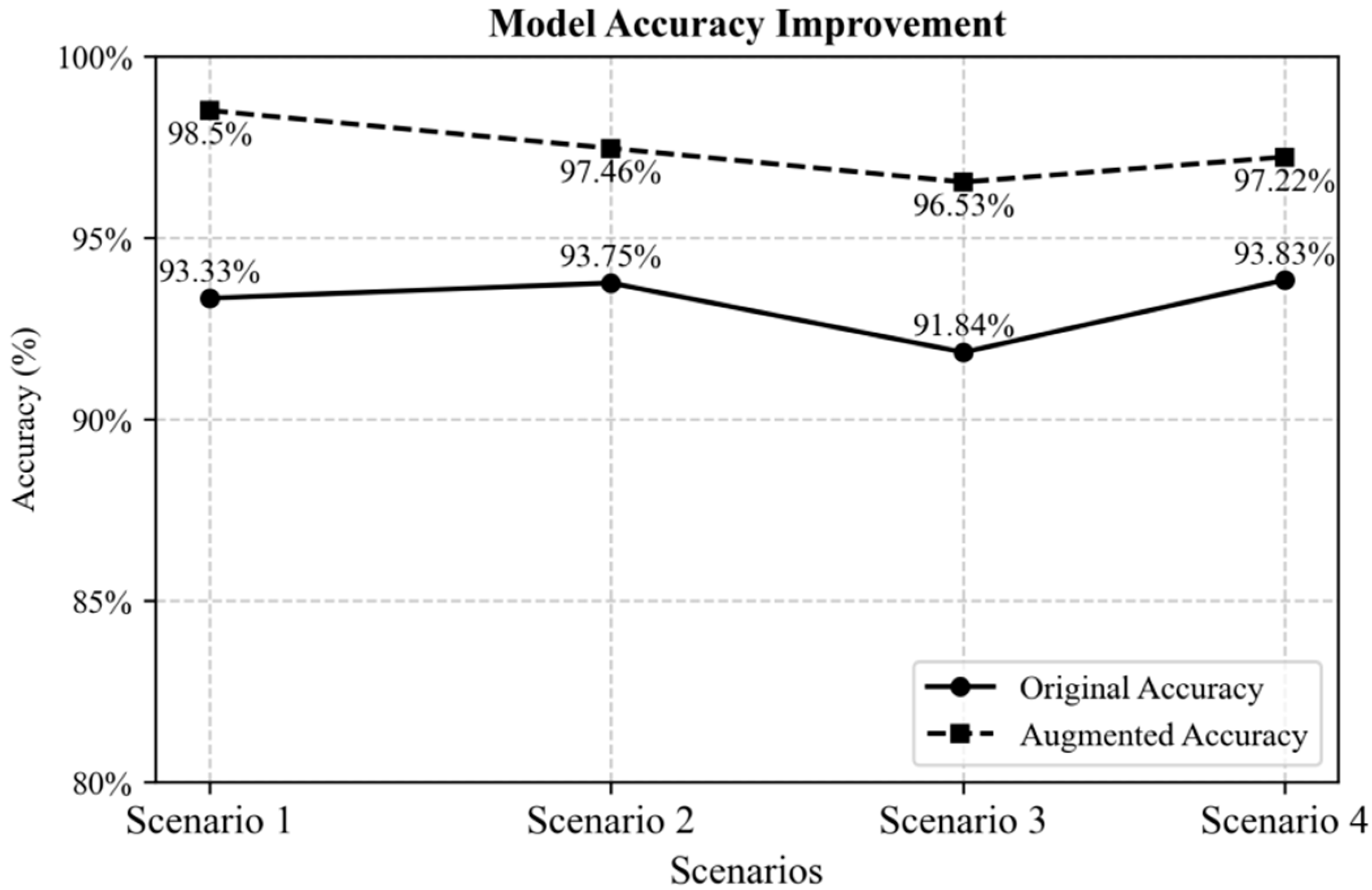
4.5.2. Varying-Condition Comparison Experiment

In the varying-condition experiment, we used Scenario 1 from the previous sections, where the dataset with a speed of 1797 rpm was used as the training set, and datasets with other speeds (1772 rpm, 1750 rpm, and 1730 rpm) were used as the testing sets. On the basis of the single-condition comparison experiment, we added the DTL and DAN models to evaluate the classification accuracy, training time, and testing time of each model under varying working conditions. Each experiment was also repeated 20 times, and the average result was taken as the final result, as shown in Table 9.
The experimental results show that under varying conditions, the classification performances of SVM, CNN, and LSTM drop significantly, indicating that these models struggle to effectively capture the signal feature changes caused by the varying conditions. In contrast, the DTL and DAN models, through transfer learning and domain adaptation techniques, improved the adaptability of the models to different working conditions, with classification accuracies of 91.56% and 93.43%, respectively, demonstrating good robustness. However, these methods performed suboptimally in small-sample environments, particularly when faced with the dual challenges of condition variation and insufficient sample size. In comparison, our proposed MTC-GAN model maintained excellent performance under both small-sample and varying-condition scenarios, achieving a classification accuracy of 98.50% while keeping training and testing times relatively short. These results fully demonstrate the high efficiency and broad applicability of the proposed method in real-world applications. This confirms that the method is not only capable of maintaining high accuracy but also offers exceptional computational efficiency, making it well-suited for practical fault diagnosis tasks.

5. Conclusions

To overcome the dual challenges of small sample data and variable operating conditions, this paper proposes a novel bearing fault diagnosis method that combines physics-guided two-dimensional signal analysis with the MTC-GAN model. First, the physical characteristics of vibration acceleration signals are analyzed to generate two-dimensional vibration signal images. Then, the Local Binary Pattern (LBP) operator is employed to extract the micro-texture features of the images, thereby constructing highly discriminative fault feature signatures. Finally, the MTC-GAN model is utilized for data augmentation, generating high-quality synthetic samples to enhance the generalization capability under small sample conditions, and the model’s discriminator is used to perform fault classification tasks. This method significantly improves the model’s adaptability and classification accuracy under small sample sizes and varying operating conditions.
The experimental results demonstrate that the proposed method maintains excellent classification accuracy and robustness, even under limited training data, in both single and variable operating conditions. Compared to traditional fault diagnosis methods, the proposed approach exhibits superior diagnostic accuracy and efficiency. Future research could focus on further exploring bearing fault diagnosis under complex scenarios involving small samples and variable operating conditions, by developing more advanced feature extraction techniques and optimizing model architectures to enhance fault detection accuracy and model adaptability in diverse working conditions.

Author Contributions

Conceptualization, X.G. and J.L.; methodology, X.G. and J.L.; software, X.G. and Y.W.; validation, X.G. and J.L.; formal analysis, J.L.; investigation, J.L.; resources, J.L.; data curation, Y.W. and J.L.; writing—original draft preparation, X.G.; writing—review and editing, Y.W. All authors have read and agreed to the published version of the manuscript.

Funding

This work was supported by the Scientific Research Fund of Department of Education of Liaoning Province, China (LJKZZ20220037).

Institutional Review Board Statement

Not applicable.

Informed Consent Statement

Not applicable.

Data Availability Statement

The data presented in this study are available on request from the corresponding author. The raw/processed data needed to reproduce these findings cannot be shared publicly at this time, as they are also part of ongoing study.

Conflicts of Interest

The authors declare no conflicts of interest.

References

  1. Song, Q.; Jiang, X.; Du, G.; Liu, J.; Zhu, Z. Smart Multichannel Mode Extraction for Enhanced Bearing Fault Diagnosis. Mech. Syst. Signal Process. 2023, 189, 110107. [Google Scholar] [CrossRef]
  2. Chaleshtori, A.E.; Aghaie, A. A Novel Bearing Fault Diagnosis Approach Using the Gaussian Mixture Model and the Weighted Principal Component Analysis. Reliab. Eng. Syst. Saf. 2024, 242, 109720. [Google Scholar] [CrossRef]
  3. Zhang, B.; Li, F.; Ma, N.; Ji, W.; Ng, S.-K. Open Set Bearing Fault Diagnosis with Domain Adaptive Adversarial Network under Varying Conditions. Actuators 2024, 13, 121. [Google Scholar] [CrossRef]
  4. Wang, J.; Ahmed, H.; Chen, X.; Yan, R.; Nandi, A.K. Improved Adversarial Transfer Network for Bearing Fault Diagnosis under Variable Working Conditions. Appl. Sci. 2024, 14, 2253. [Google Scholar] [CrossRef]
  5. Lourari, A.W.; Soualhi, A.; Benkedjouh, T. Advancing Bearing Fault Diagnosis under Variable Working Conditions: A CEEMDAN-SBS Approach with Vibro-Electric Signal Integration. Int. J. Adv. Manuf. Technol. 2024, 132, 2753–2772. [Google Scholar] [CrossRef]
  6. Chen, X.; Wang, Z.; Zhang, Z.; Jia, L.; Qin, Y. A Semi-Supervised Approach to Bearing Fault Diagnosis under Variable Conditions towards Imbalanced Unlabeled Data. Sensors 2018, 18, 2097. [Google Scholar] [CrossRef]
  7. Jin, Z.; Sun, Y. Research on Bearing Variable Condition Fault Diagnosis Based on RDADNN. J. Fail. Anal. Prev. 2023, 23, 1663–1674. [Google Scholar] [CrossRef]
  8. Peng, C.; Zhang, S.; Li, C. A Rolling Bearing Fault Diagnosis Based on Conditional Depth Convolution Countermeasure Generation Networks under Small Samples. Sensors 2022, 22, 5658. [Google Scholar] [CrossRef] [PubMed]
  9. Pan, B.; Wang, W.; Wen, J.; Li, Y. Semi-Supervised Adversarial Transfer Networks for Cross-Domain Intelligent Fault Diagnosis of Rolling Bearings. Appl. Sci. 2023, 13, 2626. [Google Scholar] [CrossRef]
  10. Di Maggio, L.G.; Brusa, E.; Delprete, C. Zero-Shot Generative AI for Rotating Machinery Fault Diagnosis: Synthesising Highly Realistic Training Data via Cycle-Consistent Adversarial Networks. Appl. Sci. 2023, 13, 12458. [Google Scholar] [CrossRef]
  11. Ruan, D.; Chen, X.; Gühmann, C.; Yan, J. Improvement of Generative Adversarial Network and Its Application in Bearing Fault Diagnosis: A Review. Lubricants 2023, 11, 74. [Google Scholar] [CrossRef]
  12. Kwon, H. Adversarial Image Perturbations with Distortions Weighted by Color on Deep Neural Networks. Multimed. Tools Appl. 2023, 82, 13779–13795. [Google Scholar] [CrossRef]
  13. Kwon, H.; Kim, S. Dual-Mode Method for Generating Adversarial Examples to Attack Deep Neural Networks. IEEE Access 2023. [Google Scholar] [CrossRef]
  14. Ruan, D.; Wang, J.; Yan, J.; Gühmann, C. CNN Parameter Design Based on Fault Signal Analysis and Its Application in Bearing Fault Diagnosis. Adv. Eng. Inform. 2023, 55, 101877. [Google Scholar] [CrossRef]
  15. Khan, S.A.; Kim, J.-M. Automated Bearing Fault Diagnosis Using 2D Analysis of Vibration Acceleration Signals under Variable Speed Conditions. Shock. Vib. 2016, 8729572. [Google Scholar] [CrossRef]
  16. Goodfellow, I.; Pouget-Abadie, J.; Mirza, M.; Xu, B.; Warde-Farley, D.; Ozair, S.; Courville, A.; Bengio, Y. Generative Adversarial Nets. Adv. Neural Inf. Process. Syst. 2014, 2, 2672–2680. [Google Scholar]
  17. Mirza, M.; Osindero, S. Conditional Generative Adversarial Nets. Comput. Sci. 2014, 2672–2680. [Google Scholar] [CrossRef]
Figure 1. Generator structure diagram.
Applsci 14 08791 g001
Figure 2. Discriminator structure diagram.
Applsci 14 08791 g002
Figure 3. Proposed framework diagram for bearing fault diagnosis under small sample size and variable operating conditions.
Applsci 14 08791 g003
Figure 4. Case Western Reserve University (CWRU) bearing test bench.
Applsci 14 08791 g004
Figure 5. The vibration images for (a) the inner race fault, (b) the ball, and (c) the outer race fault.
Applsci 14 08791 g005
Figure 6. The LBP images for (a) the inner race fault, (b) the ball, and (c) the outer race fault.
Applsci 14 08791 g006
Figure 7. Test set accuracy curves with different numbers of additional generated samples at 1797 rpm.
Applsci 14 08791 g007
Figure 8. The generator loss and discriminator loss curves of the MTC-GAN model.
Applsci 14 08791 g008
Figure 9. Final accuracy vs. initial accuracy at different rotational speeds.
Applsci 14 08791 g009
Figure 10. Final accuracy vs. initial accuracy under variable operating conditions.
Applsci 14 08791 g010
Figure 11. Confusion matrix for classification results: (a) Scenario 1; (b) Scenario 2; (c) Scenario 3; and (d) Scenario 4.
Applsci 14 08791 g011
Table 1. Specifications of bearings.
AttributeValue
ModelJEM SKF 6205-2RS (SKF, Gothenburg, Sweden)
LocationDriver end
Outside diameter2.0472 inches
Inside diameter0.9843 inches
Thickness0.5906 inches
Ball diameter0.3126 inches
Pitch diameter1.537 inches
Table 2. Specifications of fault types.
Fault TypeFault LocationFault Diameter
(Inches)
Fault Depth
(Inches)
Inner raceway fault
(IRF)
Inner raceway0.0070.011
Outer raceway fault
(ORF)
Outer raceway0.0070.011
Ball fault(BF)Ball0.0070.011
NormalNilNilNil
Table 3. Theoretical fault characteristic frequency of CWRU datasets.
FCF (Hz)Order
1st2nd3rd4th5th
f O R 107.36214.72322.08429.44536.80
f I R 162.19324.38486.57648.76810.95
f b a l l 141.17282.34423.51564.68705.85
Table 4. Datasets for the proposed fault diagnosis scheme.
DatasetsFault TypeShaft Speed
(rpm)
Motor Load
(hp)
Number of CyclesNumber of Samples
1Inner raceway17970~30220
Outer raceway17970~30460
Ball17970~30520
Normal17970~60840
2Inner raceway17721~30019
Outer raceway17721~30158
Ball17721~29819
Normal17721~119080
3Inner raceway17502~29619
Outer raceway17502~29558
Ball17502~29419
Normal17502~117779
4Inner raceway17303~29319
Outer raceway17303~29358
Ball17303~29020
Normal17303~161578
Table 5. Hyperparameter settings for the MTC-GAN model.
HyperparameterValue
Generator Learning Rate0.0002
Discriminator Learning Rate0.0002
Batch Size4
Number of Epochs500
Noise Dimension100
Table 6. Initial diagnostic performance of the method under single operating conditions.
Training Datasets
(Number of Training Samples)
Testing Datasets
(Number of Test Samples)
Classification Accuracy (%)Average Classification Accuracy (%)
Ball Fault
(BF)
Inner Race Fault
(IRF)
Outer Race Fault
(ORF)
Normal
Dataset 1797 (15)Dataset 1797 (125)94.7292.7695.84100.0095.83
Dataset 1772 (15)Dataset 1772 (162)92.2891.3394.2398.5694.10
Dataset 1750 (15)Dataset 1750 (160)93.4991.5695.3398.4094.70
Dataset 1730 (15)Dataset 1730 (160)93.7893.2094.3510095.33
Table 7. Initial diagnostic performance of the proposed method in different scenarios.
Training Datasets
(Number of Training Samples)
Testing Datasets
(Number of Test Samples)
Classification Accuracy (%)Average Classification Accuracy (%)
Ball Fault
(BF)
Inner Race Fault
(IRF)
Outer Race Fault
(ORF)
Normal
Dataset 1 (15)Dataset 2, 3, 4 (527)90.1392.2892.8399.4893.33
Dataset 2 (15)Dataset 1, 3, 4 (490)90.8992.4492.0699.6193.75
Dataset 3 (15)Dataset 1, 2, 4 (492)92.8088.9194.2098.5391.84
Dataset 4 (15)Dataset 1, 2, 3 (492)93.3486.5096.2099.2893.83
Table 8. Comparative test results between different models under single-condition conditions.
ModelClassification Accuracy (%)Training Time (s)Testing Time (s)
SVM75.3214427
CNN90.4596262
LSTM92.87108974
Proposed Method99.2818235
Table 9. Comparative test results between different models under varying-condition conditions.
ModelClassification Accuracy (%)Training Time (s)Testing Time (s)
SVM65.83144102
CNN80.47962233
LSTM83.641089278
DTL91.56705254
DAN93.43682194
Proposed Method98.50182131
Disclaimer/Publisher’s Note: The statements, opinions and data contained in all publications are solely those of the individual author(s) and contributor(s) and not of MDPI and/or the editor(s). MDPI and/or the editor(s) disclaim responsibility for any injury to people or property resulting from any ideas, methods, instructions or products referred to in the content.

