M2Former: Multiscale Patch Selection for Fine-Grained Visual Recognition

Abstract

Recently, Vision Transformers (ViTs) have been actively applied to fine-grained visual recognition (FGVR). ViT can effectively model the interdependencies between patch-divided object regions through an inherent self-attention mechanism. In addition, patch selection is used with ViT to remove redundant patch information and highlight the most discriminative object patches. However, existing ViT-based FGVR models are limited to single-scale processing, and their fixed receptive fields hinder representational richness and exacerbate vulnerability to scale variability. Therefore, we propose MultiScale Patch Selection (MSPS) to improve the multiscale capabilities of existing ViT-based models. Specifically, MSPS selects salient patches of different scales at different stages of a MultiScale Vision Transformer (MS-ViT). In addition, we introduce Class Token Transfer (CTT) and MultiScale Cross-Attention (MSCA) to model cross-scale interactions between selected multiscale patches and fully reflect them in model decisions. Compared with previous Single-Scale Patch Selection (SSPS), our proposed MSPS encourages richer object representations based on feature hierarchy and consistently improves performance from small-sized to large-sized objects. As a result, we propose M2Former, which outperforms CNN-/ViT-based models on several widely used FGVR benchmarks.

1. Introduction

Despite recent rapid advances, fine-grained visual recognition (FGVR) is still one of the nontrivial tasks in the computer vision community. Unlike conventional recognition tasks, FGVR aims to predict subordinate categories of a given object, e.g.,  subcategories of birds [1], flowers [2,3], and cars [4,5]. It is a highly challenging task due to inherently subtle inter-class differences caused by similar subordinate categories and large intraclass variations caused by object pose, scale, or deformation.

The most common solution for FGVR is to decompose the target object into multiple local parts [6,7,8,9,10]. Due to subtle differences between fine-grained categories mostly residing in the unique properties of object parts [11], decomposed local parts provide more discriminative clues of the target object. For example, a given bird object can be decomposed into its beak, wing, and head parts. At this time, ‘Glaucous Winged Gull’ and ‘California Gull’ can be distinguished by comparing their corresponding object parts. Early approaches of these part-based methods find discriminative local parts using manual part annotations [6,7,11]. However, curating manual annotations for all possible object parts is labor-intensive and carries the risk of human error [12]. Therefore, the research focus has consequently shifted to a weakly supervised manner [8,9,10,13,14,15]. Researchers use additional tricks such as attention mechanisms [9,14,16] or region proposal networks (RPNs) [13,15,17] to estimate local parts with only category-level labels. However, the part proposal process greatly increases the overall computational cost. Additionally, they tend not to deeply consider the interactions between estimated local parts that are essential for accurate recognition [18].

Recently, Vision Transformers (ViTs) [19] are being actively applied to FGVR [18,20,21,22,23,24,25,26,27]. Relying exclusively on the Transformer [28] architecture, ViTs have shown competitive image classification performance on a large scale. Similar to token sequences in NLP, ViTs embed the input images into fixed-size image patches, and the patches pass through multiple Transformer encoder blocks. Patch-by-patch processing is highly suitable for FGVR because each image patch can be considered as a local part. This means that the cumbersome part proposal is no longer necessary. Additionally, the self-attention mechanism [28] inherent in each encoder block facilitates the modeling of global interactions between patch-divided local parts. ViT-based FGVR methods use patch selection to further boost performance [18,20,21,22]. Because ViTs deal with all patch-divided image regions equally, many irrelevant patches may lead to inaccurate recognition. Similar to part proposals, patch selection selects the most salient patches from a set of generated image patches based on the computed importance ranking, i.e., accumulated attention weights [21,29]. As a result, redundant patch information is filtered out, and only selected salient patches are considered for the final decision.

However, the existing ViT-based FGVR methods suffer from their single-scale limitations. ViTs use fixed-size image patches throughout the entire network, ensuring that the receptive fields remain the same across all layers and preventing ViTs from obtaining multiscale feature representations [30,31,32]. On the other hand, Convolutional Neural Networks (CNNs) are suitable for multiscale feature representations thanks to their staged architecture, where feature resolution decreases as layer depth increases [33,34,35,36,37]. In the early stages, spatial details of an object are encoded on high-resolution feature maps, and as the stages deepen, the receptive field expands with decreasing feature resolution, and higher-order semantic patterns are encoded into low-resolution feature maps. Multiscale features are important for most vision tasks, especially pixel-level dense prediction tasks, e.g., object detection [38,39,40], and segmentation [41,42,43]. In the same context, single-scale processing can cause two failure cases in FGVR, which leads to suboptimal recognition performance. (i) First, it is vulnerable to scale changes in fine-grained objects [32,35,38]. Fixed patch size may be insufficient to capture very subtle features of small-scale objects due to too coarse patches, and conversely, discriminative features may be over-decomposed for large-scale objects due to too finely split patches. (ii) Second, single-scale processing limits representational richness for objects [30,39]. Compared with a CNN that explores rich feature hierarchies from multiscale features, ViT considers only monotonic single-scale features due to its fixed receptive field.

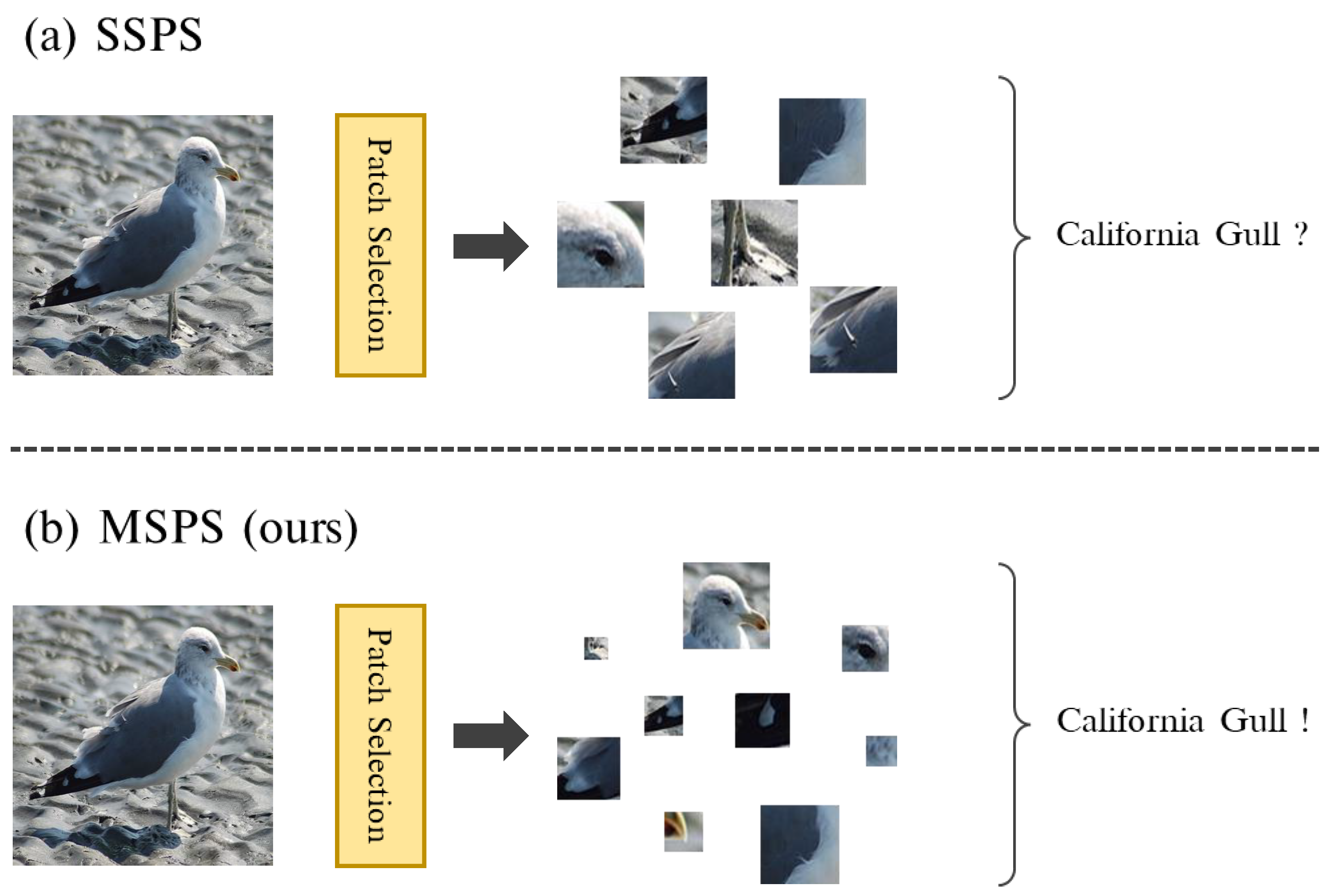
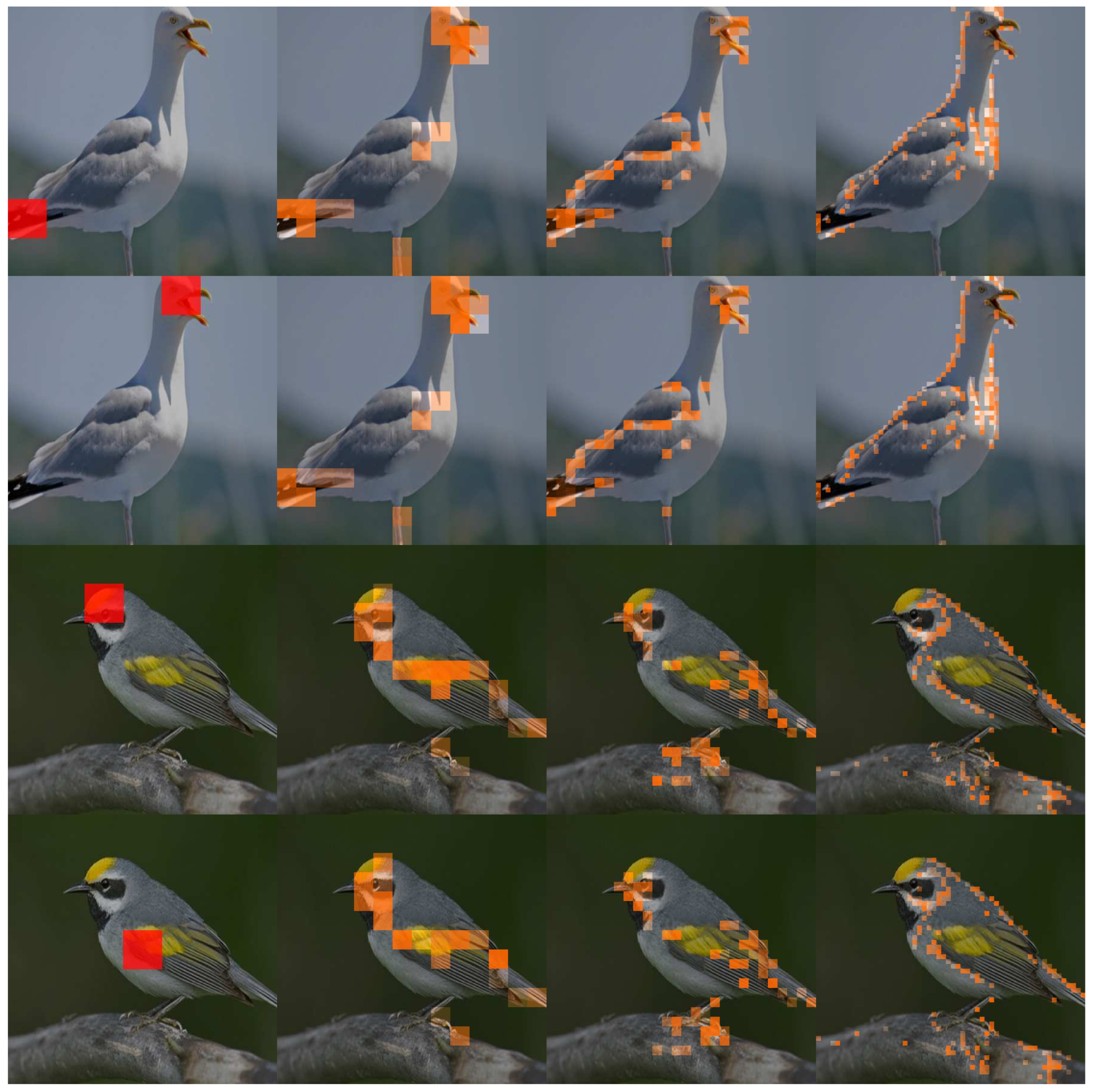
In this paper, we improve existing ViT-based FGVR methods by enhancing multiscale capabilities. One simple solution is to use the recent MultiScale Vision Transformers (MS-ViTs) [30,31,32,44,45,46,47,48,49]. In fact, we can achieve satisfactory results simply by using MS-ViTs. However, we further boost the performance by adapting patch selection to MS-ViTs. Specifically, we propose a MultiScale Patch Selection (MSPS) that extends the previous Single-Scale Patch Selection (SSPS) [18,20,21,22] to multiscale. MSPS selects salient patches of different scales from different stages of the MS-ViT backbone. 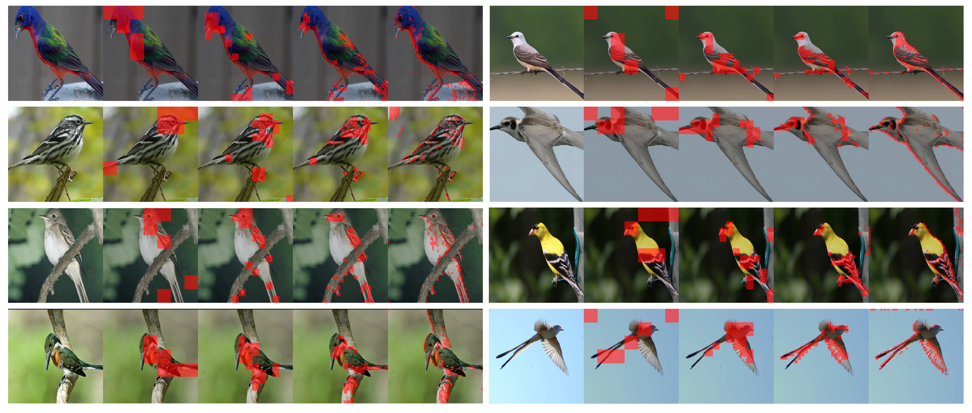As shown in Figure 1, multiscale salient patches selected through MSPS include both large-scale patches that capture object semantics and small-scale patches that capture fine-grained details. Compared with single-scale patches in SSPS, feature hierarchies in multiscale patches provide richer representations of objects, which leads to better recognition performance. In addition, the flexibility of multiscale patches is useful for handling extremely large/small objects through multiple receptive fields.

However, we argue that patch selection alone cannot fully explain the object, and consideration is required for how to model interactions between selected patches and effectively reflect them in the final decision. It is more complicated than considering only single-scale patches. Therefore, we introduce Class Token Transfer (CTT) and MultiScale Cross-Attention (MSCA) to effectively deal with selected multiscale patches. First, CTT aggregates the multiscale patch information by transferring the global CLS token to each stage. Each stage-specific patch information is shared through transferred global CLS tokens, which generate richer network-level representations. In addition, we propose MSCA to model direct interactions between selected multiscale patches. In the MSCA block, cross-scale interactions in both spatial and channel dimensions are computed for selected patches of all stages. Finally, our MultiScale Vision Transformer with MultiScale Patch Selection (M2Former) obtains improved FGVR performance over other ViT-based SSPS models, as well as CNN-based models.

Our main contributions can be summarized as follows:

• We propose MultiScale Patch Selection (MSPS) that further boosts the multiscale capabilities of MS-ViTs. Compared with Single-Scale Patch Selection (SSPS), MSPS generates richer representations of fine-grained objects with feature hierarchies, and obtains flexibility for scale changes with multiple receptive fields.
• We propose Class Token Transfer (CTT) that effectively shares the selected multiscale patch information. Stage-specific patch information is shared through transferred global CLS tokens to generate enhanced network-level representations.
• We design a MultiScale Cross-Attention (MSCA) block to capture the direct interactions of selected multiscale patches. In the MSCA block, the spatial-/channel-wise cross-scale interdependencies can be captured.
• Extensive experimental results on widely used FGVR benchmarks show the superiority of our M2Former over conventional methods. In short, our M2Former achieves an accuracy of 92.4% on Caltech-UCSD Birds (CUB) [1] and 91.1% on NABirds [50].

2. Related Work

2.1. Part-Based FGVR

A number of methods have been proposed to classify subordinate object categories [6,7,11,12,13,14,15,51,52,53,54,55,56,57]. Among them, part-based methods decompose target objects into multiple local parts to capture more discriminative features [6,7,11,13,14,51]. Encoded local representations can be used either in conjunction with image-level representations or by themselves for recognition. This entails the use of a detection branch to generate discriminative part proposals from the input image either before or in parallel with the classification layer. Early works leverage manual part annotations for a fully supervised train of detection branches [6,7,11]. However, curating large-scale part annotations is labor-intensive and highly susceptible to human error. Thus, recent part-based methods localize informative regions in a weakly supervised way using only category-level labels [9,13,14,15,16,17,51,58,59,60,61]. TASN [10] introduces trilinear attention sampling to generate detail-preserved views based on feature channels. P2P-Net [8] and DF-GMM [62] use a Feature Pyramid Network (FPN) [35] to generate local part proposals from convolutional feature maps. RA-CNN [51] iteratively zooms in on local discriminative regions and reinforces multiscale feature learning with interscale ranking loss. InSP [63] extracts potential part regions from the attention maps of two different images and applies content swapping to learn fine-grained local structures. These part-based methods are good at locating discriminative parts, but they are ambiguous at capturing interactions between estimated local parts. Additionally, explicitly generating region proposals incurs a large computational burden, and performance can degrade significantly if the generated proposals are inaccurate. Thus, we focus on ViT-based FGVR methods that can avoid cumbersome region proposals.

2.2. ViT-Based FGVR

Transformer [28] was originally introduced in the natural language processing (NLP) community and has recently shown great potential in the field of computer vision. Specifically, Vision Transformers (ViTs) [19] have recorded remarkable performance in image classification on large-scale datasets relying entirely on a pure Transformer encoder architecture. ViTs split images into nonoverlapping patches and then apply multiple Transformer encoder blocks, consisting of multihead self-attention modules and feed-forward networks. Recently, ViTs have been actively applied to FGVR [18,20,21,22,23,24,25,26,27]. ViTs are highly suitable for FGVR in that (i) patch-by-patch processing can effectively replace part proposal generation, and (ii) it is easy to model global interactions between patch-divided local parts through the inherent self-attention mechanism. In most cases, patch selection, which selects discriminative patches from an initial patch sequence, is used with ViT-based models. TransFG [18] selects the most discriminative patches based on the attention score at the last encoder block to consider only the important image regions. Similarly, DCAL [20] conducts patch selection based on attention scores to highlight the interaction of high-response image regions. FFVT [22] extends this selection process to all layers of ViT to utilize layer-wise patch information. RAMS-Trans [21] enhances local representations by recurrently zooming in on salient object regions obtained by patch selection. For the same purpose, we use patch selection to strengthen the decisiveness of the network. However, we extend the existing patch selection from single-scale to multiscale to improve representational richness and obtain flexibility for scale changes.

2.3. Multiscale Processing

Multiscale features are important for most vision tasks, e.g., object detection [34,35,38,39,40], semantic segmentation [41,42,43], edge detection [64,65], and image classification [33,66,67], because visual patterns occur at multiscales in natural scenes. CNNs naturally learn coarse-to-fine multiscale features through a stack of convolutional operators [68,69], so most research has been proposed to enhance the multiscale capabilities of CNNs [33,34,35,36,37]. FPN [35] introduces a feature pyramid to extract features with different scales from a single image and fuses them in a top-down way to generate a semantically strong multiscale feature representation. SPPNet [33] proposes spatial pyramid pooling to improve backbone networks to model multiscale features of arbitrary size. Faster R-CNN [38] proposes region proposal networks that generate object bounding boxes of different scales. FCN [36] proposes a fully convolutional architecture that generates dense prediction maps for semantic segmentation from hierarchical representations of CNNs.

On the other hand, ViTs suffer from being unsuitable to handle multiscale features due to fixed-scale image patches. After the initial patch embedding layer, ViTs maintain image patches of the same size, and these single-scale feature maps are not suitable for many vision tasks, especially those requiring pixel-level dense prediction. To alleviate this issue, model architectures that adapt multiscale feature hierarchies to ViTs have recently been proposed. CvT [44] adapts convolutional operations to patch embedding layers and attention projection layers to enable feature hierarchies with improved efficiency. MViT [30] introduces attention pooling that controls feature resolution by adjusting the pooling stride of queries to implement multiscale feature hierarchies. PVT [31] proposes a progressive shrinking strategy that conducts patch embedding with different patch sizes at the beginning of each stage. SwinT [32] generates multiresolution feature maps by merging adjacent local patches using a patch merging layer. We also focus on feature hierarchies of fine-grained objects using MS-ViTs. However, we propose additional methods to further boost the multiscale capability, i.e., MSPS, CTT, and MSCA.

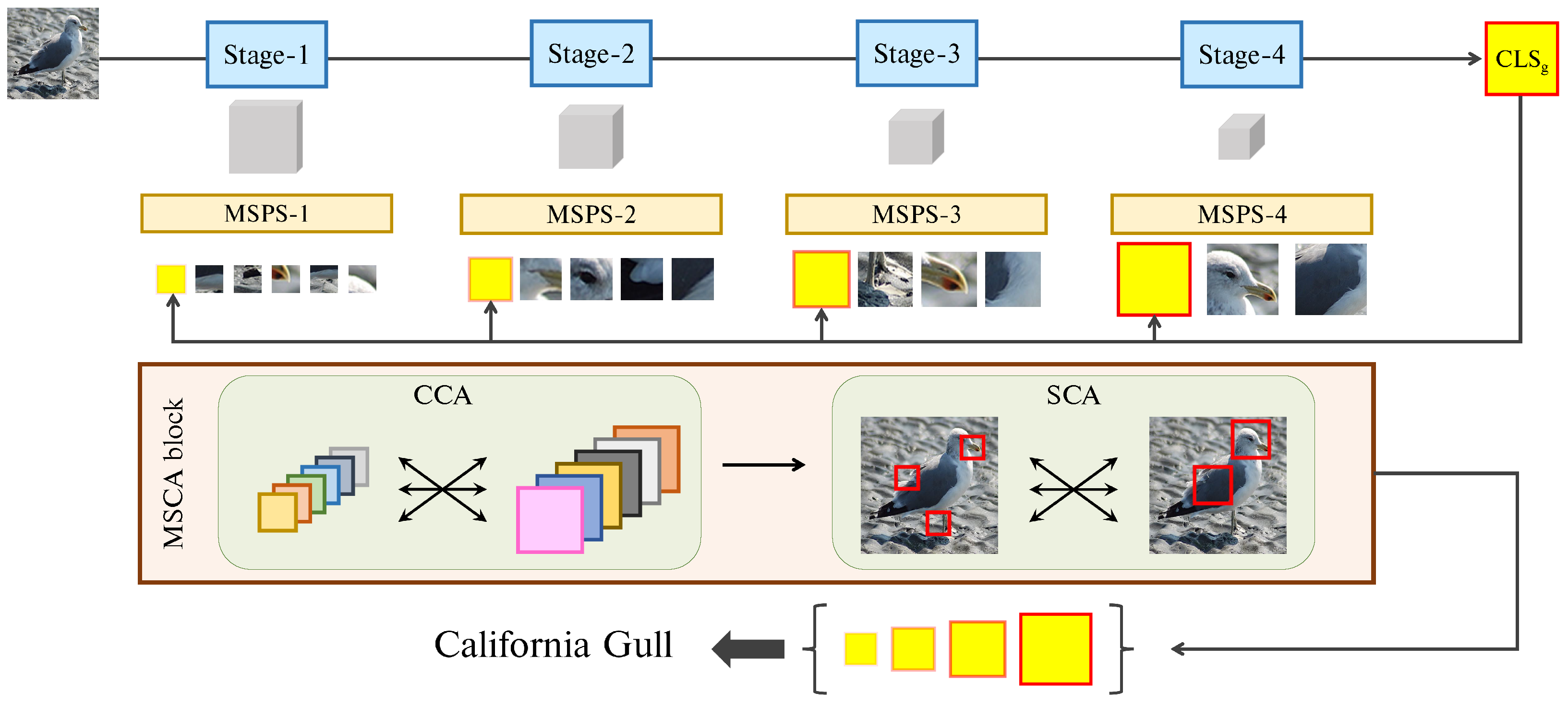
3. Our Method

The overall framework of our method is presented in Figure 2. First, we use MultiScale Vision Transformers (MS-ViTs) as our backbone network (Section 3.1). After that, MultiScale Patch Selection (MSPS) is equipped on different stages of MS-ViT to extract multiscale salient patches (Section 3.2). Class Token Transfer (CTT) aggregates multiscale patch information by transferring the global CLS token to each stage. MultiScale Cross-Attention (MSCA) blocks are used to model spatial-/channel-wise interactions of selected multiscale patches (Section 3.4). Finally, we use additional training strategies for better optimization (Section 3.5). More details are described as follows.

3.1. Multiscale Vision Transformer

To enhance the multiscale capability, we use MS-ViT as our backbone network, specifically the recent Multiscale Vision Transformer (MViT) [30,45]. MViT constructs a four-stage pyramid structure for low-level to high-level visual modeling instead of single-scale processing. To produce a hierarchical representation, MViT introduces Pooling Attention (PA), which pools query tensors to control the downsampling factor. We refer the interested reader to the original work [30,45] for details.

Let $X_0\in {\mathbb{R}}^{h_0\times w_0\times c_0}$ denote the input image, where $h_0$, $w_0$, and $c_0$ refer to the height, width, and the number of channels, respectively. $X_0$ first goes through a patch embedding layer to produce initial feature maps with a patch size of $4\times 4$. As the stage deepens, the resolution of the feature maps decreases and the channel dimension increases proportionally. As a result, at each stage $i\in \{1,2,3,4\}$, we can extract the feature maps $X_i\in \{X_1,X_2,X_3,X_4\}$ with resolutions $h_i\times w_i\in \{{\displaystyle \frac{h_0}{4}}\times {\displaystyle \frac{w_0}{4}},{\displaystyle \frac{h_0}{8}}\times {\displaystyle \frac{w_0}{8}},{\displaystyle \frac{h_0}{16}}\times {\displaystyle \frac{w_0}{16}},{\displaystyle \frac{h_0}{32}}\times {\displaystyle \frac{w_0}{32}}\}$ and channel dimensions $c_i\in \{96,192,384,768\}$. We can also flatten $X_i$ into 1D patch sequence as $X_i\in {\mathbb{R}}^{l_i\times c_i}$, where $l_i=h_i\times w_i$. In fact, after patch embedding, we attach a trainable class token (CLS token) to the patch sequence, and all patches ${\tilde{X}}_i\in {\mathbb{R}}^{{\tilde{l}}_i\times c_i}$ are fed into consecutive encoder blocks, where ${\tilde{l}}_i=l_i+1$. After the last block, the CLS token is detached from the patch sequence and used for class prediction through a linear classifier.

3.2. Multiscale Patch Selection

Single-Scale Patch Selection (SSPS) has limited representations due to its fixed receptive field. Therefore, we propose MultiScale Patch Selection (MSPS) that extends SSPS to multiscale. With multiple receptive fields, the proposed MSPS encourages rich representations of objects from deep semantic information to fine-grained details. We design MSPS based on the MViT backbone. Specifically, we select salient patches from the intermediate feature maps produced at each stage of MViT.

Given the patch sequence ${\tilde{X}}_i\in {\mathbb{R}}^{{\tilde{l}}_i\times c_i}$, we start by detaching the CLS token and reshaping it into 2D feature maps to $X_i\in {\mathbb{R}}^{h_i\times w_i\times c_i}$. And then we group $r\times r$ neighboring patches, reshaping $X_i$ into ${\widehat{X}}_i\in {\mathbb{R}}^{r^2\times \frac{h_i{w}_i}{r^2}\times c_i}$. This means ${\displaystyle \frac{h_i{w}_i}{r^2}}$ neighboring patch groups are generated. Afterwards, we apply a per-group average to merge patch groups, producing ${\widehat{X}}_i\in {\mathbb{R}}^{{\widehat{l}}_i\times c_i}$, where ${\widehat{l}}_i={\displaystyle \frac{h_i{w}_i}{r^2}}$. We set $r=2$ to merge patches within a $2\times 2$ local region. This merging process removes the redundancies of neighboring patches, which forces MSPS to search for salient patches in wider areas of the image.

Now, we produce a score map $S_i\in {\mathbb{R}}^{{\widehat{l}}_i}$ using a predefined scoring function $\mathcal{S}\left(·\right)$. Then, patches with top-k scores are selected from ${\widehat{X}}_i$,

$$P_i=\mathrm{MSPS}\left({\widehat{X}}_i;S_i,k_i\right),$$

(1)

where $P_i\in {\mathbb{R}}^{k_i\times c_i}$. We set k differently for each stage to consider hierarchical representations. Since the high-resolution feature maps of the lower stage capture the detailed shape of the object with a small receptive field, we set k to be large so that enough patches are selected to sufficiently represent the details of the object. On the other hand, low-resolution feature maps of the higher stage capture the semantic information of objects with a large receptive field, so small k is sufficient to represent the overall semantics.

For patch selection, we decided how to define the scoring function $\mathcal{S}$. Attention roll-out [29] has been mainly used as a scoring function for SSPS [18,20]. Attention roll-out aggregates the attention weights of the Transformer blocks through successive matrix multiplications, and the patch selection module selects the most salient patches based on the aggregated attention weights. However, since we use MS-ViT as the backbone, we cannot use attention roll-out because the size of attention weights is different for each stage, even each block. Instead, we propose a simple scoring function based on mean activation, where the score for the j-th patch of ${\widehat{X}}_i$ is calculated by

$$S_i^j=\mathcal{S}\left({\widehat{X}}_i\right)={\displaystyle \frac{1}{c_i}}\sum _{c=1}^{c_i}{\widehat{X}}_i^j\left(c\right),$$

(2)

where c is the channel index $c\in \{1,2,\cdots ,c_i\}$. Mean activation measures how strongly the channels in each patch are activated on average. After computing the score map, our MSPS conducts patch selection based on it. This is implemented through top-k and gather operations. We extract $k_i$ patch indices with the highest scores from the $S_i$ through the top-k operation, and patches corresponding to the patch indices $I_i$ are selected from ${\widehat{X}}_i$,

$$\begin{array}{cc}\hfill & I_i=\mathtt{topkIndex}(S_i;k_i),\hfill \\ \hfill & P_i=\mathtt{gather}({\widehat{X}}_i;I_i),\hfill \end{array}$$

(3)

where $I_i\in {\mathbb{N}}^{k_i}$, and $P_i\in {\mathbb{R}}^{k_i\times c_i}$.

3.3. Class Token Transfer

Through MSPS, we can extract salient patches from each stage, $\mathbf{P}$$=\{P_1,P_2,P_3,P_4\}$. In Section 3.2, the CLS token is detached from the patch sequence before MSPS at each stage. The simplest way to reflect the selected multiscale patches in the model decisions is to concatenate the detached CLS token ${\mathtt{CLS}}_i$ with the $P_i$ again and feed it into a few additional ViT blocks, consisting of multihead self-attention (MSA) and feed-forward networks (FFN):

$$\begin{array}{cc}\hfill & {\tilde{P}}_i=\mathtt{concat}(P_i,{\mathtt{CLS}}_i),\hfill \\ \hfill & {\tilde{O}}_i=\mathrm{FFN}\left(\mathrm{MSA}\left({\tilde{P}}_i\right)\right),\hfill \end{array}$$

(4)

where ${\tilde{P}}_i$, ${\tilde{O}}_i\in {\mathbb{R}}^{{\tilde{k}}_i\times c_i}$, and ${\tilde{k}}_i=k_i+1$. Finally, predictions for each stage are computed by extracting the ${\mathtt{CLS}}_i$ from ${\tilde{O}}_i$ and connecting the linear classifier. It should be noted that the ${\mathtt{CLS}}_i$ is shared by all stages: the set of ${\mathtt{CLS}}_i$ is derived from the global CLS token and it is detached with different dimensions at each stage. This means that the stage-specific multiscale information is shared through ${\mathtt{CLS}}_i$. However, the current sharing method may cause inconsistency between stage features because the detached ${\mathtt{CLS}}_i$ does not equally utilize the representational power of the network. For example, ${\mathtt{CLS}}_1$ is detached right after stage-1 and it will always lag behind ${\mathtt{CLS}}_4$, which utilizes representations of all stages.

To this end, we introduce a Class Token Transfer (CTT) strategy that aggregates multiscale information more effectively. The core idea is to use the CLS token transferred from the global CLS token ${\mathtt{CLS}}_g$ rather than using the detached ${\mathtt{CLS}}_i$ at each stage. It should be noted that ${\mathtt{CLS}}_g$ is equal to ${\mathtt{CLS}}_4$, so ${\mathtt{CLS}}_g\in {\mathbb{R}}^{c_4}$. We transfer the ${\mathtt{CLS}}_g$ according to the dimension of each stage through a projection layer consisting of two linear layers along with Batch Normalization (BN) and ReLU activation:

$${\overline{\mathtt{CLS}}}_i=W_i^1\left(\mathrm{ReLU}\left(\mathrm{BN}\left(W_i^0{\mathtt{CLS}}_g\right)\right)\right),$$

(5)

where $W_i^0\in {\mathbb{R}}^{2c_i\times c_4}$, $W_i^1\in {\mathbb{R}}^{c_i\times 2c_i}$ are the weight matrices, and ${\overline{\mathtt{CLS}}}_i$ is the transferred ${\mathtt{CLS}}_g$ in stage $i\in \{1,2,3\}$. Now, (4) is reformulated as

$$\begin{array}{cc}\hfill & {\tilde{P}}_i=\mathtt{concat}(P_i,{\overline{\mathtt{CLS}}}_i),\hfill \\ \hfill & {\tilde{O}}_i=\mathrm{FFN}\left(\mathrm{MSA}\left({\tilde{P}}_i\right)\right).\hfill \end{array}$$

(6)

Compared with conventional approaches, CTT guarantees consistency between stage features as it uses CLS tokens with the same representational power. Each stage encodes stage-specific patch information into a globally updated CLS token. CTT is similar to the top-down pathway [35,39]: it combines high-level representations of objects with multiscale representations of lower layers to generate richer network-level representations.

3.4. Multiscale Cross-Attention

Although CTT can aggregate multiscale patch information from all stages, it cannot model direct interactions between multiscale patches, which indicates how interrelated they are. Therefore, we propose MultiScale Cross-Attention (MSCA) to model the interactions between multiscale patches.

MSCA takes $\tilde{\mathbf{P}}=\{{\tilde{P}}_1,{\tilde{P}}_2,{\tilde{P}}_3,{\tilde{P}}_4\}$ as input and models the interactions between selected multiscale salient patches. Specifically, MSCA consists of Channel Cross-Attention (CCA) and Spatial Cross-Attention (SCA), so (6) is reformulated as

$$\tilde{\mathbf{O}}=\mathrm{MSCA}\left(\tilde{\mathbf{P}}\right)=\mathrm{SCA}\left(\mathrm{CCA}\left(\tilde{\mathbf{P}}\right)\right),$$

(7)

where $\tilde{\mathbf{O}}=\{{\tilde{O}}_1,{\tilde{O}}_2,{\tilde{O}}_3,{\tilde{O}}_4\}$.

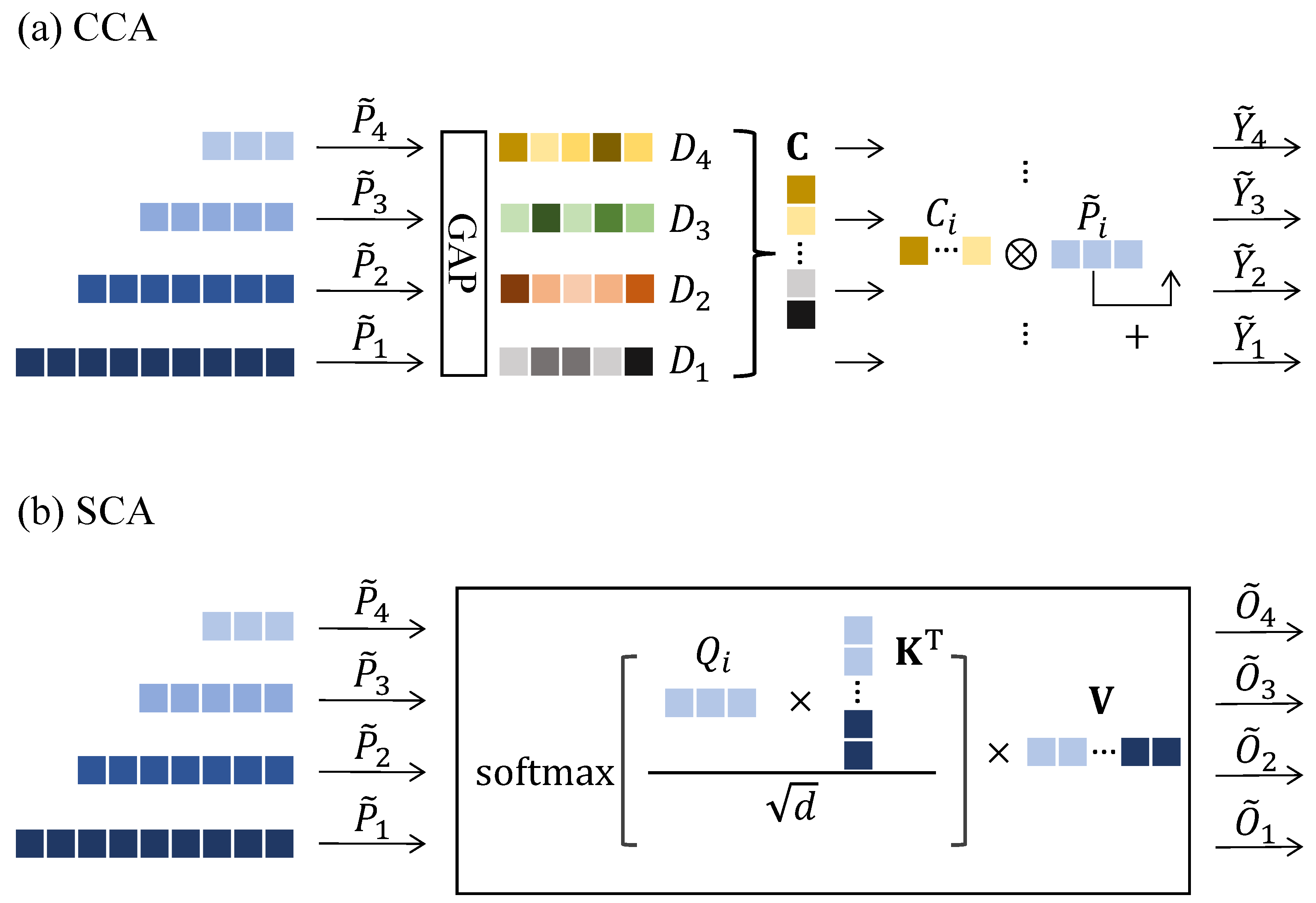
3.4.1. Channel Cross-Attention

Exploring feature channels has been very important in many vision tasks because feature channels encode visual patterns that are strongly related to foreground objects [10,53,59,70,71]. Many studies have been proposed to enhance the representational power of a network by explicitly modeling the interdependencies between the feature channels [72,73,74,75,76]. In the same vein, we propose CCA to further enhance the representational richness of multiscale patches by explicitly modeling their cross-scale channel interactions.

We illustrate CCA in Figure 3a. First, we apply global average pooling (GAP) to ${\tilde{P}}_i$ to obtain a global channel descriptor $D_i\in {\mathbb{R}}^{c_i}$ for each stage. The c-th element of $D_i$ is calculated by

$$D_i^c={\displaystyle \frac{1}{{\tilde{k}}_i}}\sum _{j=1}^{{\tilde{k}}_i}{\tilde{P}}_i^c\left(j\right),$$

(8)

where j is the patch index $j\in \{1,2,\cdots ,{\tilde{k}}_i\}$. From the stage-specific channel descriptors, we compute the channel attention score as follows:

$$\begin{array}{cc}\hfill & \mathbf{D}=\mathtt{concat}\left(D_1,D_2,D_3,D_4\right)\in {\mathbb{R}}^c,\hfill \\ \hfill & \mathbf{C}=\mathrm{sigmoid}\left(W^{c,1}\mathrm{ReLU}\left(\mathrm{BN}\left(W^{c,0}\mathbf{D}\right)\right)\right)\in {\mathbb{R}}^c,\hfill \end{array}$$

(9)

where $c=\sum c_i$, $W^{c,0}\in {\mathbb{R}}^{\frac{c}{2}\times c}$, and $W^{c,1}\in {\mathbb{R}}^{c\times \frac{c}{2}}$. We then split $\mathbf{C}$ back into $C_i\in {\mathbb{R}}^{c_i}$ and recalibrate the channels of ${\tilde{P}}_i$ as follows:

$${\tilde{Y}}_i={\tilde{P}}_i\otimes C_i+{\tilde{P}}_i,$$

(10)

where ⊗ indicates element-wise multiplication. In (9), we compute the channel attention score by aggregating the channel descriptors of all multiscale patches. It captures channel dependencies in a cross-scale way and reflects them back to each stage-specific piece of channel information.

3.4.2. Spatial Cross-Attention

In addition to channel-wise interactions, we can compute the spatial-wise interdependencies of selected multiscale patches. To this end, we propose SCA, which is a multiscale extension of MSA [19,28].

We illustrate SCA in Figure 3b. First, we compute query, key, and value tensors $Q_i$, $K_i$, $V_i$ for every ${\tilde{Y}}_i$,

$$Q_i={\tilde{Y}}_i{W}_i^Q,K_i={\tilde{Y}}_i{W}_i^K,V_i={\tilde{Y}}_i{W}_i^V,$$

(11)

where $W_i^Q$, $W_i^K$, $W_i^V\in {\mathbb{R}}^{c_i\times d}$, and $Q_i$, $K_i$, $V_i\in {\mathbb{R}}^{{\tilde{k}}_i\times d}$. After that, we concatenate the $K_i$ and $V_i$ of all stages to generate global key and value tensors $\mathbf{K}$, $\mathbf{V}$,

$$\begin{array}{cc}\hfill & \mathbf{K}=\mathtt{concat}\left(K_1,K_2,K_3,K_4\right)\in {\mathbb{R}}^{\tilde{k}\times d},\hfill \\ \hfill & \mathbf{V}=\mathtt{concat}\left(V_1,V_2,V_3,V_4\right)\in {\mathbb{R}}^{\tilde{k}\times d},\hfill \end{array}$$

(12)

where $\tilde{k}=\sum {\tilde{k}}_i$. Now, we can compute self-attention for $Q_i$, $\mathbf{K}$, $\mathbf{V}$, and a single linear layer is used to restore the dimension,

$$\begin{array}{cc}\hfill & {\tilde{A}}_i=\mathrm{Softmax}\left(Q_i{\mathbf{K}}^T/\sqrt{d}\right)\mathbf{V},\hfill \\ \hfill & {\tilde{O}}_i={\tilde{A}}_i{W}_i^s,\hfill \end{array}$$

(13)

where ${\tilde{A}}_i\in {\mathbb{R}}^{{\tilde{k}}_i\times d}$, $W_i^s\in {\mathbb{R}}^{d\times c_i}$, and ${\tilde{O}}_i\in {\mathbb{R}}^{{\tilde{k}}_i\times c_i}$. SCA is also implemented in a multihead manner [28]. For global key and value, SCA captures how strongly multiscale patches interact spatially with each other. Specifically, SCA models how large-scale semantic patches decompose into more fine-grained views, and conversely, how small-scale fine-grained patches can be identified in more global views.

3.5. Training

After the MSCA block, we can extract ${\overline{\mathtt{CLS}}}_i$ from ${\tilde{O}}_i$ and compute the class prediction $y_i$ using a linear classifier. In addition, we can compute $y_{con}$ by concatenating all ${\overline{\mathtt{CLS}}}_i$ tokens. For model training, we compare every $\mathbf{y}=\{y_1,y_2,y_3,y_4,y_{con}\}$ for the ground-truth label $\widehat{y}$,

$$\mathcal{L}=\sum _{y\in \mathbf{y}}\sum _{t=1}^n-{\widehat{y}}^{t}log{y}^t,$$

(14)

where n is the total number of classes, and t denotes the element index of the label. To improve model generalization and encourage diversity of representations from specific stages, we employ soft supervision using label smoothing [8,77]. We modify the one-hot vector $\widehat{y}$ as follows:

$${\widehat{y}}_{\alpha }\left[t\right]=\left\{\begin{array}{cc}\alpha \hfill & t=\widehat{t}\hfill \\ {\displaystyle \frac{1-\alpha }{n}}\hfill & t\ne \widehat{t}\hfill \end{array}\right.$$

(15)

where $\widehat{t}$ denotes index of the ground truth class, and $\alpha$ denotes a smoothing factor $\alpha \in [0,1]$. $\alpha$ controls the magnitude of the ground truth class. As a result, the different predictions are supervised with different labels during training. We set $\alpha$ to increase in equal intervals by $0.1$ from $0.6$ to 1, so $y_1$ has the smallest $\alpha =0.6$.

For inference, we conduct a final prediction considering all of $\mathbf{y}$,

$$y_{all}=\sum _{y\in \mathbf{y}}y,$$

(16)

where the maximum entry in $y_{all}$ corresponds to the class prediction.

4. Experiments

In this section, we evaluate our proposed M2Former on widely used fine-grained benchmarks. In addition, we conduct ablation studies and further analyses to validate the effectiveness of our method. More details are described in the following section.

4.1. Datasets

We use two FGVR datasets to evaluate the proposed method: Caltech-UCSD Birds (CUB) [1] and NABirds [50]. The CUB dataset consists of 11,788 images and 200 bird species. All images are split into 5994 for training and 5794 for testing. The NABirds is a larger dataset, consisting of 48,562 images and 555 classes. All images are split into 23,929 for training and 24,633 for testing. Most of our experiments are conducted on CUB.

4.2. Implementation Details

We use MViTv2-B [45] pretrained on ImageNet21K [78] as our backbone network. We add MSPS to every stage of MViTv2-B. After patch selection, selected patches pass through one MSCA block. We empirically set $\mathbf{k}=\{k_1,k_2,k_3,k_4\}$, the number of patches selected for each stage, to $\{6,18,54,162\}$. Our training recipe follows the same as recent work [18]. The model is trained for a total of 10,000 iterations, and an SGD optimizer with momentum of 0.9 and weight decay of 0 is used. The batch size is set to 16, and the initial learning rate is set to 0.03. The learning rate has a cosine decay schedule [79]. For augmentations, raw images are first resized into $600\times 600$, followed by cropping into $448\times 448$. We use random cropping for training, and center cropping for testing. Random horizontal flipping is adapted to training images. We implement the whole model with the PyTorch framework on three NVIDIA A5000 GPUs (NVIDIA, Santa Clara, CA, USA).

4.3. Main Results

We compare our M2Former with state-of-the-art FGVR methods, including ViT-based and CNN-based models on each dataset.

4.3.1. Results on CUB

First, the evaluation results on CUB are presented in

Table 1. Comparison with the state-of-the-art methods on CUB.

Method	Backbone	Accuracy (%)
RA-CNN [51]	VGG19	85.3
NTS-Net [80]	ResNet50	87.5
Cross-X [81]	ResNet50	87.7
DBTNet [55]	ResNet101	88.1
DF-GMM [62]	ResNet50	88.8
PMG [12]	ResNet50	89.6
GDSMP-Net [17]	ResNet50	89.6
API-Net [54]	DenseNet161	90.0
P2P-Net [8]	ResNet50	90.2
TransIFC+ [82]	SwinT-B	91.0
TransFG [18]	ViT-B	91.7
RAMS-Trans [21]	ViT-B	91.3
FFVT [22]	ViT-B	91.6
IELT [83]	ViT-B	91.8
ACC-ViT [84]	ViT-B	91.8
Dual-TR [85]	ViT-B	92.0
DCAL [20]	R50-ViT-B	92.0
M2Former (ours)	MViTv2-B	92.4

. As shown in Table 1, our M2Former obtained a top-1 accuracy of 92.4%, which significantly outperforms CNN-based methods. In particular, M2Former improves recent P2P-Net [8] by 2.2%. In addition, M2Former achieved higher accuracy compared with ViT-based models using SSPS. Specifically, M2Former outperforms TransFG [18], RAMS-Trans [21], FFVT [22], and DCAL [20] by 0.7%, 1.1%, 0.8%, and 0.4%, respectively. These results indicate that our proposed MSPS encourages enhanced representations compared with SSPS.

4.3.2. Results on NABirds

The evaluation results on NABirds are presented in

Table 2. Comparison with the state-of-the-art methods on NABirds.

Method	Backbone	Accuracy (%)
MaxEnt [87]	DenseNet161	83.0
Cross-X [81]	ResNet50	86.4
PAIRS [88]	ResNet50	87.9
API-Net [54]	DenseNet161	88.1
PMGv2 [86]	ResNet101	88.4
CS-Parts [89]	ResNet50	88.5
MGE-CNN [90]	ResNet101	88.6
GDSMP-Net [17]	ResNet50	89.0
FixSENet-154 [91]	SENet154	89.2
ViT [19]	ViT-B	89.9
IELT [83]	ViT-B	90.8
TransFG [18]	ViT-B	90.8
TransIFC+ [82]	SwinT-B	90.9
Dual-TR [85]	ViT-B	91.3
ACC-ViT [84]	ViT-B	91.4
M2Former (ours)	MViTv2-B	91.1

. Our proposed M2Former obtains the top-1 accuracy of 91.1% on NABirds. Compared with the CNN-based models, our M2Former shows significantly improved performance. For example, M2Former improves PMGv2 [86] by 2.7%. Compared with ViT-based models, our M2Former lags slightly behind Dual-TR [85] and ACC-ViT [84] but outperforms TransIFC+ [82], IELT [83], and TransFG [18]. In particular, M2Former improves TransFG [18] by 0.3%, which shows the effectiveness of MSPS compared with SSPS.

4.4. Ablation Study

We analyzed each component of the proposed M2Former through the ablation study. All experiments are conducted on the CUB dataset.

4.4.1. Ablation on Proposed Modules

We investigate the influence of the proposed modules (i.e., MSPS, CTT, CCA, SCA) included in the M2Former architecture. The results are presented in

Table 3. Effect of the proposed modules on CUB.

Index	MSPS	CTT	CCA	SCA	# Params.	Accuracy (%)
(a)					52M	91.6
(b)	✓				60M	91.6
(c)	✓	✓			62M	92.1
(d)	✓	✓	✓		64M	92.2
(e)	✓	✓		✓	64M	92.1
(f)	✓	✓	✓	✓	65M	92.4

. The pure MViTv2-B baseline obtained the top-1 accuracy of 91.6% on CUB (Table 3 (a)). When MSPS was added, we did not find any noticeable improvement (Table 3 (b)). This indicates that effectively incorporating selected patches into model decisions is more important than patch selection itself. For this purpose, CTT allows multiscale patch information to be shared across the entire network through transferred global CLS tokens. Indeed, with CTT, we improve the baseline by 0.5% (Table 3 (c)). In addition, CCA and SCA capture more direct interactions between multiscale patches, but using CCA or SCA alone was not effective for improvement (Table 3 (d) and (e)). On the other hand, when using both CCA and SCA (full MSCA block), we obtain the highest top-1 accuracy of 92.4%, which improves the baseline by 0.8% (Table 3 (f)). This means that the spatial-/channel-level interactions of multiscale patches are strongly correlated and need to be considered simultaneously.

4.4.2. Number of MSCA Blocks

Table 4. Effect of the number of MSCA blocks on CUB.

Num. Blocks	Accuracy (%)
1	92.4
2	92.1
3	92.2
4	92.2

shows the results of the ablation experiment on the number of our MSCA blocks. The results show that using a single MSCA block performs best and increasing the number of MSCA blocks no longer yields a meaningful improvement. This means that a single MSCA block is sufficient to model the interactions of multiscale patches. Moreover, using one MSCA block is efficient as it only introduces small extra parameters.

4.4.3. Number of Selected Patches

Table 5. Effect of the number of selected patches on CUB.

k	Accuracy (%)
{6, 8, 10, 12}	92.2
{6, 12, 24, 48}	92.2
{6, 18, 54, 162}	92.4
{7, 28, 112, 448}	92.1

shows the influences of the number of selected patches. We define it as $\mathbf{k}=\{k_1,k_2,k_3,k_4\}$, where $k_i$ is the number of patches selected through patch selection at stage i. $k_i$ is set differently for each stage. As shown in Table 5, the larger the overall number of selected patches, the better the performance in general. However, after it grows to some extent, increasing selected patches is insignificant and causes unnecessary computations. We empirically found the optimal $\mathbf{k}=\{6,8,54,162\}$.

4.4.4. Different Backbone Networks

In

Table 6. Comparison of different backbone networks on CUB.

Method	Accuracy (%)
CvT-21 [44]	89.3
CvT-21MSPS	90.0
SwinT-B [32]	90.6
SwinT-BMSPS	91.3

, we analyze whether our method provides consistent effects on different backbone networks. We use CvT-21 [44] and SwinT-B [32] as backbone architectures and compare them to their baseline. Both are initialized with pretrained weights from ImageNet21K [78]. The proposed modules are added to all three stages for CvT-21 and all four stages for SwinT-B. We follow the training recipe from recent work [18]. It should be noted that CTT could not be applied to the SwinT-B backbone, as it does not use a CLS token. In addition, SwinT-B uses an input resolution of $384\times 384$: raw images are first resized into $510\times 510$ followed by cropping into $384\times 384$. As shown in Table 6, Cvt-21 and SwinT-B baselines obtained top-1 accuracies of 89.3% and 90.6%, respectively. When we added the proposed modules, we could obtain top-1 accuracies of 90.0% and 91.3%, which are both 0.7% higher than their pure counterparts. This suggests that selecting multiscale salient patches and modeling their interactions is important for fine-grained recognition, and our method is beneficial for that purpose.

4.5. Further Analysis

In this section, we conduct additional experiments to further validate the effectiveness of our proposed methods. All experiments are conducted on the CUB dataset.

4.5.1. Contributions from CTT

In

Table 7. Comparison of different CTT methods on CUB.

Method	Accuracy (%)
global pool	91.5
simple attach	91.9
CTT w/1-MLP	92.1
CTT w/2-MLP	92.4

, we examine the contributions from CTT. First, we start by not using the CLS token. In this set-up, the patch sequence selected at each stage does not contain any CLS tokens. Instead, selected patches that pass through the MSCA block are projected as feature vectors with global average pooling (GAP), and the features are used for final prediction through a linear layer. This is noted as the ‘global pool’ in Table 7. As a result, the global pool obtains a top-1 accuracy of 91.5%, which lags behind the MViTv2-B baseline (91.6% in Table 3). We conjecture that this low accuracy is due to the lack of a shared intermediary (i.e., CLS token) to aggregate the information of the selected multiscale patches, even when using the MSCA block.

Then, we initialized the CLS token of the backbone, and the patch sequence selected in each stage was concatenated with the CLS token of the same dimension that was detached before patch selection (as in Section 3.3 (4)). This is simply reattaching the CLS token that was detached before MSPS, so it is noted as ‘simple attach’ in Table 7. As a result, the simple attachment obtains an accuracy of 91.9%, which improves the global pool by 0.4%. We argue that this improvement comes from that simple attach can share information between multiscale patches through the CLS tokens. Since the global CLS token is detached with different channel dimensions at each stage, stage-specific patch information can be shared through the global CLS token to generate richer representations.

As discussed in Section 3.3, we propose CTT to enhance multiscale feature sharing. In this setup, each stage uses a ’transferred’ global CLS token rather than a simply ’detached’ one. This can be implemented using a single projection layer to match its dimensions (noted ‘CTT w/1-MLP’ in Table 7). As a result, it obtains an accuracy of 92.1%, which improves the simple attach by 0.2%. Compared with using a detached CLS token at an intermediate stage, transferring the globally updated CLS token is more effective in that it can inject local information of each stage into the object’s deep semantic information, utilizing the same representational power of the network. Finally, CTT performs best when using 2-layer MLP with nonlinearity (noted ‘CTT w/2-MLP’ in Table 7).

4.5.2. Contributions from MSPS

In the earlier section, we pointed out that SSPS is suboptimal because it is difficult to deal with scale changes. We now show that our proposed MSPS can consistently improve performance on different object scales.

First, we need to classify a given set of objects according to their scale. Following COCO [92], we categorize all objects into large, medium, and small-sized objects according to their bounding box size. We compute the size of the bounding box using the given box coordinates and sort them in ascending order. Then, we compute the quartiles for sorted bounding box sizes. Finally, we classify an object as a small-sized (ob_s) object if its bounding box size is less than the first quartile, as a large-sized object (ob_l) if its bounding box size is greater than the third quartile, and as a medium-sized (ob_m) object otherwise. Specifically, 25% of the objects are small, 50% are medium, and 25% are large. Example images for each category are shown in Figure 4.

We train five model variants with different MSPS stages: M2Former_none, M2Former₄, M2Former_3,4, M2Former_2,3,4, M2Former_full. It should be noted that M2Former_none is exactly the same as the MViTv2-B baseline. For comparison, we trained TransFG [18], which conducts SSPS at the last encoder block.

The results are presented in

Table 8. Comparison of different MSPS stages on CUB.

Method	Stages for Patch Selection				Accuracy (%)
	Stage1	Stage2	Stage3	Stage4	obl	obm	obs	Total
TransFG [18]	SSPS at Last Block				91.7	91.7	90.1	91.3
M2Formernone					92.3(+0.6)	91.8(+0.1)	90.5(+0.4)	91.6(+0.3)
M2Former4				✓	91.9(+0.2)	91.7(+0.0)	90.6(+0.5)	91.5(+0.2)
M2Former3,4			✓	✓	92.9(+1.2)	91.9(+0.2)	90.8(+0.7)	91.9(+0.6)
M2Former2,3,4		✓	✓	✓	92.9(+1.2)	92.4(+0.7)	91.4(+1.3)	92.3(+1.0)
M2Formerfull	✓	✓	✓	✓	92.9(+1.2)	92.6(+0.9)	91.4(+1.3)	92.4(+1.1)

. First, TransFG obtained a total top-1 accuracy of 91.3%, which obtained accuracies of 91.7% for ob_l, 91.7% for ob_m, and 90.1% for ob_s. The performance of ob_s seems to lag behind ob_l and ob_m. M2Former_none obtains a total top-1 accuracy of 91.6%, which outperforms TransFG by 0.3% higher. This means that we can achieve satisfactory results simply by using MS-ViT. Additionally, the improvement was prominent in ob_l and ob_s (0.6% and 0.4% higher, respectively), indicating that multiscale features are important in mitigating scale variability.

When we add MSPS to stage-4 (M2Former₄), we obtain a top-1 accuracy of 91.5%, which is 0.2% higher than the baseline. M2Former₄ is almost identical to SSPS, as it selects only single-scale patches in a single stage. However, M2Former₄ obtained a lower total top-1 accuracy than M2Former_none, and it generally results in lower accuracy at all scales. This is also in contrast to previous findings [18], where performance was improved when patch selection was conducted at the last block.

However, when adding the MSPS in stage-3 (M2Former_3,4), we obtained a top-1 accuracy of 91.9%, which outperforms the SSPS baseline by 0.6%. The improvements were found at all object scales but were noticeable at ob_l (1.2% higher compared with the SSPS baseline). This means that salient patches from stage-3 (along with selected patches from stage-4) provide the definitive cue for large objects.

We can see this improvement even when adding MSPS in stage-2 (M2Former_2,3,4). In particular, adding MSPS in stage-2 leads to improvements for ob_m and ob_s. Compared with the SSPS baseline, it is 0.7% higher for ob_m, 1.3% higher for ob_s, and 1.0% higher for total accuracy. This indicates that the finer-grained object features extracted at stage-2 enhance representations for small/medium-sized objects.

Finally, when adding MSPS to stage-1 (M2Former_full), we obtained the highest total top-1 accuracy of 92.4%, with a slight further improvement in ob_m. In summary, MSPS from high to low stages models a feature hierarchy from deep semantic features to subtle fine-grained features, which consistently improves recognition accuracy for large to small-sized objects. As a result, MSPS encourages networks to generate richer representations of fine-grained objects and to be more flexible to scale changes.

4.6. Qualitative Analysis

To further investigate the proposed method, we present the visualization results in Figure 5 and Figure 6.

Figure 5 shows the selected patches at each stage by conducting MSPS for several images sampled from CUB. In each subfigure, the first column is the original image, and selected patches from stage-4 to stage-1 are marked with red rectangles. At higher stages, large-sized patches that capture several parts of the object are selected. Sufficiently large patches are appropriate for modeling the intraimage structure and overall semantics of a given object. On the other hand, at the lower stage, smaller patches are chosen to model subtle details. In particular, the smallest size patches selected in stage-1 capture the coarsest features, such as object edges. As a result, MSPS enhances object representations at different levels for each stage.

Figure 6 shows the cross-attention maps of MSCA for selected patches. For visualization, we sample some patches selected from stage-4. And then, we extract cross-attention maps between sampled patches and patches selected at different stages from SCA. In Figure 6, the first column shows the sampled stage-4 patch as a red rectangle. The second to fourth columns show the attention maps between sampled patches and selected patches from stage-3 to stage-1 as orange rectangles. The brightness of a color indicates the strength of attention: brighter means stronger interactions. In addition to modeling channel interactions in CCA, SCA models spatial interactions between selected multiscale patches. As a result, each selected patch can be correlated with other patches that exist in different locations at different scales.

5. Conclusions

In this paper, we propose a MultiScale Patch Selection (MSPS) for fine-grained visual recognition (FGVR). MSPS selects salient patches in multiscale at each stage of a MultiScale Vision Transformer (MS-ViT) based on mean activation. In addition, we introduce Class Token Transfer (CTT) and MultiScale Cross-Attention (MSCA) to effectively deal with selected multiscale patch information. CTT transfers the globally updated CLS token to each stage so that stage-specific patch information can be shared throughout the entire network. MSCA directly models the spatial-/channel-wise correlation between selected multiscale patches. Compared with Single-Scale Patch Selection (SSPS), MSPS provides richer representations for fine-grained objects and flexibility for scale changes. As a result, our proposed M2Former obtains accuracies of 92.4% and 91.1% on CUB and NABirds, respectively, which outperform CNN-based models and ViT-based SSPS models. Our ablation experiments and further analyses validate the effectiveness of our proposed methods.