Camera Calibration in High-Speed Robotic Assembly Operations

Featured Application

The presented methodology can be used in all robotic assembly tasks where the camera position changes during operation, such as tasks where the camera is mounted on the robotic arm near the end-effector—for example, in fuse box assembly applications.

Abstract

The increase in positioning accuracy and repeatability allowed the integration of robots in assembly operations using guidance systems (structured applications) or video acquisition systems (unstructured applications). This paper proposes a procedure to determine the measuring plane using a 3D laser camera. To validate the procedure, the camera coordinates and orientation will be verified using robot coordinates. This procedure is an essential element for camera calibration and consists of developing a mathematical model using the least square method and planar regression. The mathematical model is considered necessary as a step towards optimizing the integration of robotic vision systems in assembly applications. A better calibrated camera has the potential to provide better recognition results, which are essential in this field. These improved results can then be used to increase the accuracy and repeatability of the robot.

1. Introduction

Over the last several decades, robotics grew continuously and positioned itself as one of the most dynamic fields in engineering. Today, different areas in robotics are more and more integrated together into the same applications. Industrial robots, once reprogrammable machines that were only capable of performing repetitive tasks again and again, are now able to use a large variety of sensors to collect data from the working environment and can make decisions based on the information received. The sensors used in industrial robotics include (but are not limited to) force and torque sensors, LIDAR sensors, ultrasonic sensors, infrared sensors, laser sensors, capacitive sensors, temperature sensors, gyroscope, accelerometers, and cameras. The growing level of sensor integration allowed a greater level of interaction between the industrial robots and the nearby equipment, as well as program adaptability and better responses to changes and various events in the working environment. This, in turn, increased the flexibility of industrial robotic systems [1]. Benefiting from growing levels of sensor integration, industrial robots gained better capabilities and were increasingly integrated into automated lines for palletizing, sorting operations, or automating simple, repetitive tasks [2]. Actually, this direction of evolution in industrial robotics represents a response to the requirements of IoT and Industry 4.0, concepts that dictate the general trend in today’s industrial landscape. Smart robots that are capable of operating in uncertain environments (that is, environments that are not deterministic) are required in many modern tasks [3].

Being the backbone of this approach in robotics, sensors are present in virtually every industrial robotic application. They are essential for interaction with the working environment, for M2M (machine-to-machine) communication, and for monitoring the internal state of the robotic system. One of the most important areas in the field of industrial robotics, collaborative applications, benefits from the extensive use of sensors. Sensors are also the base of the transition towards smart manufacturing and Cyber-Physical Systems (CPS) as solution to full development of smart factories. Being the main elements for data acquisition, sensors allow collecting information and gaining knowledge, which, in turn, represent the building blocks for training artificial intelligence systems and big data analysis [4].

One of the main issues in uncertain working environments is linked to unknown part position, orientation, dimensions, and shape. In an industrial application, creating a deterministic setup for the workobject often requires fixtures, guiding elements, or other pieces of equipment that increase the costs and complexity. Furthermore, working with known part dimensions and shape imposes limitations on application flexibility. Being able to work with parts that have random positions and orientations, while allowing for large variations in dimensions and shape, greatly improves flexibility and productivity, and represents an important step towards smart manufacturing. Robotic vision systems are among the solutions that address these issues. These systems include cameras that, together with specific software (ifm vision assistant version 2.6.24), process digital image data in order to provide information to the manufacturing system. Besides object recognition, robotic vision systems have multiple uses, such as defectoscopy, object tracking, pattern recognition, augmented reality, and optical character recognition (OCR), and can be integrated with AI and machine learning [5,6].

Taking these aspects into account, from the robotic task point of view, the vision system has the potential to increase productivity, the flexibility of the application, and the collaborative level, as well as the accuracy and repeatability of the robot. The increase in positioning accuracy and repeatability allows the integration of robots in assembly operations using guidance systems (structured applications) or video acquisition systems (unstructured applications) [1]. In the case of the guidance systems, the assembly requires the existence of additional stages of guiding and repositioning the assembled landmarks, stages that entail additional times and, implicitly, a reduction in productivity. Unlike structured applications, unstructured applications (e.g., Pick and Place applications) require the existence of a video camera system capable of identifying workobject shape and position and transmitting the coordinates to the robotic assembly systems. In this case, robots with compliant systems are used to carry out the assembly and video systems are used to check the positioning accuracy. Industrial robots used in automated production lines are programmed to use predefined trajectories for assembly operations [2,3]. Using this programming method, robots can work with high precision, but they cannot prevent any unforeseen changes in the position of the manipulated components.

These disadvantages can be corrected by integrating a robot vision system. Typically, industrial vision systems are mounted outside the working area in a predefined position and focus on a well-defined task such as measuring a gap, checking the correct position of a part, pattern recognition, detecting various surface defects, etc. This approach has several disadvantages, such as a limited field of view in certain assembly operations when the view is obstructed by the robot. Additionally, different tasks may require different cameras or different camera types, and, sometimes, it is necessary to move the robotic arm to clear the camera’s field of view. Some of these disadvantages can be eliminated by using a mobile camera mounted on the robotic arm. This way, the robot arm is not obstructing the camera’s field of view, and image acquisition can be performed when the robot moves along working paths. Using this approach, the assembly total time could be greatly improved. The only drawback of this method is related to the camera accuracy and calibration. Usually, camera calibration is performed before every measurement task.

As previously mentioned, vision systems are particularly valuable in applications that are most likely to include uncertainties regarding part shape, position, and orientation. 3D cameras are more likely to be encountered in robotic tasks such as assembly or pick and place. Niu et al. [7] presented the case of a pocket calculator assembly process. The vision system is used to identify the part position and ensure the reliable picking of components and correct placement within the assembly. Using the camera software, the coordinates of each component are extracted as it enters the workspace. For component placement within the assembly, the system compares the current coordinates of each part to the required coordinates and computes the offset.

Vision systems are also widely used in mobile phone assembly. In a study by Song et al. [8], an application involving a camera mounted on a robot arm was explored. The assembly process was divided into four stages: camera calibration, part identification, picking, and placement. Components were delivered via a conveyor belt, with parts randomly positioned. After calibration, the camera was employed to determine the position and orientation of each workpiece using coordinate systems and offsets. The vision system also facilitated part placement within the assembly by utilizing object recognition and minimum rectangle fitting techniques.

Accurate calibration ensures precise measurements and reliable analysis by correcting distortions. Camera calibration refers to both the intrinsic and extrinsic calibration. Intrinsic calibration determines the optical properties of the camera lens, including the focal point, principal point, and distortion coefficients [9], while extrinsic calibration refers to the camera orientation concerning the measuring plane. Intrinsic calibration can be performed once for each use of the camera. However, when using moving cameras, the main challenge is determining the actual camera position relative to the measuring plane.

Regarding the characteristics of the robots used in assembly applications, two of the most important parameters are accuracy and repeatability. It should be taken into account that most assembly operations are performed by articulated arm or SCARA robots. For these robot types, repeatability is typically around 0.01–0.02 mm. While, in most cases, the accuracy value is not published by the producers, robotic assembly operations generally require it to be around 0.2–0.3 mm.

This article proposes a procedure to determine the measuring plane using a 3D laser camera. For validation purposes, the camera coordinates and orientation will be verified using robot coordinates. This procedure is an essential element for camera calibration. The development of the presented procedure was considered necessary as a step towards optimizing the integration of robotic vision systems in assembly applications. A better calibrated camera has the potential to provide better recognition results, which are essential in this field. These improved results can then be used to increase the accuracy and repeatability of the robot.

The article is structured as follows:

• Section 1 presents the scientific context, the main goal of the research, and the importance of the studies aspects in the field of robotic manufacturing systems.
• Section 2 presents the state of the art in the field of camera calibration for robotic vision systems.
• Section 3 presents the materials and methods used for research, including the methods used, the experimental setup and procedure, and the implemented calculation algorithms.
• Section 4 presents the measurement results, and the calculation outputs, followed by a discussion that validates the experimental results.
• Section 5 presents the conclusions that highlight the main results and contributions of the research.

2. State of the Art

Industry 4.0 represents the ongoing stage of macro-industrial development. Historically, each industrial development stage was powered by a huge leap in a certain scientific field: Industry 1.0 was triggered by mechanical devices and steam power, Industry 2.0 was triggered by electricity, and Industry 3.0 was triggered by electronics [9]. Following the same trend, Industry 4.0 was triggered by software and networking development. The manufacturing systems and the robots themselves are evolving on the “smart” path, being more and more capable of solving certain issues and adapting to significant changes on their own. On the other hand, the trend is to facilitate human integration in the industrial environment, somewhat reversing the long-standing status of industrial robots as machines that replace human work. This aspect is illustrated by the growing segment of collaborative applications [10,11,12,13,14]. Industry 4.0 is based on sensors, M2M communication, networking, ML, and, more recently, AI.

As an important element in the sensors ecosystem, robotic vision has been approached by a large number of research works. An interrogation on Google Scholar returned more than 17,000 results published since 2020. One of the most important issues in the field is linked to camera calibration, as shown by [15,16,17,18,19,20]. Camera calibration is performed in order to establish a link between the captured image coordinates and an external reference, such as the coordinates of the application or the coordinates of the robot workspace. Defining this relationship is necessary in order to develop a framework that can be used to convert coordinates from one reference to another. This is essential for acquiring relevant geometric information from the work scene, including workobject characteristics. Furthermore, using such a framework ensures that the collected data are transposed into a format that can be used outside of camera (image) frame of reference [21].

A comprehensive study of the relevant scientific literature revealed several methods and approaches regarding camera calibration in robotic vision applications. Wang et al. [15] identified three groups of parameters that should be calibrated: camera parameters, hand-eye parameters, and structured light plane parameters. The research used a planar checkerboard as the calibration plane. Considering the robot base and tool coordinate systems as well as the camera coordinate system, the algorithm uses homogenous transformation matrices to determine the intrinsic and extrinsic parameters of the camera. For camera parameters calibration, the workpiece pose is changed several times while the robot-held camera is stationary. Then, the camera is moved to several different poses while the workobject remains stationary. Using the data collected through the experimental procedure, the hand-eye relation was determined as a homogenous transformation matrix. Furthermore, the plane equation for the measured points expressed in the robot base coordinate system was determined using the least square fitting.

$${}_C{}^{E}M=\left(\begin{array}{cc}R& T\\ 0& 1\end{array}\right)$$

(1)

The ultimate goal of any camera calibration and detection algorithm is to correctly recognize patterns, features, shapes, and other data in a format that can be further used in a broader context. Chang W.-C. and Wu C.-H. [22] proposed an iterative closest point algorithm approach to compare the object point cloud to a model point cloud and to perform the transformation using several iterations. The studied robotic task belonged to the bin-picking category. Matrix calculation based on homogenous transformation is used. The method assumes that the shape of the work object is known from the beginning and does not vary. Thus, a model of the part can be structured and used as a reference. The only variables remaining in the task environment are linked to the part position and orientation. For calibration purposes, a checkered board is used, as previously. The distance between the camera and the measurement plane is then determined using a point in the image plane p_I with a scale factor l, the intrinsic matrix of the camera K, the transformation matrix from the measurement plane frame to the image frame T, and the corresponding point in the measurement plane p_M.

$$\lambda p_I=KT{p}_M$$

(2)

Robotic vision is also an essential tool in surgical applications, where robot precision is the single most important parameter. Roberti et al. [23] developed a novel calibration technique using a da Vinci Research Kit robot. The method does not depend on the placement of the calibration board within the robot workspace. Also, the calibration of the robot kinematic structure is separated from the camera calibration. While using homogenous transformation matrices for calculations, as shown above, the calibration board has several points distributed in a circular pattern. Thus, the calibration approach is based on polar coordinates. By knowing the center of the set of acquired points and the radius of the circle over which the points are distributed, the pose of every calibration point is determined with respect to the camera. The best fitting plane is determined by using the centroid of the set of points c (with the points denoted as p) and the normal vector n, with the optimal estimations calculated as below.

$$\left\{\widehat{c},\widehat{n}\right\}={argmin}_{c, {\left|n\right|}_2=1}\sum _{i-1}^n{\left({\left(p_i-c\right)}^{T}n\right)}^2$$

(3)

Hernandez L. R. R. et al. [24] outlined the problems occurring when using cameras, among which is lens distortion. Due to this phenomena, straight lines appear as curvatures in the image, as shown in Figure 1.

The research performed by Hernandez L. R. R. et al. focused on Stereo Vision Systems (SVS) by using two cameras for detection. The main reasons for accuracy loss in these systems were identified as image digitalization and lens distortion. In this case, a board with 63 points distributed in a grid pattern was used. The test points were illustrated as crosses on the board. The camera calibration was performed by estimating the horizontal and vertical angles for each cross. Then, the information regarding these angles was extracted from each camera. Using the estimated angles, the adjustment angles were determined using the least square method. Then, the angles provided by the cameras were modified by the adjustment angles to compensate for errors.

Many research works dealing with camera calibration for robotic vision systems are based on the method presented by Zhang, Z [25]. This approach established a set of guidelines that were followed by many studies afterward [26,27,28,29,30,31,32,33]. The Zhang algorithm is based on a planar pattern used for calibration. To provide sufficient input data, the pattern must be presented to the camera in different (at least two) orientations. The method uses points in the measurement plane that are projected on the image plane. Then, the intrinsic and extrinsic parameters of the camera are determined through matrix calculation. The results are then refined through maximum likelihood inference. The radial distortion is compensated through a set of coefficients obtained through the linear least squares method.

One of the main disadvantages of the Zhang method—and subsequently, of all methods based on that one—is the requirement of a planar calibration pattern. Although the pattern is easy to create, it is still required. Furthermore, this approach makes the calibration process a separate task that requires the robot to interrupt the application in order to perform the calibration. The solution proposed by this study bypasses this issue by developing a calibration procedure that can be performed in real-time as a part of the application performed by the robot.

3. Materials and Methods

The study develops an algorithm for camera calibration in applications that implement robotic vision. The main objective of the proposed algorithm is to mathematically determine the measurement plane for the vision camera. The coordinates of the determined plane are then expressed in relation to robot coordinates. The required data are collected through experimental measurement.

The experimental setup uses an xArm (UFACTORY, Guangdong, China) collaborative robot with 5 DOF. A video processing unit (O3R222 from IFM, Essen, Germany) with 2 camera types was mounted on the robot using a custom mechanical interface. The video unit is illustrated in Figure 2.

The processing unit is based on a Dual-Core NVIDIA Denver 2 64-Bit; ARM Cortex A57 with a NVIDIA Pascal 256 CUDA Cores (1.3 TFLOPs) GPU and an Nvidia Jetson TX2 4GB Module. Both cameras can capture 2D and 3D images with different fields of view. Using a camera with 2D and 3D capabilities is required for the procedure since the 2D feature is used to capture the image itself, while the 3D feature is used to determine the distance to the measurement points. The 3D camera uses a PMD 3D chip which uses the ToF (Time of Flight) technology to measure the distances. The ToF sensor emits an infrared-modulated light that is reflected by surrounding surfaces. By measuring the time difference between the emitted and the response light, a distance is determined with high accuracy. The representation of a 3D camera consists of a point cloud in which each pixel’s color represents the distance to the first object encountered, as shown in Figure 3.

The accuracy of this camera model is highly dependent on the distance to the target. At distances under 1 m, the repeatability is less than 7 mm. Between 1 and 2 m, the accuracy decreases to 15 mm, and at distances beyond 4 m, it can reach up to 51 mm. Measurement repeatability can be significantly improved by using light filters. For camera calibration, a repeatability of less than 10 mm is considered acceptable.

The control software for the robot and the camera software were installed on separate laptops for more convenient operation. The experimental setup is illustrated in Figure 4. The purpose of the experimental setup is to determine the position and orientation of the camera relative to the measuring plane. To achieve this goal, a blank sheet of paper was used as a marker for the measuring area.

The main purpose of the study is to determine the position and orientation of a mobile camera relative to the plane on which the detected objects are placed. Once the position and orientation are determined, the calibration error due to perspective deformation can be compensated. Considering these aspects as well as the main goal of the research, the experimental procedures were conducted without any work objects placed in the testing area.

The calibration procedure employed two mathematical approaches to establish the relationship between the measurement plane and the camera’s frame of reference. The first approach focused on determining the rotation angles between the measurement plane and the camera’s XY plane. The second approach involved calculating the distance between the camera and a set of points on the measurement plane, followed by determining the plane through interpolation of these points.

For each approach, a mathematical model for determining the orientation of the camera relative to the measurement plane was developed. In each case, the mathematical model was tested and validated using the experimental setup. For the first approach, the procedure was structured into the following steps:

• Starting from the zero orientation, the camera was rotated with an arbitrary angle.
• The center of the image represents the origin of the image frame of reference. Using this coordinate system, a set of two points were chosen along the X axis and another set of two points was chosen along the Y axis—for the purpose of this research, these points were designated as measurement points. The points placed along the X axis were positioned symmetrically relative to the axis origin. The points placed along the Y axis were also in a relation of symmetry. The procedure was repeated until a total of four pairs of points were placed along the X axis, and another four pairs of points were placed along the Y axis. The points were placed along the axes considering the distance from the origin expressed in pixels, as indicated by the camera software. Thus, for the first pair, each point was placed at a distance of 20 pixels from the origin, one in the positive direction and one in the negative direction. For the second pair, the distance was 30 pixels. For the third pair, the distance was 40 pixels. For the fourth pair, the distance was 50 pixels. The pairs were placed in the same way along both the X and Y axis, as shown in Figure 4.
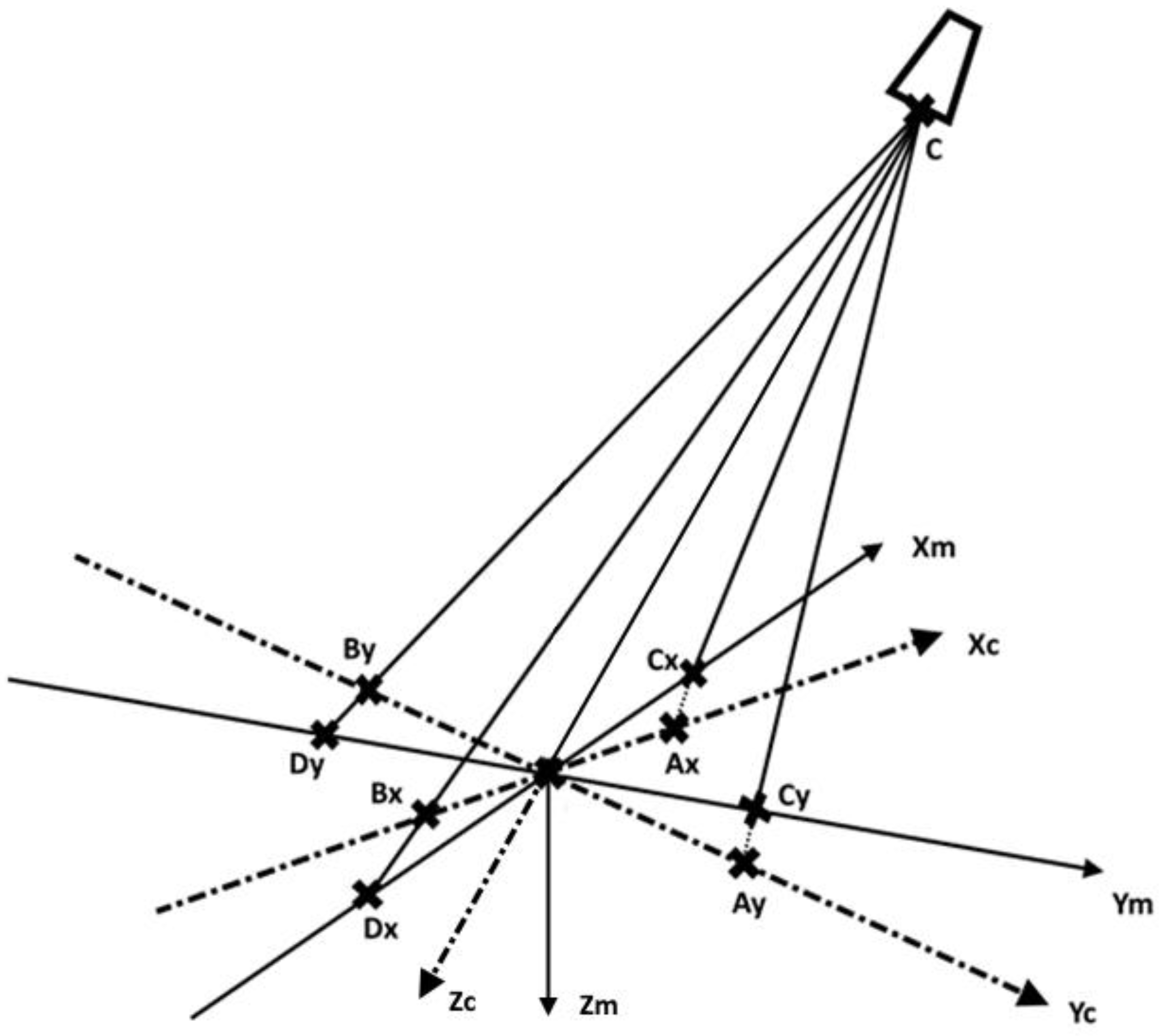
• Figure 5 shows all triangles in which the law of cosines was applied. C represents the camera focal point. The X_c and Y_c axes represent the camera coordinate system projected onto the measurement plane. The X_m and Y_m axes represent the coordinate system of the measurement plane. Both coordinate systems have the same origin O. C_x and D_x are the measurement points along the X_m axis, while A_x and B_x are the corresponding points along the X_c axis (the points in which the distances from C to the measurement points C_x and D_x intersect the X_m axis). Points C_y, D_y, A_y, and B_y have similar roles with respect to axes Y_m and Y_c.

  Figure 5. Camera calibration—first approach.

  Figure 5. Camera calibration—first approach.

• The distance from the camera to each measurement point was determined using the camera software. The first set of measurement points (the two pairs positioned at a distance of 20 pixels from the origin along the X and Y axes) and the camera position relative to the measurement plane are illustrated in Figure 4. The Xc and Yc axes belong to the camera reference frame. The Xm and Ym axes belong to the measurement plane reference frame.
• This approach is based on the law of cosines in order to determine the camera rotation angles around the X and Y axes relative to the measurement plane. The law of cosines determines a triangle when all the sides or two sides and the included angle are known. The general formula has the following form, with respect to Figure 4, considering the COC_y triangle:

  $${{CC}_y}^2={CO}^2+{{OC}_y}^2-2CO\ast {OC}_y\ast cos\propto$$

  (4)

  where $\propto$ is the angle between CO and OC_y.
• For the studied approach, the rotation around the X and Y axes can be considered separately. Thus, for the rotation around the X axis, the angle of rotation can be determined using the OCA_y triangle, as shown in Figure 6.

  Figure 6. Calculus plane.

  Figure 6. Calculus plane.

Since CA_y, CO, and OA_y are known from the camera software, $\propto$ can be determined by applying the law of cosines in the OCA_y triangle. The same method can be applied in the case of the rotation angle around the Y axis.

$$\propto =arccos{\displaystyle \frac{{CO}^2+{OA}_y^2-{CA}_y^2}{2\ast CO\ast {OA}_y}}$$

(5)

• Using this formula, the angle of rotation was determined for all pairs of points. The results were validated using the experimental setup described above by comparing the angle determined through the law of cosines with the actual rotation angle of the camera. Furthermore, the measurements were performed at three different heights chosen randomly.

For the second approach, the procedure was structured into the following steps:

• The initial orientation of the camera (“zero orientation”) was considered with the Z axis in the vertical position—parallel to the Z axis of robot’s base coordinate system.
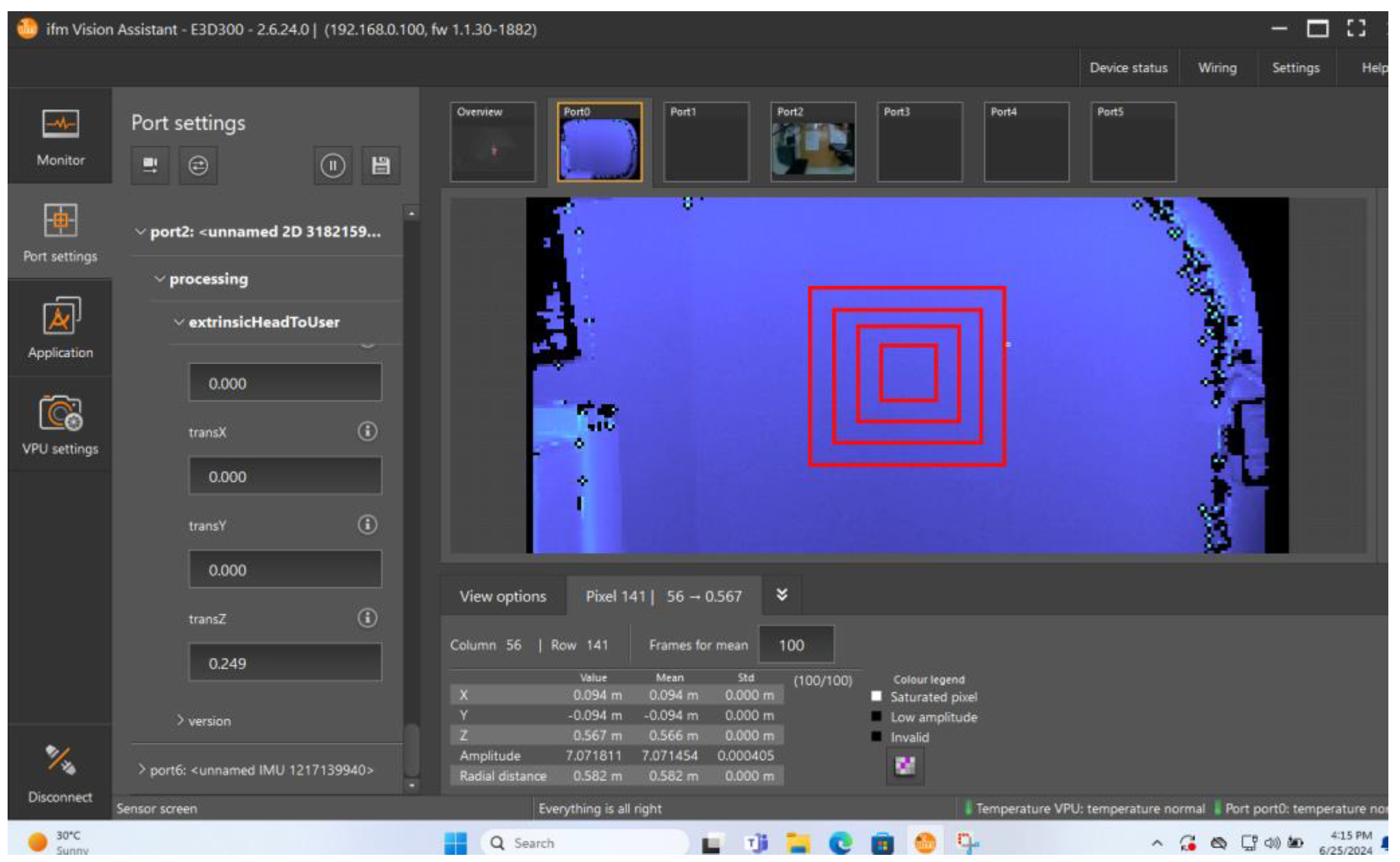
• The goal of the study is to determine the camera position and orientation relative to the measurement plane. During a real robot application, the orientation of the camera is not known and must be determined to perform the calibration. However, to validate the calibration method proposed in this article, the camera was inclined at a pre-determined angle of 80^o relative to the measurement plane around the Y axis.
• Using the image captured by the camera, a number of four rectangular measurement perimeters were considered as placed over the image. The measurement perimeters were concentric and centered on the origin of the image coordinate system. The dimensions of the measurement shapes were considered in pixels, as the building units on which the image structure is based. The dimensions of the measurement perimeters were 2 × 20 pixels, 2 × 30 pixels, 2 × 40 pixels, and 2 × 50 pixels. The perimeters placed over a captured image are illustrated in Figure 7. To compare both methods proposed in this paper, a single set of values was acquired using the camera’s proprietary software. In the figure, the camera software interface is shown. The image acquired by the camera is displayed in the central area of the interface. The measurement perimeters were represented upon the acquired image as red rectangles. Using a single set of points, both methods used the same input values.

  Figure 7. Measurement perimeters represented upon the acquired image.

  Figure 7. Measurement perimeters represented upon the acquired image.

• For each measurement perimeter, a number of nine measurement points were considered: the corners of the perimeter, the sides’ middle points, and the center of the rectangle. The distribution of the measurement points with respect to the image frame of reference is illustrated in Figure 8.

  Figure 8. The measurement points represented relative to the image frame of reference.

  Figure 8. The measurement points represented relative to the image frame of reference.

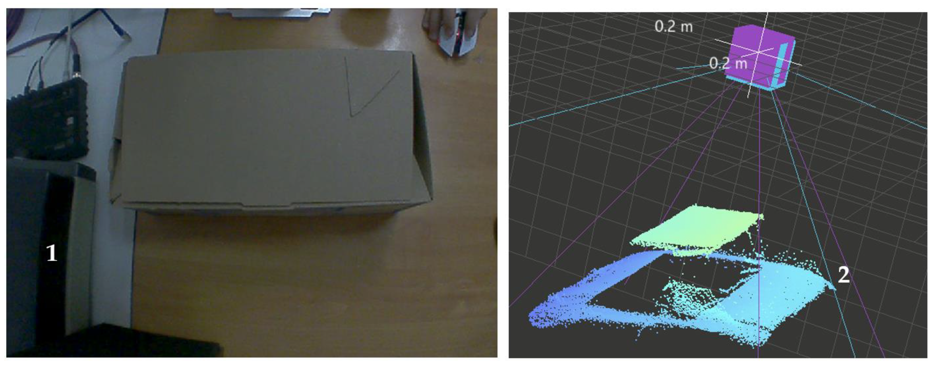
• The distance from the camera to each measurement point was determined using 3D data. The values were expressed with respect to the camera frame of reference

For the second approach, the following steps were performed:

• The initial orientation of the camera was maintained along with all nine measurement points previously described.
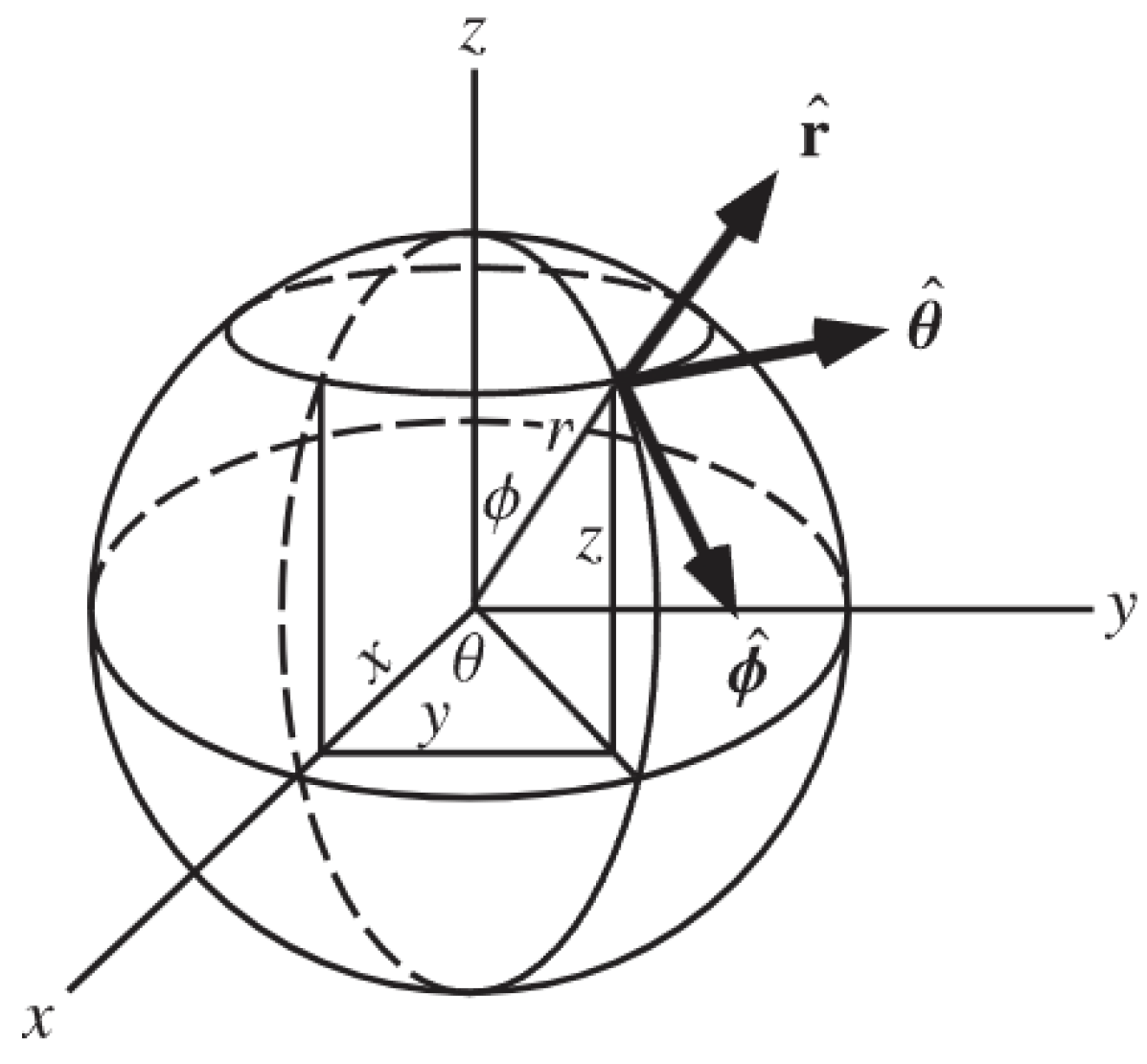
• A new spherical coordinate system was considered, and all nine measuring points were defined using the newly created reference system. In this spherical reference system, the first two coordinates, Theta and Phi, are computed based on the point position and the last one R is the distance acquired by the 3D camera. The center of the spherical coordinate system is represented by the camera focal point. The correlation between the spherical and Cartesian coordinates is shown in Figure 9.

  Figure 9. Correlation between spherical and Cartesian coordinates.

  Figure 9. Correlation between spherical and Cartesian coordinates.

• The Theta angle is computed using the point distribution relative to the camera sensor plane, as shown in Figure 10. As an example, for P1 the Theta angle is 45°.

  Figure 10. Point positioning in the camera sensor plane.

  Figure 10. Point positioning in the camera sensor plane.

• The Phi angle was determined using the camera resolution and the maximum angle for each direction. For P4, P5, and P6, the angle is determined in the X plane, while P2, P5, and P8, are determined in the Y plane. As P4 and P6 are symmetrical in the camera plane, the two angles are equal and the angle for P5 is 0, as illustrated in Figure 11.

  Figure 11. Phi and R coordinates of the spherical systems for P4, P5, and P6.

  Figure 11. Phi and R coordinates of the spherical systems for P4, P5, and P6.

• For P1, P3, P7, and P9, Phi angles were calculated considering OP5, a common leg (height) for all three right triangles (as seen in Figure 12) where angles P2OP5 and P4OP5 are the ones determined in the previous phase. The values for Theta and Phi angles are summarized in

  Table 1. Theta and Phi for calculation points.

  Point	Theta [°]	Phi [°]
  P1	45	7.32332
  P2	90	5.02232
  P3	135	7.32332
  P4	0	5.35714
  P5	0	0
  P6	180	5.35714
  P7	315	7.32332
  P8	270	5.02232
  P9	225	7.32332

  .

  Figure 12. Phi angle calculations for P1, P3, P7, and P9.

  Figure 12. Phi angle calculations for P1, P3, P7, and P9.
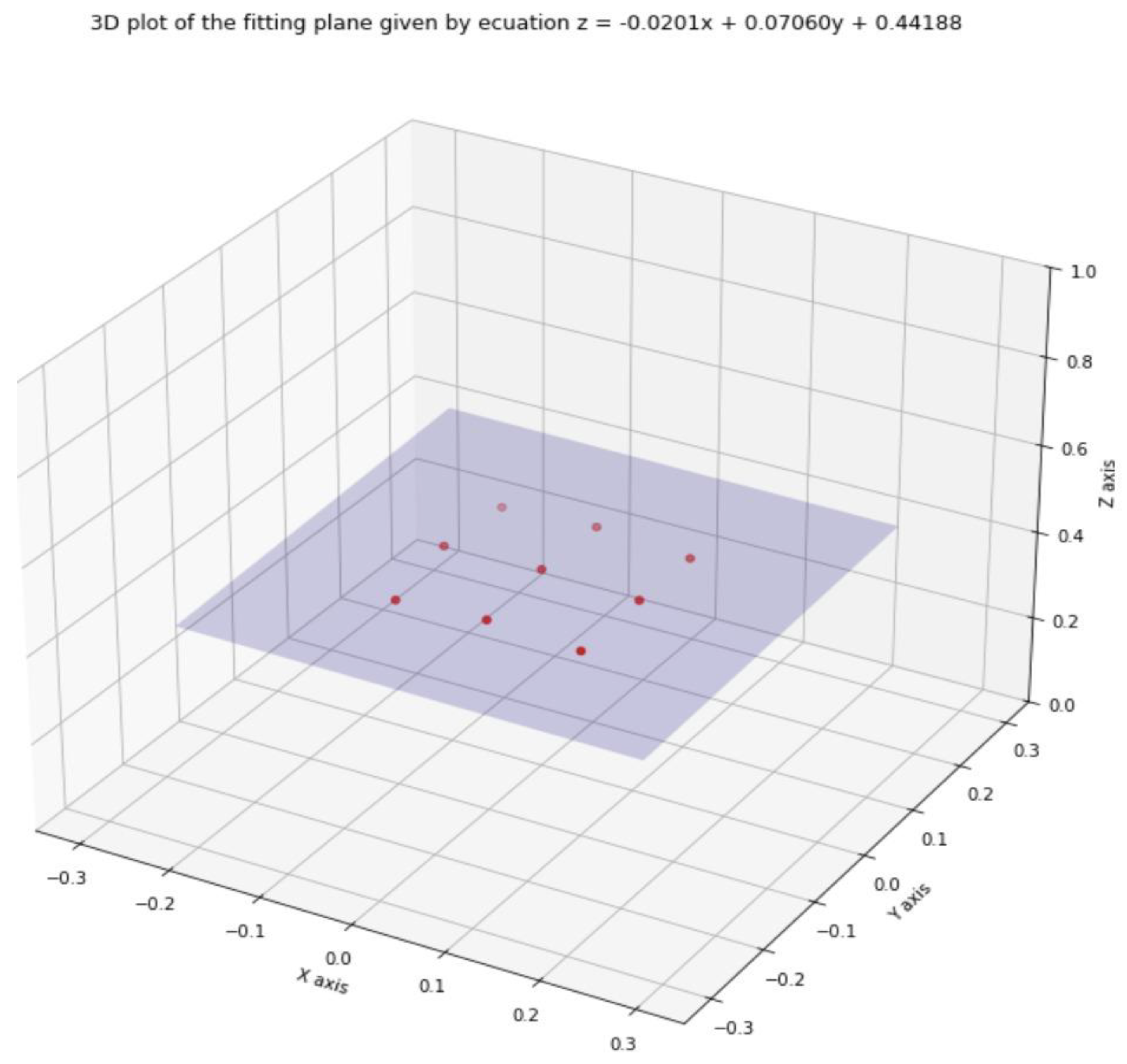
• Points P1 to P9 were all transformed from spherical coordinates into Cartesian coordinates in an XYZ space. In these conditions, the measuring plane is the plane that passes through all nine points. The least square method was used to estimate the coefficients of the fit plane. The fitting plane is defined by the following equation:

  Z = Ax + By + c

  (6)

  where a, b, and c are the solution to the following equation:

  $$⌊\begin{array}{c}a\\ b\\ c\end{array}⌋={\left({⌊\begin{array}{ccc}{x}_1& y_1& 1\\ \dots & \dots & \dots \\ x_n& y_n& 1\end{array}⌋}^T\ast ⌊\begin{array}{ccc}{x}_1& y_1& 1\\ \dots & \dots & \dots \\ x_n& y_n& 1\end{array}⌋\right)}^{-1}\ast {⌊\begin{array}{ccc}{x}_1& y_1& 1\\ \dots & \dots & \dots \\ x_n& y_n& 1\end{array}⌋}^T\ast ⌊\begin{array}{c}{z}_1\\ \dots \\ z_2\end{array}⌋$$

  (7)
• The angles between the fitting plane and the XOY, XOZ, and YOZ planes are calculated. The angle is determined by using the dot product between the vector of the fitting plane (a, b, and −1) and the normal vector of each of the following planes: XOY, XOZ, and YOZ. The angle is given by the following formula:

$$\propto =arccos\left({\displaystyle \frac{a}{\sqrt{a^2+b^2+1}}}\right)$$

(8)

4. Results and Discussion

Since the goal of the study is to develop a camera calibration algorithm that can be used in real-time for robotic vision applications, it is necessary that the procedure is suitable for integration with the camera software. For easier integration with the acquisition software of the 2D/3D camera, all calculation procedures were developed in Python 3.11. In Figure 13, the approach for implementing the proposed camera calibration procedure is shown. This subroutine is important as it represents one of the main contributions of the study. It can be integrated into any robot task that requires camera calibration and it can be accessed whenever necessary. The procedure was further integrated into the camera measurement software for continuous data measurement and validation. All measurements were performed with the same orientation, but at different heights, which were chosen randomly. For all points, there were three measuring sets for three different heights, for four different perimeters for a total of 12 data sets (

Table 2. Raw data (mm).

Data Set	P9			P8			P7
	P6			P5			P4
	P3			P2			P1
H1 20 px	−49	−50	450	0	−40	452	49	−50	447
	−51	−1	463	0	−1	456	51	−1	457
	−51	51	467	0	41	465	51	50	463
H1 30 px	−73	−74	446	0	−74	445	73	−74	444
	−75	−1	456	0	−1	457	74	−1	450
	−77	77	469	0	77	471	77	76	467
H1 40 px	−96	−97	438	0	−98	441	96	−96	435
	−101	−1	458	0	−1	456	99	−1	451
	−102	102	468	0	104	475	103	102	469
H1 50 px	−119	−120	436	0	−120	435	118	−119	432
	−126	−1	458	0	−1	456	125	−1	453
	−129	128	471	0	130	474	128	127	468
H2 20 px	−63	−64	575	0	−60	574	63	−64	572
	−64	1	586	0	1	587	64	−1	583
	−66	65	598	0	61	596	66	65	594
H2 30 px	−94	−95	569	0	−95	568	94	−94	566
	−96	−1	585	0	−1	587	96	−1	578
	−99	98	599	0	99	601	99	98	597
H2 40 px	−123	−124	561	0	−125	564	122	−123	557
	−129	−1	585	0	−1	587	128	−1	580
	−131	131	600	0	133	607	132	131	600
H2 50 px	−151	−152	554	0	−153	555	150	−151	549
	−160	−1	584	0	−1	586	159	−1	577
	−164	164	602	0	166	607	165	164	601
H3 20 px	−66	−67	597	0	−62	596	66	−66	593
	−67	−1	609	0	−1	610	67	−1	606
	−68	68	621	0	61	620	68	67	616
H3 30 px	−98	−99	593	0	−98	590	97	−98	589
	−100	−1	607	0	−1	609	100	−1	602
	−102	102	621	0	102	623	102	101	619
H3 40 px	−128	−129	584	0	−130	586	127	−128	579
	−134	−1	607	0	−1	609	132	−1	601
	−137	136	623	0	138	630	137	136	622
H3 50 px	−158	−159	577	0	−160	579	157	−157	572
	−167	−1	607	0	−1	609	165	−1	600
	−170	170	624	0	172	628	171	170	623

).

For the first approach, the calculated angles for camera inclination are shown in

Table 3. First approach results—law of cosines.

Height	Px	Angle [°]	Error
1	20	81.75414348	2.19%
	30	76.05467223	4.93%
	40	75.04858306	6.19%
	50	72.38921295	9.51%
2	20	74.61077611	6.74%
	30	73.87802451	7.65%
	40	73.32941035	8.34%
	50	70.86462849	11.42%
3	20	74.0954911	7.38%
	30	74.25758952	7.18%
	40	73.72102328	7.85%
	50	71.68477916	10.39%

, together with the error relative to the actual camera rotation angle. Table 3 shows the error levels of the first calibration method when compared to the actual camera angle relative to the measurement plane. As specified above, the measurements were performed at three different height levels denoted in the table as Heights 1, 2, and 3 (in ascending order). The distance between the measurement points and the origin is specified in the second column (ranging from 20 pixels to 50 pixels). The third column illustrates the angle calculated using the law of cosines, while the fourth column specifies the error when compared to the actual camera inclination angle. The error is expressed as a percentage of the angle value. For the second approach, the calculated angles for camera inclination are shown in

Table 4. Second approach results—planar interpolation.

Height	Px	Angle [°]	Error
1	20	79.3466	0.82%
	30	79.2076	0.99%
	40	79.0834	1.15%
	50	80.2278	0.28%
2	20	78.2116	2.24%
	30	79.0063	1.24%
	40	79.1527	1.06%
	50	79.4779	0.65%
3	20	77.9434	2.57%
	30	79.7438	0.32%
	40	79.4375	0.70%
	50	80.1961	0.25%

. The errors relative to the actual camera rotation angle are also displayed as percentages of the angle value.

Considering the experimental procedure described for the first approach, the following algorithm for determining the camera orientation relative to the measuring plane was developed:

• It is worth noting that the lowest error levels were obtained when using the measurement points placed at a 20 pixels distance from the origin.
• The camera acquires the required data for the measured points—that is, the distance to the points as shown in Figure 4 and Figure 5.
• From Figure 5, CO and CA_y are known from the data acquired by the camera. Also, OA_y is known, being the fixed distance imposed between the respective measurement point and the origin O (in this case, corresponding to 20 pixels). These are the input values of the calculation.
• Using the law of cosines, the angle $\propto$ is computed with Equation (5). This represents the camera inclination angle.
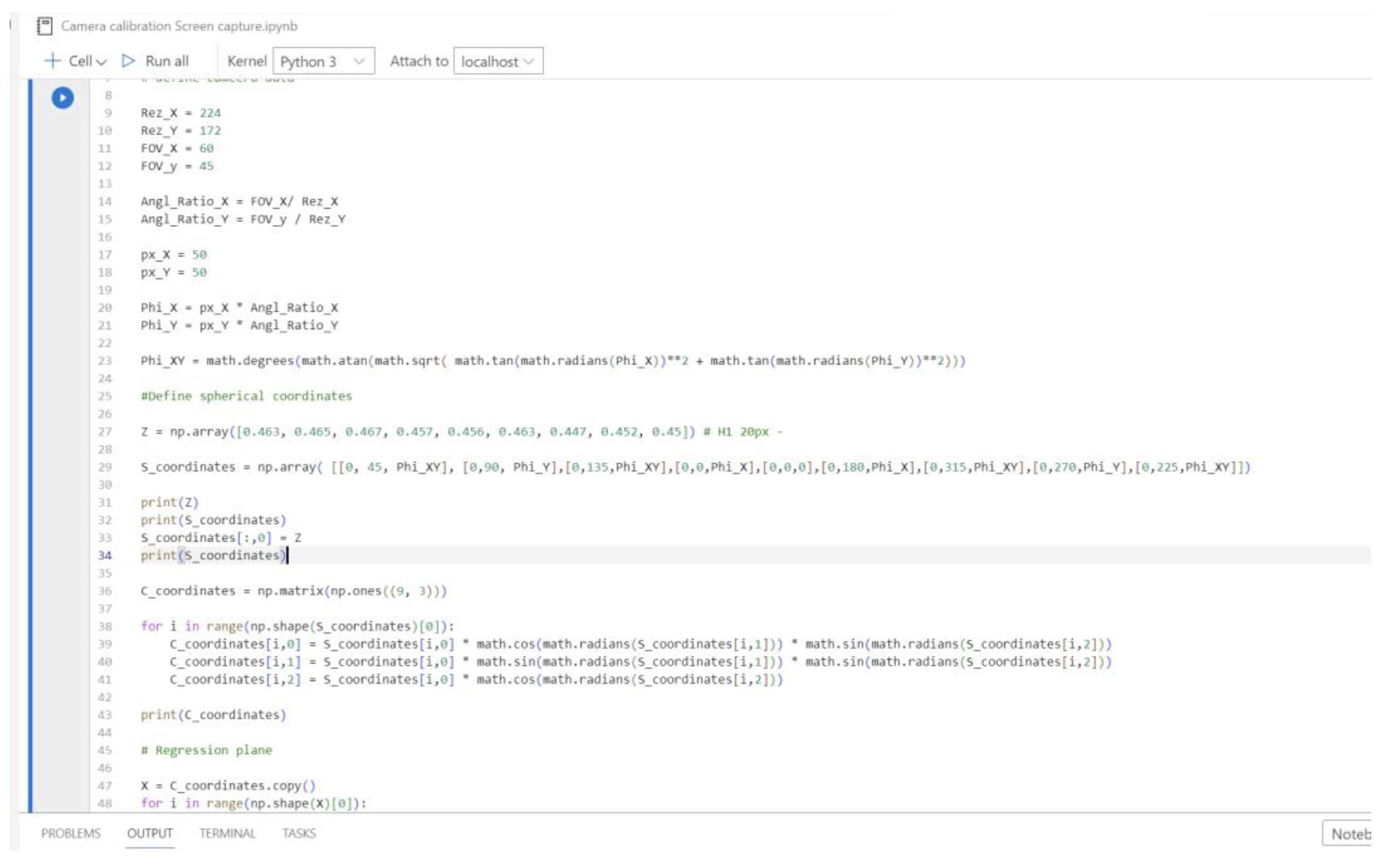
• This algorithm is implemented in the Python program. The subroutine can be applied at any time during a task, by acquiring input data from any planar surface the work objects are placed onto. If a higher level of accuracy for the calculation is required, the camera can be moved within a 20 pixels distance from the measurement plane, since this height showed the lowest error levels—illustrated by Table 3.

For the second approach, planar interpolation (Figure 14), the results are summarized in Table 4, as one can easily observe the error smaller for this method as the plane is calculated based on nine measuring points instead of only three as in the previous method. To further increase the accuracy of this method, for each point an average value could be considered.

The error in column 4 was calculated concerning the imposed angle_real of 80° as in the previous case using Formula (9).

$$Error=\left|{\displaystyle \frac{{Angle}_{experimental}-{Angle}_{real}}{{Angle}_{real}}}\right|·1000 [\%]$$

(9)

Regarding the measurement results and the methods implemented for the calculation of the camera rotation angles, the following aspects should be noted:

• The method using the law of cosines is easier to implement and requires far more computational resources because it uses less data. In the case of the 20 pixels measurement perimeter, for example, the law of cosines approach uses four points, while the planar interpolation approach uses nine measurement points. This observation applies to all measurement perimeters and all measurement heights. Also, the calculation formula for the lay of cosines approach is simpler.
• However, since it uses fewer measurement points, the law of cosines approach is less accurate. The error levels calculated for the first approach, shown in Table 3, are ranging from 2.19% to 11.42%, with an average of 7.48%.
• It is worth noting that the law of cosines itself has some limitations, generating high level of errors for low camera rotation angles. For the most part, the higher level of errors is caused by rounding off the numbers used in calculations and by the uncertainties in the working environment.
• For this study, it was taken into account the fact that the robotic vision feature is used for acquiring data from working environments that are not deterministic. This means that these type of cameras will be used in a setup that has a high number of undetermined variables and deviations. In most cases, these types of applications could include parts with random positions and orientations, measurement surfaces with deviations from the planar shape, fixtures and supports with low accuracy levels (including 3D printed), and so on. The first approach showed that these variations have a higher influence on the results obtained, reflected through a higher error level.
• The method using the planar interpolation was used in order to mitigate the influence of the environmental variables on the camera angle calculation. The procedure is harder to implement and uses more data, thus requiring more computational resources. The calculation is more complex, requiring the employment of the least squares method and conversions between polar coordinates and Cartesian coordinates.
• The accuracy of the second approach proved to be higher. By using more measurement points, the error levels ranged from 0.25% and 2.57%, with an average of 1.02%, as shown in Table 4.
• Due to the specifics of the used mathematical algorithm, the planar interpolation approach can compensate for the errors in measurement data, including those generated by uncertainties in the working environment. This is reflected in a more accurate calculation, as shown above. Furthermore, a larger set of points can be used to flatten the results, thus lowering the overall error.
• The measurements were performed at different heights in order to observe the variations of the error levels at different distances between the camera and the measurement plane. The distance to the measurement points was determined at three different camera heights, chosen randomly.
• For the first approach, the average error level for the first height was 5.7%; for the second height, it was 8.54%, and for the third height, it was 8.2%.
• For the second approach, the average error level for the first height was 0.81%; for the second height, it was 1.3%, and for the third height, it was 0.96%.
• The measuring heights were inserted into the tables in ascending order. It can be observed in both cases that the lowest height yielded the lowest error levels.
• For the first approach, the average error level for the 20 pixels perimeter was 5.44%; for the 30 pixels perimeter, it was 6.59%, for the 40 pixels perimeter, it was 7.46%, and for the 50 pixels perimeter, it was 10.44%.
• For the second approach, the average error level for the 20 pixels perimeter was 1.88%; for the 30 pixels perimeter, it was 0.85%, for the 40 pixels perimeter, it was 0.97%, and for the 50 pixels perimeter, it was 0.39%.
• It can be observed that, as the points are measured on a wider perimeter, in the case of the planar interpolation approach, the error levels decrease. For the law of cosines approach, the error levels increase with the measurement perimeter, as the errors are cumulated due to the nature of the algorithm.
• For both calibration methods, one set of points is enough to determine the position and orientation of the camera relative to the measurement plane at a certain moment. However, as this algorithm was implemented in Python, the results are updated in real-time. Whenever necessary—that is, when the measurement plane changes—the calibration subroutine—the Python program—can be accessed to perform another calibration that will determine the position and orientation of the camera relative to the new measurement plane.
• The errors shown in the analysis (Table 3 and Table 4) are the errors that result when comparing the real camera inclination angle to the calculated angle using the calibration algorithm. It should be noted that these are not object measurement errors. The main purpose of camera calibration is to reduce measurement errors due to image deformations induced by perspective. While it is true that a more precise calibration yields more precise results when measuring objects, any level of calibration would ultimately reduce measurement errors by some amount. Thus, it must be taken into account that, while in some cases presented above the calibration errors may reach or exceed 10%, the measurement errors induced by these offsets would be much lower. The overall assembly accuracy is determined by the 2D camera used; the calibration process itself just improves the measuring process.

5. Conclusions

The presented study was focused on robotic vision systems, with the main subject being camera calibration for robotic applications. The main goal of the research was to develop a method for calibrating the camera with respect to the measurement plane—the plane in which the detected objects are placed. The calibration method was developed using two approaches, the first based on the law of cosines and the second based on plane interpolation. The calculations regarding camera inclination were checked in both cases using the experimental setup. Based on the obtained results, the following conclusions were drawn:

• By using two approaches for camera calibration, with different calculation methods, the results could be discussed through comparative analysis. This allowed to highlight the advantages and disadvantages of each method. While the law of cosines approach is simpler and easier to implement, without further refining, the high error levels make it unsuitable to be integrated in robotic vision applications.
• The average error of around 1% for the plane interpolation approach is acceptable for most robotic applications. At a wider angle, a 70° angle, for example, the error is around 0.7°.
• The planar interpolation approach has the advantage of an increased level of precision for wider spacing between the measurement points. Also, while there is a decrease in precision for greater camera heights, the error levels still remain around 1%.
• The described method does not require any calibration sheet or other dedicated materials, which makes it suitable for almost any workspace configuration. Using this procedure, the calibration can be performed in any position during operation, thus lowering the time required.
• Even though this calibration method sometimes has a lower accuracy, it is more suitable for some unstructured applications like those in which the position of the robot changes over time (i.e., robots mounted on mobile platforms, unstructured pick and place assembly operations), where other calibration methods, like the one implying a calibration pattern, are difficult to implement. This method could be implemented in real-time during robot operation, while other calibration methods are usually performed before robot operation.
• The Python code is easy to develop for the proposed calibration algorithm and it can be integrated with most acquisition software.
• By integrating the Python code with the acquisition software, the input data can be fed to the system in real-time, which means that the calibration can be performed while the application is running. Thus, the data acquisition software can adapt immediately to any changes in the working environment, and periodical calibration cycles are no longer necessary.
• The calibration method described in this study holds significant potential to enhance results in industrial robotic applications, such as pick and place and assembly, and in other fields employing vision systems.

The presented research developed a framework for camera calibration that has certain advantages, as highlighted above. Besides these considerations, it is also worth noting that the proposed method can be used to improve productivity for applications that require camera calibration. Since no separate calibration procedure is required and the developed Python subroutine can be used at any moment, the calibration can be performed without interrupting the robot program, which reduces cycle times. Also, these aspects make the procedure more convenient when compared to other approaches, even more so when taking into account that no printed calibration sheet is required. This implies that the need for a dedicated calibration area and correct calibration planning within the robot task is eliminated, which also frees up the robot workspace. Based on this framework, future studies can refine and improve the described methods, considering the specifics of various applications.

Another advantage of the proposed method is linked to the specifics of unstructured applications. Without using a vision system, such applications must resort to other solutions for solving various uncertainties, such as using a gravitational part aligning support. These solutions introduce an additional operation to the task, affecting cycle times and productivity. This in especially critical in high-speed applications. The solution proposed in this study removes the need for such additional operations, thus reducing cycle times. Also, by embedding the calibration procedure into the assembly task (without performing a separate calibration operation), the productivity of the entire application is improved.

For a typical camera calibration procedure, because a printed template is required, the camera must be positioned above the template in a dedicated area. This implies additional movement of the robot arm. After the camera is positioned, the calibration generally takes around 2 s, because camera focalization must also be performed. After the calibration, the robot must again reposition itself in the application workspace to resume the assembly task. The duration of the robot movements is highly dependent on the application. By using the proposed calibration method, not only is the need for additional robot movements eliminated, but, also, the calibration together with the measuring process takes around 1 s (as resulted from the experimental validation). The calibration itself takes less than 0.3 s due to the embedded calibration procedure and lightweight program used to implement the calculations.

That being said, the proposed method is especially useful in situations in assembly operations that must meet tight productivity criteria, given that the main advantage provided is linked to the reduction of cycle times, as shown above. Thus, the most adequate scenario would be the case of high-speed assembly tasks that include a large number of parts and have an unstructured environment, such as electronics assembly. Since the calibration is required before each measurement, assembling a large number of parts would benefit mostly from the proposed method since the calibration would be done during the assembly operation itself.

Future research will integrate the developed mathematical model into a high-speed robot assembly system. To achieve that, the proposed model needs to be integrated into the robotic software.

References

- Arents, J.; Greitans, M. Smart Industrial Robot Control Trends, Challenges and Opportunities within Manufacturing. Appl. Sci. 2022, 12, 937. [Google Scholar] [CrossRef]
- Javaid, M.; Haleem, A.; Singh, R.P.; Suman, R. Substantial capabilities of robotics in enhancing industry 4.0 implementation. Cogn. Robot. 2021, 1, 58–75. [Google Scholar] [CrossRef]
- Javaid, M.; Haleem, A.; Singh, R.P.; Rav, S.; Suman, R. Significance of sensors for industry 4.0: Roles, capabilities, and applications. Sens. Int. 2021, 2, 100110. [Google Scholar] [CrossRef]
- Evjemo, L.D.; Gjerstad, T.; Grøtli, E.I.; Sziebig, G. Trends in Smart Manufacturing: Role of Humans and Industrial Robots in Smart Factories. Curr. Robot. Rep. 2020, 1, 35–41. [Google Scholar] [CrossRef]
- Jia, F.; Ma, Y.; Ahmad, R. Review of current vision-based robotic machine-tending applications. Int. J. Adv. Manuf. Technol. 2024, 131, 1039–1057. [Google Scholar] [CrossRef]
- Khang, A.; Misra, A.; Abdullayev, V.; Litvinova, E. Machine Vision and Industrial Robotics in Manufacturing: Approaches, Technologies, and Applications; CRC Press: Boca Raton, FL, USA, 2024. [Google Scholar] [CrossRef]
- Niu, L.; Saarinen, M.; Tuokko, R.; Mattila, J. Integration of Multi-Camera Vision System for Automatic Robotic Assembly. Procedia Manuf. 2019, 37, 380–384. [Google Scholar] [CrossRef]
- Song, R.; Li, F.; Fu, T.; Zhao, J. A Robotic Automatic Assembly System Based on Vision. Appl. Sci. 2020, 10, 1157. [Google Scholar] [CrossRef]
- Karnik, N.; Bora, U.; Bhadri, K.; Kadambi, P.; Dhatrak, P. A comprehensive study on current and future trends towards the characteristics and enablers of industry 4.0. J. Ind. Inf. Integr. 2022, 27, 100294. [Google Scholar] [CrossRef]
- Goel, R.; Gupta, P. Robotics and Industry 4.0. In A Roadmap to Industry 4.0: Smart Production, Sharp Business and Sustainable Development; Advances in Science, Technology & Innovation; Springer: Cham, Switzerland, 2020. [Google Scholar] [CrossRef]
- Grau, A.; Indri, M.; Lo Bello, L.; Sauter, T. Robots in Industry: The Past, Present, and Future of a Growing Collaboration with Humans. IEEE Ind. Electron. Mag. 2021, 15, 50–61. [Google Scholar] [CrossRef]
- Grau, A.; Indri, M.; Lo Bello, L.; Sauter, T. Industrial robotics in factory automation: From the early stage to the Internet of Things. In Proceedings of the IECON 2017—43rd Annual Conference of the IEEE Industrial Electronics Society 2017, Beijing, China, 29 October–1 November 2017; pp. 6159–6164. [Google Scholar] [CrossRef]
- Avalle, G.; De Pace, F.; Fornaro, C.; Manuri, F.; Sanna, A. An augmented reality system to support fault visualization in industrial robotic tasks. IEEE Access 2019, 7, 132343–132359. [Google Scholar] [CrossRef]
- Matheson, E.; Minto, R.; Zampieri, E.G.G.; Faccio, M.; Rosati, G. Human–Robot Collaboration in Manufacturing Applications: A Review. Robotics 2019, 8, 100. [Google Scholar] [CrossRef]
- Wang, Z.; Fan, J.; Jing, F.; Deng, S.; Zheng, M.; Tan, M. An Efficient Calibration Method of Line Structured Light Vision Sensor in Robotic Eye-in-Hand System. IEEE Sens. J. 2020, 20, 6200–6208. [Google Scholar] [CrossRef]
- Enebuse, I.; Foo, M.; Ibrahim, B.S.K.K.; Ahmed, H.; Supmak, F.; Eyobu, O.S. A Comparative Review of Hand-Eye Calibration Techniques for Vision Guided Robots. IEEE Access 2021, 9, 113143–113155. [Google Scholar] [CrossRef]
- Qi, W.; Li, F.; Zhenzhong, L. Review on camera calibration. In Proceedings of the 2010 Chinese Control and Decision Conference, Xuzhou, China, 26–28 May 2010; pp. 3354–3358. [Google Scholar] [CrossRef]
- Gong, X.; Lv, Y.; Xu, X.; Jiang, Z.; Sun, Z. High-precision calibration of omnidirectional camera using an iterative method. IEEE Access 2019, 7, 152179–152186. [Google Scholar] [CrossRef]
- Lee, T.E.; Tremblay, J.; To, T.; Cheng, J.; Mosier, T.; Kroemer, O.; Fox, D.; Birchfield, S. Camera-to-Robot Pose Estimation from a Single Image. In Proceedings of the 2020 IEEE International Conference on Robotics and Automation (ICRA), Paris, France, 31 May–31 August 2020; pp. 9426–9432. [Google Scholar] [CrossRef]
- Wang, X.; Chen, H.; Li, Y.; Huang, H. Online Extrinsic Parameter Calibration for Robotic Camera–Encoder System. IEEE Trans. Ind. Inform. 2019, 15, 4646–4655. [Google Scholar] [CrossRef]
- Zhang, Y.-J. 3-D Computer Vision: Principles, Algorithms and Applications, 1st ed.; Springer: Singapore, 2023. [Google Scholar] [CrossRef]
- Chang, W.-C.; Wu, C.-H. Eye-in-hand vision-based robotic bin-picking with active laser projection. Int. J. Adv. Manuf. Technol. 2016, 85, 2873–2885. [Google Scholar] [CrossRef]
- Roberti, A.; Piccinelli, N.; Meli, D.; Muradore, R.; Fiorini, P. Improving Rigid 3-D Calibration for Robotic Surgery. IEEE Trans. Med. Robot. Bionics 2020, 2, 69–573. [Google Scholar] [CrossRef]
- Ramírez-Hernández, L.R.; Rodríguez-Quiñonez, J.C.; Castro-Toscano, M.J.; Hernandez-Balbuena, D.; Flores-Fuentes, W.; Rascon-Carmona, R.; Lindner, L.; Sergiyenko, O. Improve three-dimensional point localization accuracy in stereo vision systems using a novel camera calibration method. Int. J. Adv. Robot. Syst. 2020, 17, 1729881419896717. [Google Scholar] [CrossRef]
- Zhang, Z. A flexible new technique for camera calibration. IEEE Trans. Pattern Anal. Mach. Intell. 2000, 22, 1330–1334. [Google Scholar] [CrossRef]
- Jiang, T.; Cui, H.; Cheng, X. A calibration strategy for vision-guided robot assembly system of large cabin. Measurement 2020, 163, 107991. [Google Scholar] [CrossRef]
- Ma, X.; Zhu, P.; Li, X.; Zheng, X.; Zhou, J.; Wang, X.; Wai, K.; Au, S. A Minimal Set of Parameters-Based Depth-Dependent Distortion Model and Its Calibration Method for Stereo Vision Systems. IEEE Trans. Instrum. Meas. 2024, 73, 7004111. [Google Scholar] [CrossRef]
- Yi, H.; Song, K.; Song, X. Watermelon Detection and Localization Technology Based on GTR-Net and Binocular Vision. IEEE Sens. J. 2024, 24, 19873–19881. [Google Scholar] [CrossRef]
- Guo, R.; Cui, H.; Deng, Y.; Yang, R.; Jiang, T. An Accurate Volumetric Error Modeling Method for a Stereo Vision System Based on Error Decoupling. IEEE Trans. Instrum. Meas. 2024, 73, 5020112. [Google Scholar] [CrossRef]
- Gunady, I.E.; Ding, L.; Singh, D.; Alfaro, B.; Hultmark, M.; Smiths, A.J. A non-intrusive volumetric camera calibration system. Meas. Sci. Technol. 2024, 35, 105901. [Google Scholar] [CrossRef]
- Peng, G.; Ren, Z.; Gao, Q.; Fan, Z. Reprojection Error Analysis and Algorithm Optimization of Hand–Eye Calibration for Manipulator System. Sensors 2024, 24, 113. [Google Scholar] [CrossRef]
- Zeng, R.; Zhao, Y.; Chen, Y. Camera calibration using the dual double-contact property of circles. J. Opt. Soc. Am. A 2023, 40, 2084–2095. [Google Scholar] [CrossRef]
- Chen, L.; Zhong, G.; Wan, Z.; Han, Z.; Liang, X.; Pan, H. A novel binocular vision-robot hand-eye calibration method using dual nonlinear optimization and sample screening. Mechatronics 2023, 96, 103083. [Google Scholar] [CrossRef]