

Per-Instance Algorithm Configuration in Homogeneous Instance Spaces: A Use Case in Reconfigurable Assembly Systems
 , , , and
Abstract
1. Introduction
2. Related Work
- (i)
- Once again, they are related to generalization, as it is possible to find unique configurations outside of the portfolio with better performance than the best “average” configurator of the class for individual instances within the class,
- (ii)
- the expensive Exploration of the configuration space, since each new configuration explored needs to be evaluated against all (or a representative set of) the available problem instances. This is nonetheless a very expensive approach that limits the set of configurations that can eventually be explored (although some arguments in favor of this approach appear in the literature as a countermeasure to over-tuning [10,16]).
- (iii)
- Consequently, it becomes rather expensive to augment the portfolio (if, e.g., a new instance class or a new configuration with possible performance gains is identified), since adding a new configuration would require its evaluation in a large number of instances.
3. Methods
3.1. Case-Based Reasoning Method for PIAC
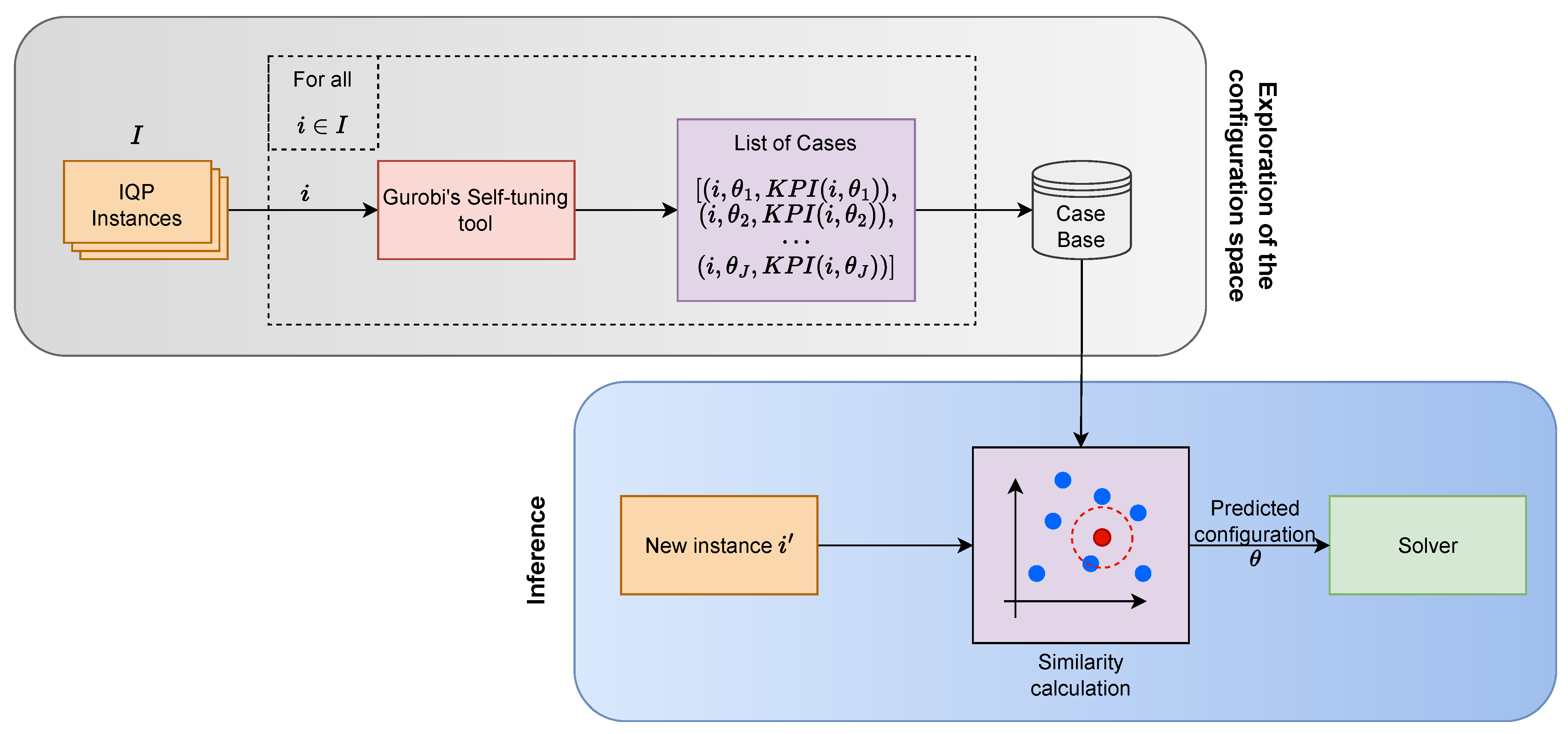
3.1.1. Exploration of the Configuration Space
- Adaptive capping, for instance, is one of the features reported by Gurobi [21] (it is also easy to identify the adaptive capping feature in action when tuning is focused on algorithm runtime). It is a common feature proved to increase search performance and can be observed in many state-of-the-art configurators such as ParamILS [30], GGA [29], and Irace [41].
- The summary of the best configurations found follows a Pareto frontier [21] that focuses on configurations with fewer perturbations over the base/default settings.
- It performs replications with different random seeds to obtain more robust performance estimates [21].
- It allows for a secondary performance measure to guide the configuration search for instances that do not solve to optimality [21]; in such cases, solution quality becomes more relevant than the runtime, and thus available options include the minimization of the optimality gap, the best solution found (that with the best objective value), or the best objective bound.
- It allows for distributed parallel tuning [21], e.g., to distribute the tuning task over different CPUs in a computer cluster.
- The definition of a minimum acceptable performance target [21] so that tuning can stop once a minimum predefined performance is reached.
- It combines expert knowledge by means of certain “rules of thumb” in order to guide the search in combination with a random search [42].
- TuneResults (this tuning tool setting defines the number of configurations that yield an improvement over the default Gurobi settings that are eventually reported by the tool, which we will set to 10);
- TuneTrials (this tuning tool setting defines the number of replications that are run for each configuration on each instance, which we will set to 3);
- To investigate the performance of the PIAC method in relation to the budget allocated for the exploration of the configuration space, we will change the value of the setting TuneTimeLimit (this tuning tool setting defines the CPU time allocated to the tuning tool) accordingly (see Section 5.1).
3.1.2. Training and Inference
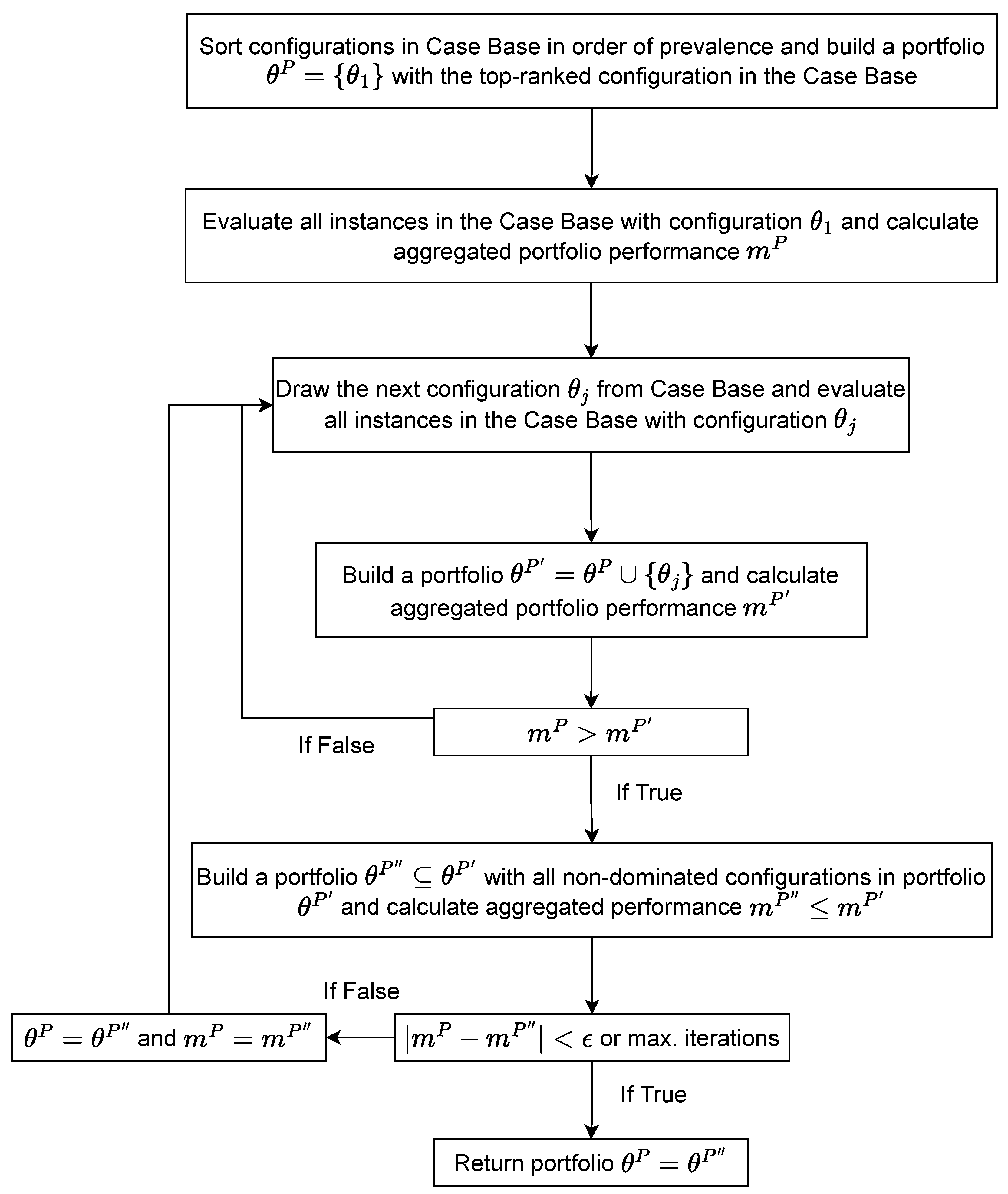
3.2. Portfolio Method for PIAC: Hydra
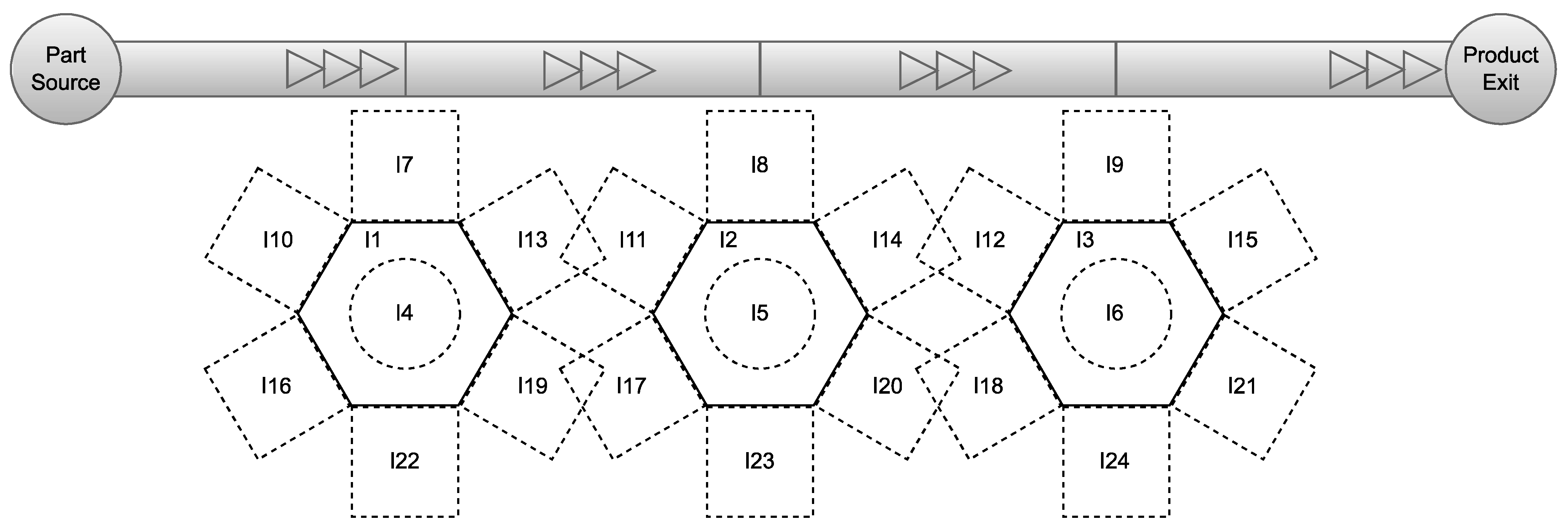
4. Use Case Definition
5. Experimental Methodology
5.1. Sampling Procedure
5.2. Instance Features
5.3. Evaluation Methodology
6. Experiments and Discussion
6.1. Evaluation of the CBR Method for PIAC


| Metric | Avg. PAR-10 Reduction | Avg. CPU Time Reduction | Avg. Reduction in the Number of Timed-Out Replications |
|---|---|---|---|
| From 100 to 800 instances @ Case Base 1 | [−2.34, 3.34] | [−1.41, 0.84] | [−2.49, 3.70] |
| From 100 to 800 instances @ Case Base 2 | [−0.57, 5.02] | [−0.78, 1.40] | [−0.57, 5.55] |
| From 100 to 800 instances @ Case Base 3 | [−1.53, 3.89] | [−1.08, 1.09] | [−1.62, 4.30] |
| From Case Base 1 to Case Base 2 a | [5.88, 7.07] | [1.50, 1.94] | [6.49, 7.79] |
| From Case Base 1 to Case Base 3 a | [7.70, 9.27] | [2.16, 2.63] b | [8.49, 10.21] |
| From Case Base 2 to Case Base 3 a | [1.54, 2.48] | [0.41, 0.72] | [1.69, 2.74] |

6.2. Evaluation of Hydra: A Portfolio Method for PIAC

| Metric | Avg. PAR-10 Reduction |
|---|---|
| From 100 to 800 instances @ Case Base 1 | [−1.78, 3.74] b |
| From 100 to 800 instances @ Case Base 2 | [−9.33, −1.75] |
| From 100 to 800 instances @ Case Base 3 | [−6.27, 2.86] |
| From Case Base 1 to Case Base 2 a | [−0.38, 3.07] b |
| From Case Base 1 to Case Base 3 a | [−6.63, −3.93] b |
| From Case Base 2 to Case Base 3 a | [−7.80, −4.70] b |

6.3. Discussion
7. Conclusions and Future Work
Author Contributions
Funding
Institutional Review Board Statement
Informed Consent Statement
Data Availability Statement
Conflicts of Interest
References
- Koren, Y.; Gu, X.; Guo, W. Reconfigurable manufacturing systems: Principles, design, and future trends. Front. Mech. Eng. 2018, 13, 121–136. [Google Scholar] [CrossRef]
- Dou, J.; Li, J.; Xia, D.; Zhao, X. A multi-objective particle swarm optimisation for integrated configuration design and scheduling in reconfigurable manufacturing system. Int. J. Prod. Res. 2021, 59, 3975–3995. [Google Scholar] [CrossRef]
- Bensmaine, A.; Dahane, M.; Benyoucef, L. A new heuristic for integrated process planning and scheduling in reconfigurable manufacturing systems. Int. J. Prod. Res. 2014, 52, 3583–3594. [Google Scholar] [CrossRef]
- Stützle, T.; López-Ibáñez, M. Automated design of metaheuristic algorithms. In Handbook of Metaheuristics; Springer: Cham, Switzerland, 2019; pp. 541–579. [Google Scholar]
- Hutter, F.; Babic, D.; Hoos, H.H.; Hu, A.J. Boosting verification by automatic tuning of decision procedures. In Proceedings of the Formal Methods in Computer Aided Design (FMCAD’07), Austin, TX, USA, 11–14 November 2007; IEEE: Piscataway, NJ, USA, 2007; pp. 27–34. [Google Scholar]
- Schede, E.; Brandt, J.; Tornede, A.; Wever, M.; Bengs, V.; Hüllermeier, E.; Tierney, K. A survey of methods for automated algorithm configuration. J. Artif. Intell. Res. 2022, 75, 425–487. [Google Scholar] [CrossRef]
- Ortiz-Bayliss, J.C.; Amaya, I.; Cruz-Duarte, J.M.; Gutierrez-Rodriguez, A.E.; Conant-Pablos, S.E.; Terashima-Marín, H. A general framework based on machine learning for algorithm selection in constraint satisfaction problems. Appl. Sci. 2021, 11, 2749. [Google Scholar] [CrossRef]
- Kerschke, P.; Hoos, H.H.; Neumann, F.; Trautmann, H. Automated algorithm selection: Survey and perspectives. Evol. Comput. 2019, 27, 3–45. [Google Scholar] [CrossRef] [PubMed]
- Rice, J.R. The algorithm selection problem. In Advances in Computers; Elsevier: Amsterdam, The Netherlands, 1976; Volume 15, pp. 65–118. [Google Scholar]
- Kadioglu, S.; Malitsky, Y.; Sellmann, M.; Tierney, K. ISAC—Instance-specific algorithm configuration. In Proceedings of the ECAI 2010—19th European Conference on Artificial Intelligence, Lisbon, Portugal, 16–20 August 2010; IOS Press: Amsterdam, The Netherlands, 2010; pp. 751–756. [Google Scholar]
- Xu, L.; Hoos, H.; Leyton-Brown, K. Hydra: Automatically configuring algorithms for portfolio-based selection. In Proceedings of the AAAI Conference on Artificial Intelligence, Atlanta, GA, USA, 11–15 July 2010; Volume 24, pp. 210–216. [Google Scholar]
- Xu, L.; Hutter, F.; Hoos, H.H.; Leyton-Brown, K. Hydra-MIP: Automated algorithm configuration and selection for mixed integer programming. In Proceedings of the RCRA Workshop on Experimental Evaluation of Algorithms for Solving Problems with Combinatorial Explosion at the International Joint Conference on Artificial Intelligence (IJCAI), Barcelona, Spain, 17–18 July 2011; pp. 16–30. [Google Scholar]
- Bhosale, K.C.; Pawar, P.J. Production planning and scheduling problem of continuous parallel lines with demand uncertainty and different production capacities. J. Comput. Des. Eng. 2020, 7, 761–774. [Google Scholar] [CrossRef]
- Toth, P.; Vigo, D. An overview of vehicle routing problems. In The Vehicle Routing Problem; SIAM: Philadelphia, PA, USA, 2002; pp. 1–26. [Google Scholar]
- Mantovani, S.; Morganti, G.; Umang, N.; Crainic, T.G.; Frejinger, E.; Larsen, E. The load planning problem for double-stack intermodal trains. Eur. J. Oper. Res. 2018, 267, 107–119. [Google Scholar] [CrossRef]
- Eggensperger, K.; Lindauer, M.; Hutter, F. Pitfalls and best practices in algorithm configuration. J. Artif. Intell. Res. 2019, 64, 861–893. [Google Scholar] [CrossRef]
- Belkhir, N.; Dréo, J.; Savéant, P.; Schoenauer, M. Per instance algorithm configuration of CMA-ES with limited budget. In Proceedings of the Genetic and Evolutionary Computation Conference, Berlin, Germany, 15–19 July 2017; pp. 681–688. [Google Scholar]
- Hosny, A.; Reda, S. Automatic MILP solver configuration by learning problem similarities. In Annals of Operations Research; Springer: Berlin/Heidelberg, Germany, 2023; pp. 1–28. [Google Scholar]
- Uzunosmanoglu, M.; Raa, B.; Limère, V.; De Cock, A.; Singh, Y.; Lopez, A.J.; Gautama, S.; Cottyn, J. Aggregate planning for multi-product assembly lines with reconfigurable cells. In Proceedings of the IFIP International Conference on Advances in Production Management Systems, Nantes, France, 5–9 September 2021; Springer: Berlin/Heidelberg, Germany, 2021; pp. 525–534. [Google Scholar]
- Guzman Vargas, D.; Gautama, S.; Uzunosmanoglu, M.; Raa, B.; Limère, V. Per-Instance Algorithm Configuration for Production Planning in a Reconfigurable Assembly System. In Proceedings of the 2024 IEEE 22nd Mediterranean Electrotechnical Conference (MELECON), Porto, Portugal, 25–27 June 2024. [Google Scholar]
- Gurobi Optimization LLC. Gurobi Optimizer Reference Manual; Gurobi Optimization LLC: Beaverton, OR, USA, 2023. [Google Scholar]
- Eryoldaş, Y.; Durmuşoglu, A. A literature survey on offline automatic algorithm configuration. Appl. Sci. 2022, 12, 6316. [Google Scholar] [CrossRef]
- Hoos, H.H. Automated algorithm configuration and parameter tuning. In Autonomous Search; Springer: Berlin/Heidelberg, Germany, 2012; pp. 37–71. [Google Scholar]
- Díaz de León-Hicks, E.; Conant-Pablos, S.E.; Ortiz-Bayliss, J.C.; Terashima-Marín, H. Addressing the Algorithm Selection Problem through an Attention-Based Meta-Learner Approach. Appl. Sci. 2023, 13, 4601. [Google Scholar] [CrossRef]
- Hutter, F.; Xu, L.; Hoos, H.H.; Leyton-Brown, K. Algorithm runtime prediction: Methods & evaluation. Artif. Intell. 2014, 206, 79–111. [Google Scholar]
- O’Mahony, E.; Hebrard, E.; Holland, A.; Nugent, C.; O’Sullivan, B. Using case-based reasoning in an algorithm portfolio for constraint solving. In Proceedings of the Irish Conference on Artificial Intelligence and Cognitive Science, Cork, Ireland, 27 August 2008; pp. 210–216. [Google Scholar]
- Ladosz, P.; Banjo, O.; De Guido, S.; Zalasiewicz, M. A genetic algorithm optimiser for dynamic product routing in agile manufacturing environment. In Proceedings of the 2018 IEEE 16th International Conference on Industrial Informatics (INDIN), Porto, Portugal, 18–20 July 2018; IEEE: Piscataway, NJ, USA, 2018; pp. 1079–1084. [Google Scholar]
- Hutter, F.; Hoos, H.H.; Leyton-Brown, K. Sequential model-based optimization for general algorithm configuration. In Proceedings of the Learning and Intelligent Optimization: 5th International Conference, LION 5, Rome, Italy, 17–21 January 2011; Selected Papers 5. Springer: Berlin/Heidelberg, Germany, 2011; pp. 507–523. [Google Scholar]
- Ansótegui, C.; Sellmann, M.; Tierney, K. A gender-based genetic algorithm for the automatic configuration of algorithms. In Proceedings of the International Conference on Principles and Practice of Constraint Programming, Lisbon, Portugal, 20–24 September 2009; Springer: Berlin/Heidelberg, Germany, 2009; pp. 142–157. [Google Scholar]
- Hutter, F.; Hoos, H.H.; Leyton-Brown, K.; Stützle, T. ParamILS: An automatic algorithm configuration framework. J. Artif. Intell. Res. 2009, 36, 267–306. [Google Scholar] [CrossRef]
- Anand, R.; Aggarwal, D.; Kumar, V. A comparative analysis of optimization solvers. J. Stat. Manag. Syst. 2017, 20, 623–635. [Google Scholar] [CrossRef]
- Khoshniyat, F.; Törnquist Krasemann, J. Analysis of strengths and weaknesses of a MILP model for revising railway traffic timetables. In Proceedings of the 17th Workshop on Algorithmic Approaches for Transportation Modelling, Optimization, and Systems (ATMOS 2017), Vienna, Austria, 4–8 September 2017; Schloss-Dagstuhl-Leibniz Zentrum für Informatik: Wadern, Germany, 2017. [Google Scholar]
- Bunel, R.; Turkaslan, I.; Torr, P.H.; Kohli, P.; Kumar, M.P. Piecewise Linear Neural Networks Verification: A Comparative Study. In Proceedings of the ICLR 2018 Conference, Vancouver, BC, Canada, 30 April–3 May 2018. [Google Scholar]
- Nau, C.; Sankaran, P.; McConky, K. Comparison of Parameter Tuning Strategies for Team Orienteering Problem (TOP) Solved with Gurobi. In Proceedings of the IISE Annual Conference & Expo 2022, Washington, DC, USA, 21–24 May 2022; pp. 1–6. [Google Scholar]
- Böther, M.; Kißig, O.; Taraz, M.; Cohen, S.; Seidel, K.; Friedrich, T. What’s Wrong with Deep Learning in Tree Search for Combinatorial Optimization. arXiv 2022, arXiv:2201.10494. [Google Scholar]
- Wuyckens, S.; Zhao, L.; Saint-Guillain, M.; Janssens, G.; Sterpin, E.; Souris, K.; Ding, X.; Lee, J.A. Bi-criteria Pareto optimization to balance irradiation time and dosimetric objectives in proton arc therapy. Phys. Med. Biol. 2022, 67, 245017. [Google Scholar] [CrossRef] [PubMed]
- Vlk, M.; Novak, A.; Hanzalek, Z. Makespan Minimization with Sequence-dependent Non-overlapping Setups. In Proceedings of the ICORES 2019, Prague, Czech Republic, 19–21 February 2019; pp. 91–101. [Google Scholar]
- Barth, L.; Hagenmeyer, V.; Ludwig, N.; Wagner, D. How much demand side flexibility do we need? Analyzing where to exploit flexibility in industrial processes. In Proceedings of the Ninth International Conference on Future Energy Systems, Karlsruhe, Germany, 12–15 June 2018; pp. 43–62. [Google Scholar]
- Vlk, M.; Novak, A.; Hanzalek, Z.; Malapert, A. Non-overlapping sequence-dependent setup scheduling with dedicated tasks. In Proceedings of the International Conference on Operations Research and Enterprise Systems, Prague, Czech Republic, 19–21 February 2019; Springer: Berlin/Heidelberg, Germany, 2019; pp. 23–46. [Google Scholar]
- Kemminer, R.; Lange, J.; Kempkes, J.P.; Tierney, K.; Weiß, D. Configuring Mixed-Integer Programming Solvers for Large-Scale Instances. In Proceedings of the Operations Research Forum, Munich, Germany, 14 June 2024; Springer: Berlin/Heidelberg, Germany, 2024; Volume 5, pp. 1–14. [Google Scholar]
- López-Ibáñez, M.; Dubois-Lacoste, J.; Cáceres, L.P.; Birattari, M.; Stützle, T. The irace package: Iterated racing for automatic algorithm configuration. Oper. Res. Perspect. 2016, 3, 43–58. [Google Scholar] [CrossRef]
- Gurobi Optimization LLC. Using the Automatic Parameter Tuning Tool. 2013. Available online: https://www.gurobi.com/events/using-the-automatic-parameter-tuning-tool (accessed on 8 March 2024).
- Steffy, D. What Is Parameter Tuning? 2023. Available online: https://support.gurobi.com/hc/en-us/articles/19998635021713-What-is-parameter-tuning- (accessed on 8 March 2024).
- Ting, K.M. An instance-weighting method to induce cost-sensitive trees. IEEE Trans. Knowl. Data Eng. 2002, 14, 659–665. [Google Scholar] [CrossRef]
- Lin, C.D.; Tang, B. Latin hypercubes and space-filling designs. In Handbook of Design and Analysis of Experiments; CRC Press: Boca Raton, FL, USA, 2015; pp. 593–625. [Google Scholar]
- Lilliefors, H.W. On the Kolmogorov-Smirnov test for normality with mean and variance unknown. J. Am. Stat. Assoc. 1967, 62, 399–402. [Google Scholar] [CrossRef]
- Shapiro, S.S.; Wilk, M.B. An analysis of variance test for normality (complete samples). Biometrika 1965, 52, 591–611. [Google Scholar] [CrossRef]
- Stephens, M.A. EDF statistics for goodness of fit and some comparisons. J. Am. Stat. Assoc. 1974, 69, 730–737. [Google Scholar] [CrossRef]
- Box, G.E.; Cox, D.R. An analysis of transformations. J. R. Stat. Soc. Ser. B Stat. Methodol. 1964, 26, 211–243. [Google Scholar] [CrossRef]
- Johnson, R.W. An introduction to the bootstrap. Teach. Stat. 2001, 23, 49–54. [Google Scholar] [CrossRef]


| Case Base Type | Case Base 1 | Case Base 2 | Case Base 3 |
|---|---|---|---|
| Tuning budget per problem instance (s) | 200 | 400 | 600 |
| Total number of instances | 1000 | 1000 | 1000 |
| Total number of (instance, configuration) pairs | 4753 | 3344 | 3305 |
| Total number of unique configurations | 720 | 1437 | 1724 |
| CPU time in seconds a (default; best configuration) | (2.57; 2.19) | (2.57; 2.11) | (2.57; 2.05) |
| PAR-10 in seconds a (default; best configuration) | (20.82; 12.02) | (20.82; 11.10) | (20.82; 10.06) |
| Number of capped replications a (default; best configuration) | (2.03; 1.09) | (2.03; 1.00) | (2.03; 0.89) |
| Number of instances with no capped replications (default; best configuration) | (171; 508) | (171; 594) | (171; 650) |
| Metric | Case Base Size | Case Base Type | Method | ||||
|---|---|---|---|---|---|---|---|
| 100 | 200 | 400 | 600 | 800 | Case Base 1 | CBR method | |
| Avg. PAR-10 reduction (s) | [1.16, 2.34] | [1.34, 2.43] | [1.26, 2.11] | [1.39, 2.16] | [1.43, 2.29] | ||
| Avg. PAR-10 reduction (%) | [5.54, 11.11] | [6.36, 11.49] | [6.01, 10.02] | [6.63, 10.21] | [6.81, 10.84] | ||
| Avg. CPU Time reduction (s) | [0.01, 0.05] | [0.00, 0.06] | [0.00, 0.04] | [0.00, 0.04]a | [0.00, 0.04] | ||
| Avg. CPU Time reduction (%) | [0.47, 1.89] | [0.02, 2.17] | [0.01, 1.39] | [0.07, 1.51]a | [0.13, 1.66] | ||
| Avg. red. in No. of timed-out replications | [0.13, 0.26] | [0.15, 0.26] | [0.14, 0.23] | [0.15, 0.24] | [0.16, 0.25] | ||
| Avg. red. in No. of timed-out replications (%) | [6.22, 12.43] | [7.22, 12.81] | [6.83, 11.24] | [7.54, 11.43] | [7.72, 12.14] | ||
| Avg. PAR-10 reduction (s) | [2.21, 3.15]a | [2.80, 3.71] | [2.81, 3.35] | [2.94, 3.64] | [2.99, 3.61]b | Case Base 2 | |
| Avg. PAR-10 reduction (%) | [10.51, 14.97]a | [13.35, 17.55] | [13.40, 15.86] | [14.07, 17.20] | [14.28, 17.09]b | ||
| Avg. CPU Time reduction (s) | [0.05, 0.08] | [0.04, 0.09] | [0.05, 0.09] | [0.05, 0.09] | [0.05, 0.09] | ||
| Avg. CPU Time reduction (%) | [1.81, 3.16] | [1.75, 3.59] | [1.78, 3.32] | [2.11, 3.45] | [1.93, 3.65] | ||
| Avg. red. in No. of timed-out replications | [0.24, 0.34]a | [0.31, 0.40] | [0.31, 0.36] | [0.32, 0.40] | [0.33, 0.39]b | ||
| Avg. red. in No. of timed-out replications (%) | [11.70, 16.62]a | [14.95, 19.51] | [15.00, 17.64] | [15.72, 19.14] | [15.97, 19.02]b | ||
| Avg. PAR-10 reduction (s) | [2.63, 4.13] | [3.35, 4.02] | [2.96, 3.95] | [3.58, 4.03]a | [3.24, 4.01] | Case Base 3 | |
| Avg. PAR-10 reduction (%) | [12.52, 19.56] | [15.96, 19.07] | [14.09, 18.74] | [17.09, 19.05]a | [15.48, 18.96] | ||
| Avg. CPU Time reduction (s) | [0.06, 0.11] | [0.06, 0.10] | [0.06, 0.10] | [0.06, 0.10] | [0.06, 0.11] | ||
| Avg. CPU Time reduction (%) | [2.50, 4.08] | [2.41, 3.90] | [2.20, 3.99] | [2.51, 4.02] | [2.40, 4.19] | ||
| Avg. red. in No. of timed-out replications | [0.28, 0.45] | [0.36, 0.44] | [0.32, 0.43] | [0.39, 0.44]a | [0.35, 0.43] | ||
| Avg. red. in No. of timed-out replications (%) | [13.90, 21.73] | [17.80, 21.24] | [15.73, 20.83] | [19.01, 21.21]a | [17.27, 21.05] | ||
| Avg. PAR-10 reduction (s) | [−3.91, −2.44] | [−3.41, −2.72] | [−3.17, −2.67]a | [−3.71, −2.80]a | [−3.18, −2.63] | Case Base 1 | Hydra |
| Avg. PAR-10 reduction (%) | [−18.75, −11.48] | [−16.22, −12.92] | [−15.26, −12.65]a | [−18.33, −13.11] | [−15.17, −12.46] | ||
| Avg. CPU Time reduction (s) | [−0.24, −0.20]a | [−0.24, −0.18] | [−0.24, −0.22] | [−0.26, −0.22] | [−0.24, −0.21] | ||
| Avg. CPU Time reduction (%) | [−9.50, −7.58]a | [−9.18, −6.90] | [−9.46, −8.43] | [−10.02, −8.55] | [−9.51, −8.15] | ||
| Avg. red. in No. of timed-out replications | [−0.41, −0.25] | [−0.35, −0.28] | [−0.32, −0.27]a | [−0.38, −0.29]a | [−0.33, −0.27] | ||
| Avg. red. in No. of timed-out replications (%) | [−20.03, −12.00] | [−17.26, −13.70] | [−16.15, −13.18]a | [−19.53, −13.71] | [−15.99, −13.03] | ||
| Avg. PAR-10 reduction (s) | [−2.54, −1.08] | [−3.73, −1.08] | [−4.17, −1.62] | [−3.87, −2.56] | [−3.30, −2.55]a | Case Base 2 | |
| Avg. PAR-10 reduction (%) | [−12.11, −5.14] | [−17.75, −5.18] | [−19.90, −7.70] | [−18.35, −12.17] | [−16.46, −11.87] | ||
| Avg. CPU Time reduction (s) | [−0.20, −0.09] | [−0.26, −0.12] | [−0.29, −0.20]a | [−0.26, −0.21]a | [−0.25, −0.21] | ||
| Avg. CPU Time reduction (%) | [−7.73, −3.61] | [−9.94, −4.55] | [−11.31, −7.28]a | [−10.23, −7.90]a | [−9.71, −8.00] | ||
| Avg. red. in No. of timed-out replications | [−0.26, −0.11] | [−0.39, −0.11] | [−0.43, −0.16] | [−0.40, −0.26] | [−0.34, −0.26]a | ||
| Avg. red. in No. of timed-out replications (%) | [−12.81, −5.27] | [−18.87, −5.24] | [−21.12, −7.87] | [−19.54, −12.75] | [−17.43, −12.39] | ||
| Avg. PAR-10 reduction (s) | [−4.63, −2.65] | [−4.69, −3.86] | [−5.05, −3.45]a | [−4.61, −4.00] | [−4.62, −3.39] | Case Base 3 | |
| Avg. PAR-10 reduction (%) | [−22.11, −12.58] | [−22.41, −18.25] | [−23.97, −16.66]a | [−22.03, −18.94] | [−22.06, −16.03] | ||
| Avg. CPU Time reduction (s) | [−0.30, −0.22]a | [−0.30, −0.27]a | [−0.31, −0.27]a | [−0.31, −0.28] | [−0.31, −0.25] | ||
| Avg. CPU Time reduction (%) | [−11.67, −8.10]a | [−11.78, −10.30]a | [−12.21, −9.86]a | [−12.00, −10.78] | [−11.95, −9.48] | ||
| Avg. red. in No. of timed-out replications | [−0.48, −0.27] | [−0.49, −0.40] | [−0.52, −0.37]a | [−0.48, −0.41] | [−0.48, −0.35] | ||
| Avg. red. in No. of timed-out replications (%) | [−23.61, −13.33] | [−23.91, −19.43] | [−25.71, −17.45]a | [−23.49, −20.02] | [−23.50, −16.93] | ||
| Avg. PAR-10 reduction (s) | [0.26, 1.73] | [1.25, 2.24] | [1.78, 2.46] | [1.85, 2.72] | [1.82, 2.80] | Case Base 1 | CBR-portfolio |
| Avg. PAR-10 reduction (%) | [1.23, 8.23] | [5.92, 10.65] | [8.48, 11.72] | [8.80, 12.91] | [8.68, 13.24] | ||
| Avg. CPU Time reduction (s) | [−0.03, −0.01] | [−0.03, 0.01] | [−0.03, 0.02] | [−0.02, 0.03] | [−0.02, 0.03] | ||
| Avg. CPU Time reduction (%) | [−1.31, −0.21] | [−1.22, 0.48] | [−1.11, 0.76] | [−0.82, 1.11] | [−0.68, 1.04] | ||
| Avg. red. in No. of timed-out replications | [0.03, 0.19] | [0.14, 0.25] | [0.20, 0.27] | [0.21, 0.30] | [0.20, 0.31] | ||
| Avg. red. in No. of timed-out replications (%) | [1.55, 9.45] | [6.87, 12.12] | [9.75, 13.31] | [10.08, 14.62] | [9.96, 14.98] | ||
| Avg. PAR-10 reduction (s) | [2.78, 5.35] | [2.96, 6.34] | [2.52, 6.14]a | [3.23, 5.88] | [3.85, 6.23] | Case Base 2 | |
| Avg. PAR-10 reduction (%) | [13.16, 25.58] | [14.06, 30.00] | [13.45, 29.01]a | [15.34, 28.01] | [18.31, 29.59] | ||
| Avg. CPU Time reduction (s) | [0.04, 0.11] | [0.03, 0.16] | [0.01, 0.15]a | [0.02, 0.10] | [0.04, 0.13] | ||
| Avg. CPU Time reduction (%) | [1.38, 4.15] | [1.08, 6.22] | [0.08, 4.90]b | [0.67, 3.97] | [1.40, 5.22] | ||
| Avg. red. in No. of timed-out replications | [0.30, 0.58] | [0.33, 0.69] | [0.28, 0.67]a | [0.36, 0.64] | [0.42, 0.68] | ||
| Avg. red. in No. of timed-out replications (%) | [14.78, 28.61] | [15.84, 33.36] | [15.13, 32.27]a | [17.38, 31.38] | [20.65, 33.01] | ||
| Avg. PAR-10 reduction (s) | [−0.22, 3.89] | [−0.48, 4.48] a | [−0.94, 3.50] a | [−1.40, 0.45] a | [−1.25, −0.10]a | Case Base 3 | |
| Avg. PAR-10 reduction (%) | [−1.08, 18.64] | [−2.58, 21.48] a | [−4.82, 16.94] a | [−6.84, 2.65] a | [−6.06, −0.38]a | ||
| Avg. CPU Time reduction (s) | [−0.05, 0.05] a | [−0.05, 0.11] a | [−0.05, 0.05] a | [−0.08, −0.02]a | [−0.07, −0.04] | ||
| Avg. CPU Time reduction (%) | [−1.95, 2.36] a | [−2.33, 4.43] a | [−2.31, 2.05] a | [−3.37, −0.47]a | [−2.63, −1.36] | ||
| Avg. red. in No. of timed-out replications | [−0.02, 0.42] | [−0.03, 0.48] a | [−0.08, 0.37] a | [−0.14, 0.02] a | [−0.13, −0.02]a | ||
| Avg. red. in No. of timed-out replications (%) | [−1.01, 20.87] | [−2.69, 23.87] a | [−5.20, 19.00] a | [−7.34, 3.07] a | [−6.54, −0.23]a | ||
Disclaimer/Publisher’s Note: The statements, opinions and data contained in all publications are solely those of the individual author(s) and contributor(s) and not of MDPI and/or the editor(s). MDPI and/or the editor(s) disclaim responsibility for any injury to people or property resulting from any ideas, methods, instructions or products referred to in the content. |
© 2024 by the authors. Licensee MDPI, Basel, Switzerland. This article is an open access article distributed under the terms and conditions of the Creative Commons Attribution (CC BY) license (https://creativecommons.org/licenses/by/4.0/).
Share and Cite
Guzman Vargas, D.; Gautama, S.; Uzunosmanoglu, M.; Raa, B.; Limère, V. Per-Instance Algorithm Configuration in Homogeneous Instance Spaces: A Use Case in Reconfigurable Assembly Systems. Appl. Sci. 2024, 14, 6035. https://doi.org/10.3390/app14146035
Guzman Vargas D, Gautama S, Uzunosmanoglu M, Raa B, Limère V. Per-Instance Algorithm Configuration in Homogeneous Instance Spaces: A Use Case in Reconfigurable Assembly Systems. Applied Sciences. 2024; 14(14):6035. https://doi.org/10.3390/app14146035
Chicago/Turabian StyleGuzman Vargas, Daniel, Sidharta Gautama, Mehmet Uzunosmanoglu, Birger Raa, and Veronique Limère. 2024. "Per-Instance Algorithm Configuration in Homogeneous Instance Spaces: A Use Case in Reconfigurable Assembly Systems" Applied Sciences 14, no. 14: 6035. https://doi.org/10.3390/app14146035
APA StyleGuzman Vargas, D., Gautama, S., Uzunosmanoglu, M., Raa, B., & Limère, V. (2024). Per-Instance Algorithm Configuration in Homogeneous Instance Spaces: A Use Case in Reconfigurable Assembly Systems. Applied Sciences, 14(14), 6035. https://doi.org/10.3390/app14146035