


Machine Learning Use Cases in the Frequency Symbolic Method of Linear Periodically Time-Variable Circuits Analysis
 , , , and
Abstract
1. Introduction
2. About the Frequency Symbolic Method
- Consider the LPTV circuit where:
- There are one or more parametric elements, whose parameters change periodically over time with the same period T (in the simplest version),
- There is one input with an input signal x(t) and one output with a response y(t).
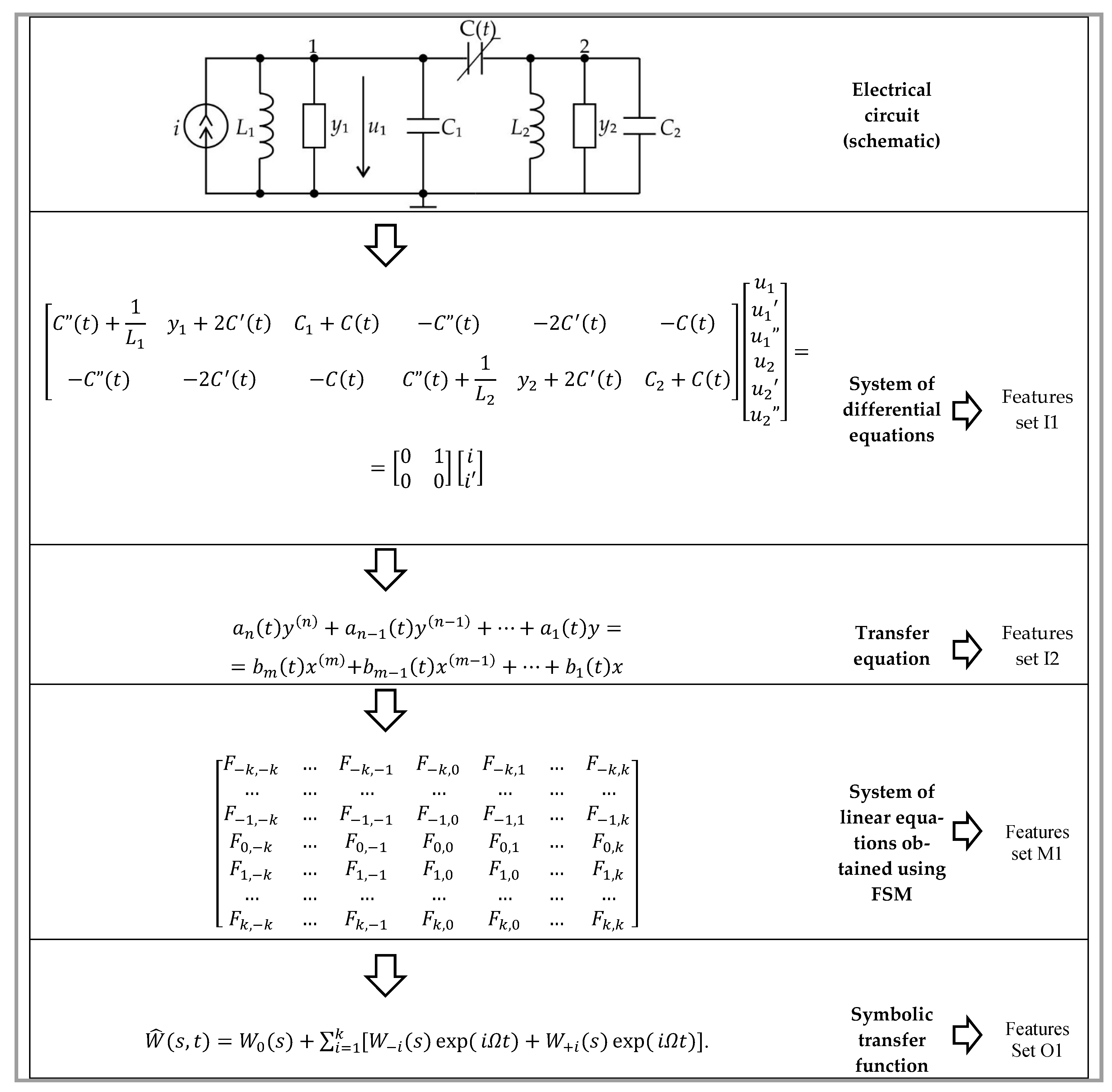
- Such an LPTV circuit in the time domain can be described by the symbolic system of linear differential equations (SSLDE).
- By eliminating internal variables in the SSLDR using one of the known methods, one can obtain a differential Equation (1) describing the circuit.where y(t) is the output (sought) and x(t) is the input (set) variable, t is the independent variable (time), and ai(t), bj(t) are parametric functions of time t.
- For an LPTV circuit described by the differential Equation (5), using the equation of L.A. Zadeh [1], we determine the differential equation describing this circuit in the frequency domain:where:is the transfer function of the LPTV circuit, and:are the corresponding time-dependent periodic functions of time t with period T coefficients of Equation (1), whereas Y(s,t) and X(s,t) are the images of the output and input variables in the frequency domain, respectively, and s is a complex variable.
- In general, Equation (6) does not have an exact analytical solution, so one must find an approximate solution that accounts for both the known properties of the desired transfer function W(s,t) and the specifics of the algorithm used for its determination:
- (a)
- The approximation Ŵ(s,t) of the transfer function W(s,t) must achieve a predefined accuracy level of choice,
- (b)
- Given that Ŵ(s,t) needs to undergo n-times differentiation when inserted into (6), it should be represented by a function that allows straightforward differentiation (i.e., intricate fractions, etc.). Consequently, for solving (6), one can suggest an approximation of the transfer function by a trigonometric Fourier series:or in a complex form:
- Regarding the choice of the number of k harmonics (step 3), it should be noted that, as a rule, the first k harmonics are typically chosen. However, there are algorithms that allow solutions to be obtained even when the number of equations is greater than the number of unknowns. In our opinion, the choice of harmonics and the number of equations in each case should be left to the specialist who designs and studies the given LPTV circuit.
- The solution obtained in step 4 of the SSLAE (in the form of M × W = P matrix) has its own peculiarities, as some or all elements of the matrix M and vector P are symbolic. Therefore, symbolic methods should be used to solve the SSLAE.
- The approximation selection of Equations (11) or (12) is not fundamentally important. However, empirical experience of using the approximation described by Equation (12), has shown that the matrix M is sparser than with approximation (11) of the same order. This is significant in the symbolic solution of the SLAP. Therefore, approximation (12) is more beneficial, in our opinion. The values of W0(s), Wci(s), Wsi(s) or W0(s), W+i(s), W−i(s) in this case are fractional rational expressions, where the denominators are identical and correspond to the determinant of the M matrix. The numerators are the determinants of the modified matrices M, where the corresponding column is replaced by the vector P.The peculiarity of steps 1–4 is that several (or even all) of the parameters of the analyzed circuit, including s, Ω, and other parametric element coefficients, are specified symbolically. Therefore, the differentiation of the approximating function, substitution of it and its derivatives into the equation (6), determination of k harmonics with (2k+1)-fold integration of the expression (13) products into the corresponding orthogonal functions, and solving the SSLAE in symbolically is very cumbersome. In this context, the sophisticated symbolic computation capabilities of contemporary CAD software (MATLAB 2014a) proved invaluable, enabling the calculations described in this manuscript to be carried out with a high degree of feasibility [15].
- The symbolic solution of the SLAE is performed in the system user-defined functions MAOPCs [15] using standard functions of the MATLAB environment.
3. Results
3.1. Consideration of Feature Extraction Required for Machine Learning Applications
- Data Collection.
- Feature Extraction (Data Conversion for applicable inputs of the ML system).
- Target Definition (what is the target of the ML system?).
- Model Selection.
- Model Training.
- Model Evaluation.
- Parameter Tuning.
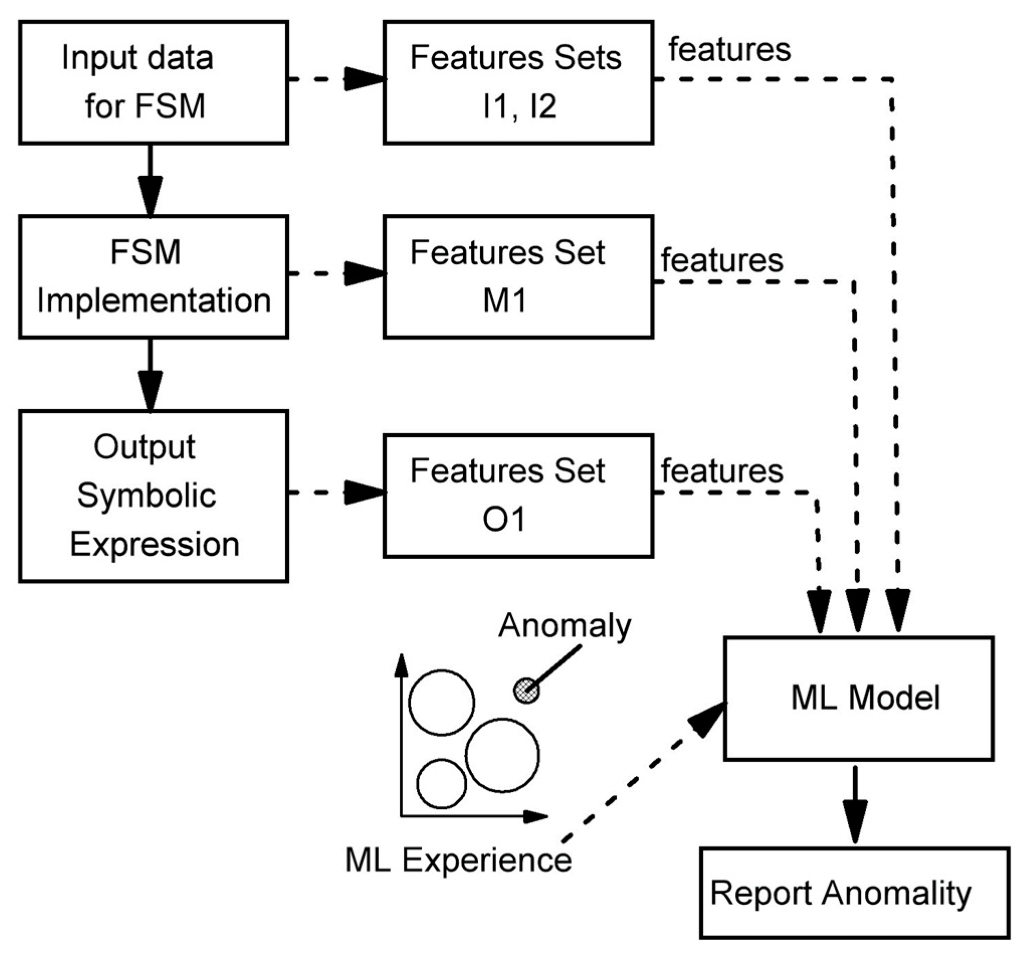
- I1 (Input type 1)—features extracted from the system of differential equations.
- I2 (Input type 2)—features extracted from the transfer equation.
- M1 (Method features 1)—features extracted from the System of Linear Algebraic Equations (SLAE) obtained using FSM.
- O1 (Output features 1)—features extracted from the symbolic transfer function obtained using FSM.
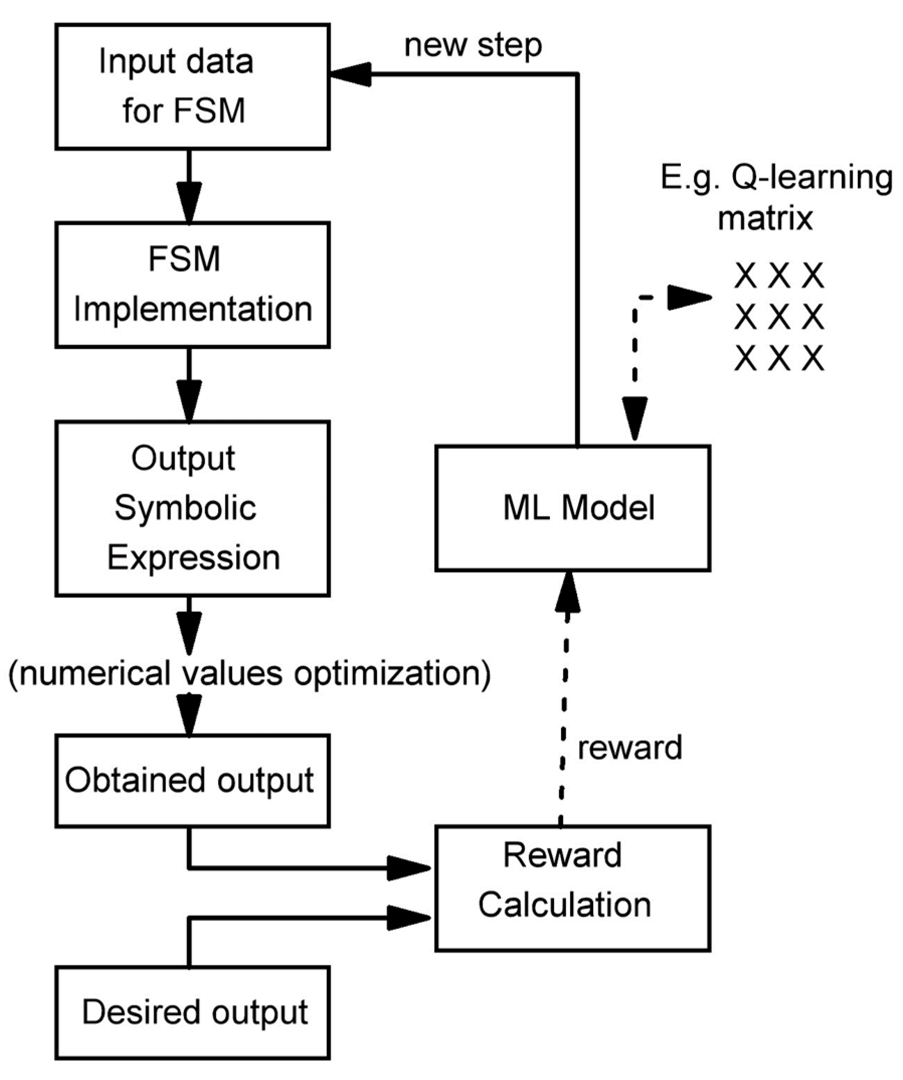
3.2. Use Case of Parametric Circuits Synthesis
- AI tries to put electronic components in a semi-random place in the schematic considering its previous experience.
- Calculate the symbolic expression of the transfer function.
- Try to optimize component values with some constraints.
- Check the best result with the target frequency characteristic and provide the corresponding “reward”.
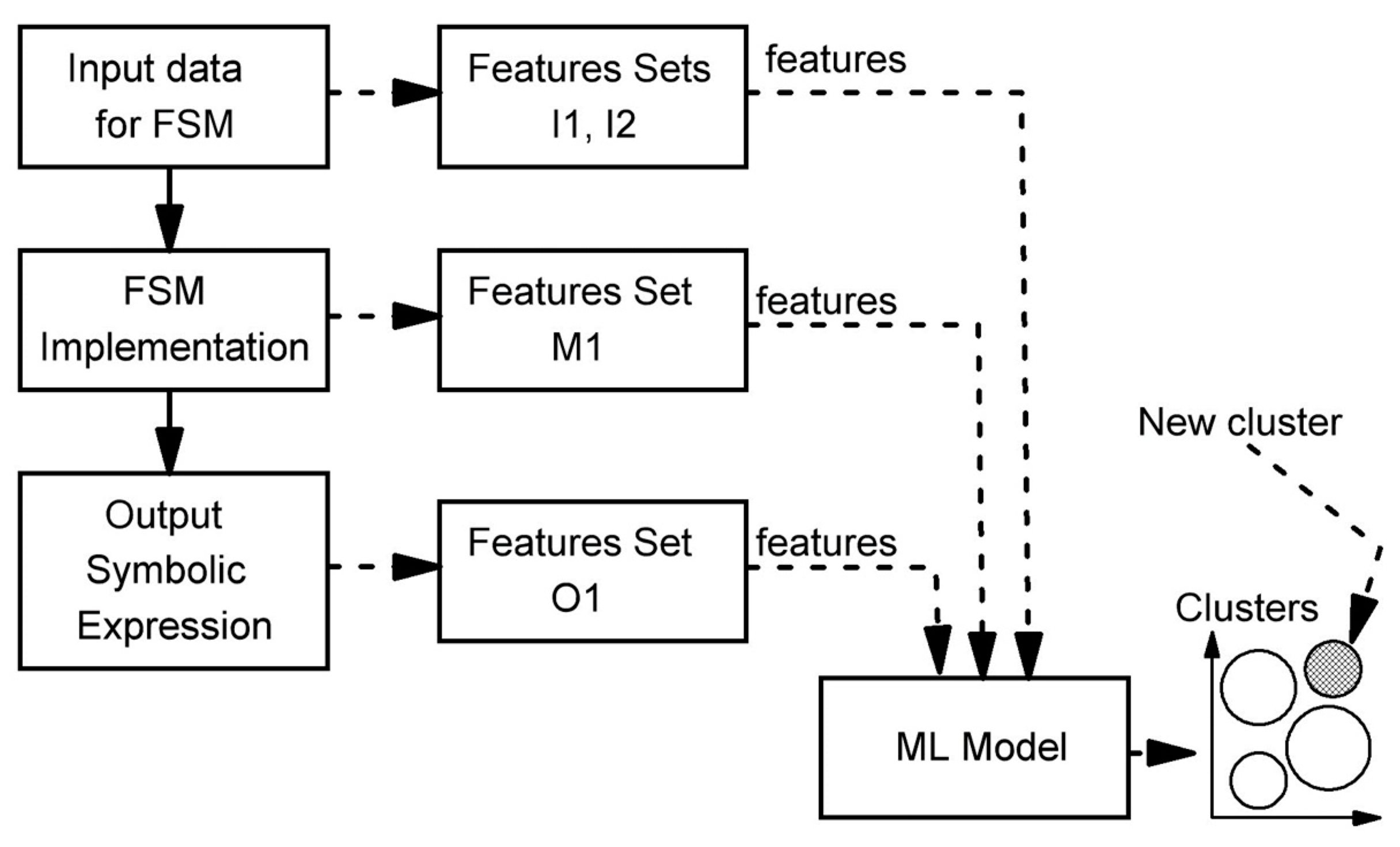
3.3. Use Case of Invisible Features Detection by Clusterization
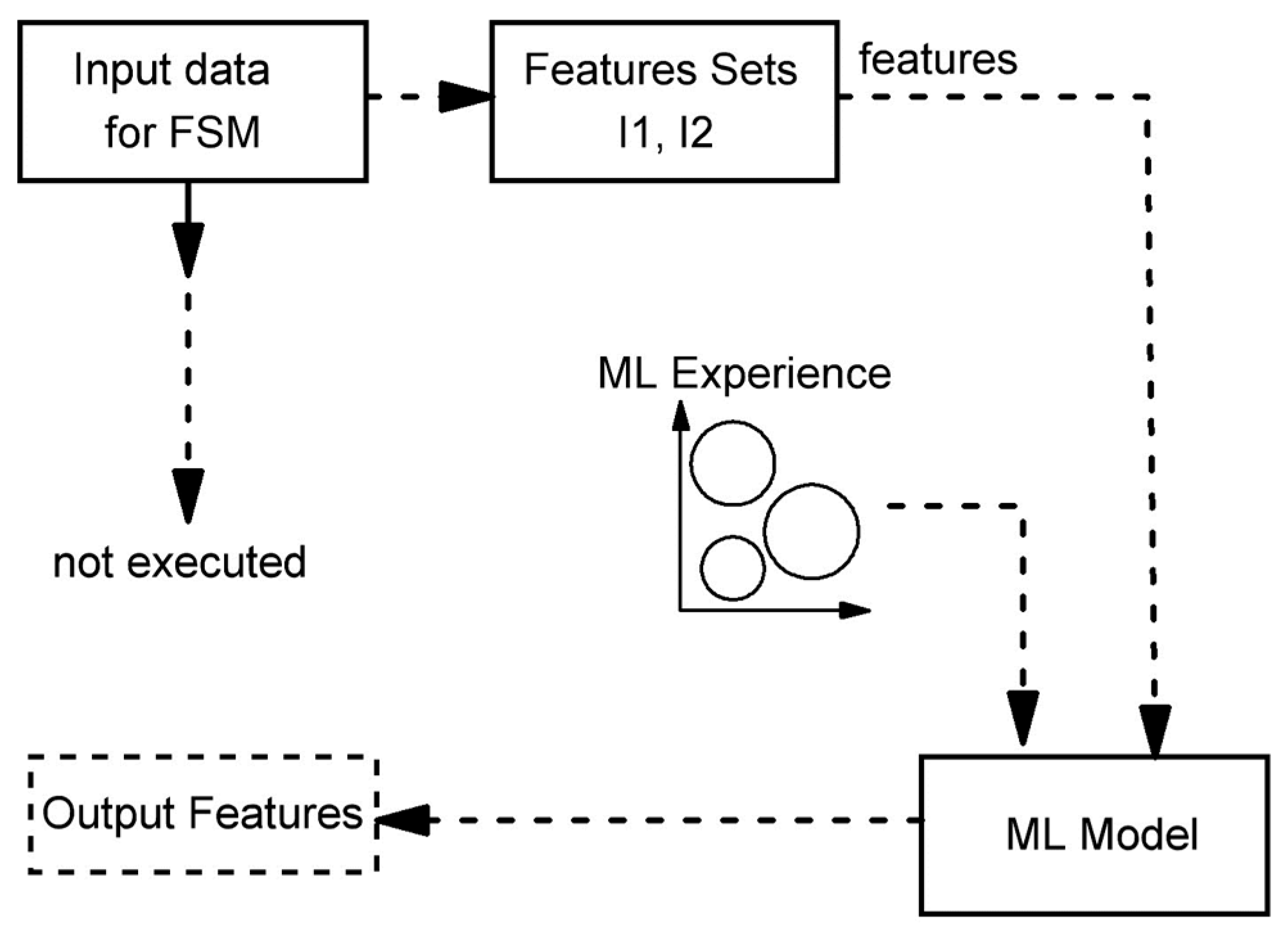
3.4. Use Case of Prediction of FSM Output
3.5. Use Case of Assistance in Frequency Symbolic Method Usage Based on Anomaly Detection
3.6. Use Case of Fault Diagnosis and Testing
- Fault Diagnosis in Electrical/Electronic Circuits:
- Predictive Maintenance: AI can be used to predict potential failures in circuits by analyzing patterns and anomalies in frequency responses. By training ML models on historical data of circuit performance, it is possible to foresee faults before they occur, allowing for proactive maintenance [13,17].
- Anomaly Detection: AI systems can be employed to detect anomalies in circuit behavior that may indicate faults. Machine learning models can learn the normal operating conditions of circuits and flag deviations from these norms, thus identifying potential issues in real-time.
- Testing and Validation:
- Automated Testing: AI-driven automated testing procedures can significantly reduce the time and effort required for validating circuit designs. By using reinforcement learning techniques, AI systems can optimize test scenarios to cover a wide range of operating conditions, ensuring robust performance.
- Simulation-Based Testing (SBT): AI can enhance simulation-based testing by rapidly generating and evaluating numerous test cases, thus providing comprehensive insights into circuit behavior under various conditions. This approach can help identify edge cases and potential weaknesses in the design.
- Parameter Tuning: AI techniques can be used to optimize the parameters of LPTV circuits. Genetic algorithms and other optimization techniques can help find the best parameter values that improve circuit performance while meeting design constraints.
3.7. Example of Symbolic Transfer Function Complexity Calculation
- Ni is number of particular operations (for i-th mathematical operand),
- wi is complexity weight of the i-th operand,
- K is total number of distinguished operands (depending on the case).
- Every number in the expression in the generic case is a complex number and it serves as our reference.
- The addition or subtraction of two complex numbers has the same complexity as two additions/subtractions of real numbers and is considered as a unit weight with value wadd = wsub = 1.
- Multiplication of two real numbers typically uses hardware acceleration, resulting in a weight of 1.
- Complex multiplication involves two multiplications and one addition, and based on the assumptions above, its weight is wmul = 3.
- The division of two complex numbers uses multiplication by the conjugate, and its weight is wdiv = 7.
- Binary exponentiation is calculated with complexity . The real and imaginary parts of the complex number are stored as 32-bit values, so = 32, therefore the weight of the exponentiation is wexp = 64.
4. Conclusions
Author Contributions
Funding
Institutional Review Board Statement
Informed Consent Statement
Data Availability Statement
Acknowledgments
Conflicts of Interest
References
- Zadeh, A. Frequency Analysis of Variable Networks. Proc. IRE 1950, 38, 291–299. [Google Scholar] [CrossRef]
- Papandreou-Suppappola, A. Applications in Time-Frequency Signal Processing; CRC Press Inc: Boca Raton, FL, USA, 2003. [Google Scholar]
- Ortigueira, M.D.; Martynyuk, V.; Kosenkov, V.; Batista, A.G. A New Look at the Capacitor Theory. Fractal Fract. 2023, 7, 86. [Google Scholar] [CrossRef]
- Ding, Y.; Deng, H.; Xie, Y.; Wang, H.; Sun, S. Time-Varying Channel Estimation Based on Distributed Compressed Sensing for OFDM Systems. Sensors 2024, 24, 3581. [Google Scholar] [CrossRef] [PubMed]
- Dhahri, S.; Naifar, O. Fault-Tolerant Tracking Control for Linear Parameter-Varying Systems under Actuator and Sensor Faults. Mathematics 2023, 11, 4738. [Google Scholar] [CrossRef]
- Jia, X.; Jiang, Y. Non-Magnetic Circulator Based on a Time-Varying Phase Modulator. Appl. Sci. 2023, 13, 512. [Google Scholar] [CrossRef]
- Grabowski, D.; Maciążek, M.; Pasko, M.; Piwowar, A. Time-invariant and time-varying filters versus neural approach applied to DC component estimation in control algorithms of active power filters. Appl. Math. Comput. 2017, 319, 203–217. [Google Scholar] [CrossRef]
- Eom, B.H.; Day, P.K.; LeDuc, H.G.; Zmuidzinas, J. A wideband, low-noise superconducting amplifier with high dynamic range. Nat. Phys. 2012, 8, 623–627. [Google Scholar] [CrossRef]
- Wiechetek, K.; Piskorowski, J. A Concept of the Non-Stationary Filtering Network with Reduced Transient Response. Appl. Sci. 2019, 9, 4570. [Google Scholar] [CrossRef]
- Zhang, H.; Guoan, B.; Zhao, L.; Razul, S.G.; See, C.-M.S. Time varying filtering and separation of nonstationary FM signals in strong noise environments. In Proceedings of the IEEE International Conference on Acoustics, Speech and Signal Processing, Florence, Italy, 4–9 May 2014; pp. 4171–4175. [Google Scholar] [CrossRef]
- Ou, B.; Liu, D. Chaotic attractor generation via a simple linear time-varying system. Discret. Dyn. Nat. Soc. 2010, 2010, 840346. [Google Scholar] [CrossRef]
- Kocoń, S.; Piskorowski, J. Time-Varying IIR Notch Filter with Reduced Transient Response Based on the Bézier Curve Pole Radius Variability. Appl. Sci. 2019, 9, 1309. [Google Scholar] [CrossRef]
- Golonek, T.; Chruszczyk, Ł. Analog Circuits Specification Driven Testing by Means of Digital Stream and Non-Linear Estimation Model Optimized Evolutionarily. Bull. Pol. Acad. Sci. Tech. Sci. 2020, 68, 1283–1299. [Google Scholar] [CrossRef]
- Yin, Z.; Jiang, X.; Zhang, N.; Zhang, W. Stability Analysis for Linear Systems with a Differentiable Time-Varying Delay via Auxiliary Equation-Based Method. Electronics 2022, 11, 3492. [Google Scholar] [CrossRef]
- Shapovalov, Y.; Bachyk, D.; Detsyk, K. Multivariate Modelling of the LPTV Circuits in the MAOPCs Software Environment. Prz. Elektrotech. (Electr. Rev.) 2022, 98, 158–163. [Google Scholar] [CrossRef]
- Polyanin, A.D.; Zaitsev, V.F. Handbook of Exact Solutions for Ordinary Differential Equations, 2nd ed.; Chapman & Hall/CRC: Boca Raton, FL, USA, 2003. [Google Scholar]
- Pawełczyk, R.; Grzechca, D. Improvement of functional safety of the level crossing barrier machine by a noninvasive angle detection method. IEEE Des. Test 2022, 39, 43–53. [Google Scholar] [CrossRef]


| Feature ID and Short Name | Description | Data Type | Valid Range |
|---|---|---|---|
| I1.1 Number of LC components | Number of LC components (except parametric) in the system of differential equations describing the circuit. | Numerical | Positive integer number |
| I1.2 Percentage of non-zero elements | Relation of non-zero elements to all elements. | Numerical | Positive integer [0, 100] |
| I1.3 Count of symbolic parameters | Total number of parameters in symbolic form. | Numerical | Positive integer number |
| I1.4 Percentage of symbolic cells to the numerical cells | Relation of cells number in the system of differential equations containing at least one symbolic variable to the total number of cells. | Numerical | Positive integer [0, 100] |
| I1.5 Time-varying function type | Time-varying function type as one of single harmonic, bi-harmonic, multi-harmonic, etc. | Categorical | [Harm, biharm, multiharm] |
| Feature ID and Short Name | Description | Data Type | Valid Range |
|---|---|---|---|
| I2.1 Order of the left part | Order of the left part of the transfer equation. | Numerical | Positive integer number |
| I2.2 Order of the right part | Order of the right part of the transfer equation. | Numerical | Positive integer number |
| I2.3 Count of symbolic parameters | Total number of parameters in symbolic form. | Numerical | Positive integer number |
| I2.4 Complexity of expression | Numerical value representing the complexity of the symbolic expression. For example, a function depending on the number of multiplications, exponents, logarithmic operation, and so on. | Numerical | Positive integer number 1 |
| Feature ID and Short Name | Description | Data Type | Valid Range |
|---|---|---|---|
| M1.1 Order of the SLAE (2k + 1) | Order of the SLAE obtained using FSM. | Numerical | Positive integer number |
| M1.2 Complexity of SLAE | Numerical value representing the complexity of SLAE, i.e., some functions depend on the average complexity of cells in SLAE. The complexity of each SLAE cell could be calculated as binary expression tree complexity. | Numerical | Positive integer number 1 |
| Feature ID and Short Name | Description | Data Type | Valid Range |
|---|---|---|---|
| O1.1 Number of terms in the transfer function | Number of terms in the transfer function. | Numerical | Positive integer number |
| O1.2 Complexity of transfer function | Numerical value representing the complexity of the transfer function. For example, some functions depend on the average complexity of each term. | Numerical | Positive integer number 1 |
| O1.3 Maximal complexity of one term | Numerical value representing the complexity of the most complex term in the transfer function. For example, some functions depend on the number of multiplications or exponentiations of symbolic variables. | Numerical | Positive integer number 1 |
| Target ID and Short Name | Description | Data Type | Valid Range |
|---|---|---|---|
| T1.1 Integral deviation of obtained transfer function from desired | Integral deviation of the obtained transfer function from desired. It is obtained after substitution of the numerical values (may be also optimization applied) into the symbolic transfer function and integral comparison with the target transfer function. | Numerical | Floating-point number |
| T1.2 Local deviation of obtained transfer function from desired | Like above but evaluated in a specified local range of time or frequency. | Numerical | Floating-point number |
| T1.3 Amplification possibility | Is it possible that module of transfer function causes signal amplification? | Categorical | [“Yes”, “No”]. |
| T1.4 Possible non-stability | Is the non-stability of the system/circuit possible? | Categorical | [“Yes”, “No”] |
| Operation | Weight |
|---|---|
| add | 1 |
| sub | 1 |
| mul | 3 |
| div | 7 |
| exp | 64 |
| Operation | Number of Operations | Cost |
|---|---|---|
| add | 48 | 48 |
| sub | 33 | 33 |
| mul | 67 | 201 |
| div | 3 | 21 |
| exp | 44 | 2816 |
| Total 3119 |
| Operation | Number of Operations | Cost |
|---|---|---|
| add | 240 | 240 |
| sub | 238 | 238 |
| mul | 433 | 1299 |
| div | 5 | 35 |
| exp | 373 | 23,872 |
| Total 25,684 |
| Operation | Number of Operations | Cost |
|---|---|---|
| add | 722 | 722 |
| sub | 626 | 626 |
| mul | 1213 | 3639 |
| div | 7 | 49 |
| exp | 1081 | 69,184 |
| Total 74,220 |
| Use Case | Benefit | Learning Type | Difficulties/Problems |
|---|---|---|---|
| Parametric circuits synthesis | Circuit could be synthesized automatically. | Reinforcement learning | Could be time consuming. Big database is needed for ML experience storage. |
| New features detection | Identify not visible features of the FSM method or its implementation by specific clusters occurrences. | Unsupervised learning | At the moment, it is not clear which clusters could be obtained. |
| Prediction | Could predict the result based on previous experience without modeling and simulation. | Supervised learning | For some not typical inputs, the result could be predicted incorrectly. |
| Anomaly detection | Human mistakes could be detected. This use case acts as an assistant. | Supervised learning | Could accidentally report an anomaly when the correct approach is used. |
Disclaimer/Publisher’s Note: The statements, opinions and data contained in all publications are solely those of the individual author(s) and contributor(s) and not of MDPI and/or the editor(s). MDPI and/or the editor(s) disclaim responsibility for any injury to people or property resulting from any ideas, methods, instructions or products referred to in the content. |
© 2024 by the authors. Licensee MDPI, Basel, Switzerland. This article is an open access article distributed under the terms and conditions of the Creative Commons Attribution (CC BY) license (https://creativecommons.org/licenses/by/4.0/).
Share and Cite
Shapovalov, Y.; Mankovskyy, S.; Bachyk, D.; Piwowar, A.; Chruszczyk, Ł.; Grzechca, D. Machine Learning Use Cases in the Frequency Symbolic Method of Linear Periodically Time-Variable Circuits Analysis. Appl. Sci. 2024, 14, 7926. https://doi.org/10.3390/app14177926
Shapovalov Y, Mankovskyy S, Bachyk D, Piwowar A, Chruszczyk Ł, Grzechca D. Machine Learning Use Cases in the Frequency Symbolic Method of Linear Periodically Time-Variable Circuits Analysis. Applied Sciences. 2024; 14(17):7926. https://doi.org/10.3390/app14177926
Chicago/Turabian StyleShapovalov, Yuriy, Spartak Mankovskyy, Dariya Bachyk, Anna Piwowar, Łukasz Chruszczyk, and Damian Grzechca. 2024. "Machine Learning Use Cases in the Frequency Symbolic Method of Linear Periodically Time-Variable Circuits Analysis" Applied Sciences 14, no. 17: 7926. https://doi.org/10.3390/app14177926
APA StyleShapovalov, Y., Mankovskyy, S., Bachyk, D., Piwowar, A., Chruszczyk, Ł., & Grzechca, D. (2024). Machine Learning Use Cases in the Frequency Symbolic Method of Linear Periodically Time-Variable Circuits Analysis. Applied Sciences, 14(17), 7926. https://doi.org/10.3390/app14177926