Abstract
The fluctuating pressure acting on the radial gate in the high-head flood discharge outlet is the main excitation source of flow-induced vibration. Therefore, this paper delves into the distribution characteristics of fluctuating pressure on the panel of the high-head submerged radial gate based on hydraulic model tests. Hydraulic tests were first conducted to obtain the distribution patterns of time-averaged pressure and the root mean square (RMS) of fluctuating pressure on the radial gate panel. Secondly, the improved complete ensemble empirical mode decomposition with adaptive noise (ICEEMDAN) and HHT method was employed to identify the causes of the fluctuating pressure on the gate panel. Finally, the ICEEMDAN-SSA (the sparrow search algorithm)–LSTM (long short-term memory) method was utilized to achieve accurate prediction of the fluctuating pressure on the gate panel. The results show that the time-averaged pressure in the middle of the gate panel is higher than that at the top and near the bottom edge, which differs significantly from the static pressure distribution. The RMS of the fluctuating pressure near the bottom edge is higher than that in the middle and at the top. The fluctuating pressure acting on the gate panel in the time domain can be regarded as a stationary process. The fluctuating pressure on the gate panel is caused by the combined diffusion and random mixing of multi-scale vortices in the turbulent eddy structure. The ICEEMDAN-SSA-LSTM combined method significantly improves the prediction accuracy of fluctuating pressure on the gate panel compared to the LSTM and ICEEMDAN-LSTM methods.
1. Introduction
The considerable quantity of energy conveyed by the flood discharge and the intricate attributes of the high-speed water flow render the flood discharge vibration problem particularly pronounced. The hydraulic steel gate plays a pivotal role in regulating water discharge structures in hydraulic and hydropower engineering [1]. Its safe and flexible operation determines the success of the entire project and the safety of downstream people and property [2]. The development of gates is trending towards larger scales and lighter weights to meet the demands of high water heads, large orifices, and large discharge flows. Fluid-induced vibration (FIV), dynamic stability, and the safety and reliability of hydraulic gate structures under dynamic water action have received increasing attention from the water conservancy engineering community [3]. Due to the complex fluid–structure interaction (FSI), there are cases where the gate does not function properly or even becomes destabilized due to vibration [4]. The intelligent regulation of hydropower stations, which requires the gate to be partially opened in dynamic water, leads to complex operating conditions. FIV caused by flood discharge is the main cause of the dynamic instability of radial gates [5,6].
The radial gates of discharge structures are primarily installed in spillways with low water heads and bottom outlets with high water heads. The front section of a high-head bottom outlet typically constitutes a pressurized section, where water flow through the pressure slope is regulated by the gate, transitioning from pressurized flow to open channel flow [7]. The submerged radial gate is often chosen as the type of pressurized outlet gate due to its ability to regulate flow stably. Following the pressurized section outlet radial gate, it is typically designed with a bottom drop and sudden lateral enlargement. This design feature helps protect the chute bottom and side walls from cavitation erosion by facilitating appropriate aeration [8,9]. In this type of configuration, the bottom slope is typically steeper, and the flow velocity increases after passing through the gate [10], resulting in a typical open channel flow condition. This flow condition is significantly different from a submerged hydraulic jump, meaning that the water body downstream of the gate has a negligible impact on the vibration of the gate. Instead, the fluctuating water pressure acting on the gate panel is the direct cause of vibration [11].
The current state of research about gate vibration in high-head bottom outlets can be broadly categorized into three main aspects: prototype testing, hydraulic experiments, and numerical simulation. Yan et al. [12] conducted a prototype test on the high-head and large-dimension gate in the emptying culvert of the Tianshengqiao power station. The variation patterns of flow fluctuating pressure and structural vibration parameters with gate opening indicated that the gate structure should avoid operation in a small gate opening (n = 0~0.1) and large gate opening (n = 0.7~0.9) to prevent cavitation erosion and fatigue damage to the building structure. Lian et al. [13] elucidated the causes and mechanisms of the accompanying vibration of radial gates through prototype observations conducted at the Jinping hydropower station. Their findings suggested that the vibration of the mid-level orifice gate was attributed to the FSI between the gate and the turbulent flow fluctuating pressure. This vibration was subsequently transmitted through the dam body to the surface orifice gate, where it was amplified to a certain extent, resulting in significant vibrations of the surface orifice. Zhang et al. [14] conducted hydraulic experiments and three-dimensional finite element simulations to investigate the hydraulic characteristics, static and dynamic characteristics, dynamic stability, and FIV characteristics of submerged radial gates. The study indicated that the fluctuating pressure at the same position gradually increases with increasing gate openings, and the primary energy distribution occurs within the range of 10 Hz, with a dominant frequency below 1 Hz. Lee [15] proposed a method to mitigate the flow-induced vibration of a radial sluice gate to ensure operational safety and long-term stability. Simulation analysis demonstrated that the vertical vibration acceleration of the gate decreased by 70% after attaching the supplementary plate. Daneshmand et al. [16] utilized a combined physical and numerical method to study the pressure characteristics of the radial gate plane at the bottom outlet of the Shahryar Dam in Iran. The measurements revealed that the pressure fluctuations in the current scenario were random in the time domain. Furthermore, the results from the hydraulic model experiment indicated that the fundamental frequency of the service radial gate was sufficiently far from the dominant frequencies in the power spectral density of the fluctuating pressure, thus mitigating the risk of resonance for the gate.
The hydrodynamic pressure exerted on the radial gate panel significantly affects the gate’s safe operation. Wang et al. [17] developed a semi-empirical and semi-theoretical formula for hydrodynamic pressure acting on the radial gate panel, taking into account the characteristics of hydrodynamic pressure and considering the influence of hinge position and rotating arm radius on panel hydrodynamic pressure. In the context of partial opening conditions, the method for calculating panel hydrodynamic pressure for radial gates primarily relies on the principle of potential flow. Currently, there have been few studies conducted on the theoretical calculation of hydrodynamic pressure for radial gates. These studies are typically based on the principles of hydrostatic pressure and potential energy, supplemented by a hydrodynamic pressure function [18]. Theoretical calculations often fail to accurately predict turbulence intensity during gate discharge due to the inherent turbulence in real-world situations. Consequently, it becomes challenging to determine the hydrodynamic pressure characteristics of radial gates, such as fluctuating pressure and other variations, leading to lower theoretical calculation accuracy. As a result, only conservative pressure values can be obtained, limiting the study of gate stability and potentially leading to unsuitable material and structural designs.
In addition, the turbulent nature of water flow in the discharge process of hydraulic radial gates poses challenges for direct simulation and calculation. With the emergence of artificial intelligence in various fields, data-driven machine learning techniques have become a focal point in turbulence research, attracting numerous experts and scholars to investigate. Gang et al. [19] employed machine learning techniques to predict wind pressures around circular cylinders. The results suggested that gradient-boosting regression tree models offer an efficient and economical alternative to traditional wind tunnel tests and computational fluid dynamics simulations for determining wind pressures around two-dimensional smooth circular cylinders. G. Sudharsun et al. [20] utilized machine learning techniques to concentrate on modeling the fluctuating pressure rate of strain tensor in turbulent flows and quantifying uncertainties in the Reynolds stress model.
Currently, fluctuating signals (such as fluctuating pressure, vibration acceleration, vibration stress, etc.) are often predicted directly from the original time series of the signal. This method does not thoroughly investigate the formation mechanism of fluctuating signals, and the accuracy needs further improvement. Therefore, it is necessary to perform decomposition preprocessing of the fluctuating signals before prediction. Traditional methods like empirical mode decomposition (EMD), ensemble empirical mode decomposition (EEMD), complete ensemble empirical mode decomposition (CEEMD), and complete ensemble empirical mode decomposition with adaptive noise (CEEMDAN) have drawbacks such as mode mixing, poor adaptability, and stability issues [21]. Additionally, traditional neural network models like Back Propagation (BP), recurrent neural network (RNN), and Radial Basis Function (RBF) algorithms have disadvantages, such as slow training speeds and susceptibility to local optima. The long short-term memory (LSTM) model can overcome these shortcomings, offering advantages, such as fast convergence speed and high computational accuracy, and it has been widely applied in regression testing and model prediction fields [22]. It is noteworthy that parameter optimization of the LSTM neural network significantly impacts prediction accuracy. Therefore, existing studies have often focused on either single data series decomposition or the initial parameter optimization of the LSTM model [23], while research combining these two aspects to study the fluctuating load of water flow is relatively scarce.
In conclusion, the limited understanding of the physical mechanisms governing fluctuating flow has constrained research into hydrodynamic pressure in the discharge process of radial gates, thereby impacting studies on FIV and dynamic stability. This paper addresses these challenges by constructing a large-scale submerged radial gate model at a 1:25 length scale. Through extensive experimentation, the fluctuating pressure on the submerged radial gate plane was systematically investigated, and the distribution characteristics of time-averaged pressure and RMS of fluctuating pressure on the gate panel were analyzed. Additionally, the generation mechanism of fluctuating pressure on the gate panel was explored using the improved ICEEMDAN-HHT method. Furthermore, ICEEMDAN-SSA-LSTM was employed to predict panel fluctuation on submerged radial gate panels, offering valuable insights for engineering design and operation.
2. Methodology
2.1. Principle of the CEEMDAN Algorithm
In this paper, we introduce the improved HHT based on ICEEMDAN for gate panel fluctuating pressure in order to capture fluctuating characteristics at different vortex scales. The ICEEMDAN algorithm is based on EMD. To address mode aliasing and the issue of many small-amplitude IMF components in the original EMD algorithm, the ICEEMDAN algorithm adds Gaussian white noise during the decomposition iteration. This process enhances anti-interference capability and partially solves the aforementioned problems. Compared with the complete ensemble empirical mode decomposition with adaptive noise (CEEMDAN) algorithm, which uses the average of the IMF decomposed by multiple noisy signals as the IMF for each iteration [24], the ICEEMDAN algorithm uses the residuals of the previous iteration minus the average of residuals of multiple noisy signals of the current iteration as the IMF for the original signal iteration, which can further alleviate the phenomenon of noise residuals in the IMF, as well as the problem of modal mixing, and improve the decomposition effect. Therefore, in order to improve the analysis of time series, this paper uses the ICEEMDAN algorithm instead of the EMD used in HHT.
Based on the EMD algorithm, ICEEMDAN adds a special white noise ηi with mean 0 and variance 1 to the decomposition process to decompose the signal x(t) into several IMF components and a residual function component. The ICEEMDAN method effectively mitigates the problems of residual noise and mode aliasing that may exist in the IMF of the EMD and EEMD algorithms. The ICEEMDAN decomposition process is as follows:
- (1)
- The operator in EMD decomposes the original signal in kth mode, and the operator is used to generate the local mean of the signal.
- (2)
- Construct the additive noise signal and compute the first-order residual . Where is added at the initial stage to remove noise and is the inverse of desired signal-to-noise ratio between the first additive noise signal and the analyzed signal. i denotes the number of times the noise is added, std denotes the standard deviation, and the operator denotes averaging over the whole.
- (3)
- When k = 1, the 1st IMF component is calculated as follows: .
- (4)
- The 2nd residuals and IMF components are obtained using the average of local means as follows:
- (5)
- Derivation of the kth mode is as follows:
- (6)
- Repeat step 5 to obtain all residuals and IMF components.
2.2. Principle of the HHT Algorithm
HHT, proposed by Huang E. et al. [25], is a novel method utilized for analyzing non-smooth and non-linear signals. The method consists of two main components: EMD and Hilbert Transform (HT) with its spectral analysis, with EMD being the primary component. HHT initially decomposes the signal adaptively into a series of IMFs through EMD. Subsequently, it performs HT on each IMF to extract the physically meaningful instantaneous frequency and instantaneous amplitude, enabling the observation of the signal’s frequency domain characteristics over time. Unlike traditional signal processing methods, HHT does not require prior analysis or research or the establishment of basis functions. Instead, it employs an adaptive decomposition of the original signal into the sum of several IMFs based on its intrinsic properties [26]. Each IMF component represents a specific frequency component in the original signal and is decomposed sequentially from high frequency to low frequency. For a random temporal signal , the HT yields the following result:
where is the Cauchy principal value. In this way, the analytic signal of the original timing signal can be constructed from the mutually complex conjugates and as follows:
These functions contain information about the amplitude and phase of the signal. represents the amplitude function, while represents the phase function of the signal.
The instantaneous amplitude and instantaneous frequency obtained by HT are functions of time. When the amplitude is expressed as a function of time and frequency, the time–frequency distribution spectrum of the amplitude is obtained, which is called the Hilbert spectrum, denoted as . The integration over time for yields the Hilbert marginal spectrum as follows:
The Hilbert marginal spectrum accumulates the amplitude at each frequency over the entire time period, representing the global contribution of energy (or amplitude) at each frequency. It reflects the cumulative amplitude of all the data in a statistical sense [24]. The marginal spectrum of the fluctuating pressure signal accurately represents the actual frequency components of the signal, with the peak of the marginal spectrum corresponding to the dominant frequency.
2.3. Principle of the SSA Algorithm
SSA is a novel swarm intelligence algorithm [27]. In SSA, a group of sparrows imitates the foraging behavior of real sparrows. Some sparrows serve as scouts, scouting foraging areas and providing directions to the entire group, while the remaining sparrows act as followers, relying on the scouts to find food. Sparrows only have positional attributes, and during foraging, the roles of scout and follower can interchange, but the total number and proportions of sparrows in each role remain constant. Sparrows on the periphery of the group emit alarms when they detect danger, prompting the entire group to move to a safer area if the alarm value exceeds a certain threshold. When optimizing with SSA, the positional update of the scouts during iterations can be expressed as follows:
where and are the jth dimensional position information of the ith sparrow at iteration number K and K+1, respectively; a is a random number within 0~1; is the maximum iterations; Q is a random number obeying a normal distribution; L is a matrix of type 1×d with all elements of 1 (d is the dimension of feature); is the alarm value, ; and ST is the safe value, .
When , there are no predators in the foraging environment, and the discovers can conduct forage extensively; the sparrow position will be updated based on the current solution in an exponential decay manner, which reduces the value of the solution by multiplying by . When , certain sparrows detect predators and sound an alarm, prompting the sparrow group to migrate to a safe area.
The sparrow positions will then be updated based on the current solution and Q. The expression for the position of the follower flying to the center when is as follows:
where Xw is the worst position; is the current optimal position of the discover; A is a matrix of type 1 × d with elements randomly assigned to 1 or −1 and satisfying the relation ; and n is the number of followers.
When , if the ith follower is less adapted and unable to forage, the sparrow group needs to fly elsewhere to obtain food. During the course of group activity, once the danger is perceived by a marginal sparrow, the anti-predator behavior is initiated as follows:
where is the global optimal position; α and β are the control step parameters; ε is a constant to avoid a denominator of 0; is the adaptation of the ith follower; is the optimal adaptation; and is the worst adaptation.
2.4. Principle of the LSTM Algorithm
The LSTM model, introduced by Hochreiter and Schmidhuber in 1997 [28], is a type of recurrent neural network (RNN) designed for temporal data with a chain-like structure similar to traditional RNNs. In RNNs, the self-connected hidden layer creates dependencies that require updating the hidden layer state at the current time step based on the previous one. However, RNNs encounter challenges when handling long time series data due to the potential for exponential growth or decay of gradients through repeated multiplications, leading to issues such as gradient vanishing or exploding during training. The LSTM model overcomes this inherent limitation of RNNs by preserving early time series information. While the hidden layer of LSTM retains the self-connection structure, it introduces three types of gate mechanisms (“forget gate”, “input gate”, and “output gate”) to control the flow and update of cell state and hidden layer state information. This effectively addresses problems, like gradient vanishing or exploding, that arise when processing time series data [29]. The hidden layer structure of LSTM is depicted in Figure 1.
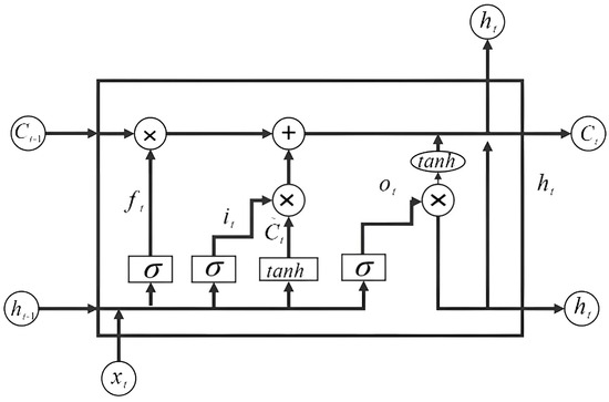
Figure 1.
The LSTM hidden layer structure.
In Figure 1, is the input signal; is the output signal at time t − 1; is the output value; is the output signal of the “input gate”, which also indicates the new memory cell; represents the cell state information at time t − 1; and represents the final memory cell information of the current layer. , , and are the control coefficients corresponding to the “forget gate”, “input gate”, and “output gate” structures, respectively, and σ is the sigmoid activation function.
The “forget gate” determines whether or not to transfer the cell state information from the previous moment to the current moment. The cell state information at moment t−1 is determined based on , as illustrated in Figure 1. When is close to 0, it is completely forgotten; conversely, when is close to 1, it is completely retained. The “input gate” can control how much new information needs to be added to the cell state through a sigmoid activation function. The “output gate” determines the effect of the current cell state on the state and output of the hidden layer, and the output is determined by a sigmoid activation function. The expression of LSTM is as follows:
where, Wf, Wi, We, and Wo are weight matrices, bf, bi, bc, and bo are biases, and tanh is the hyperbolic tangent activation function.
3. Experiment Setup and Data Acquisition
3.1. Experiment Setup
The bottom outlet consists of an inlet section, a pressurized section, and an open channel section. At the tail of the horizontal section, there is a 20 m long pressurized slope section with a slope ratio of 1:5. The cross-sectional size tapers from 5.5 m × 12 m (width × height) to 5.5 m × 8 m, with a radial gate of 5.5 m × 8 m (width × height) set at the end of the pressurized section. The model arrangement is depicted in Figure 2. In the notation used, H represents the upstream reservoir level minus the height of the bottom plate, while e denotes the relative opening of the gate, defined as e = h/ho. This ratio is illustrated schematically in Figure 3.
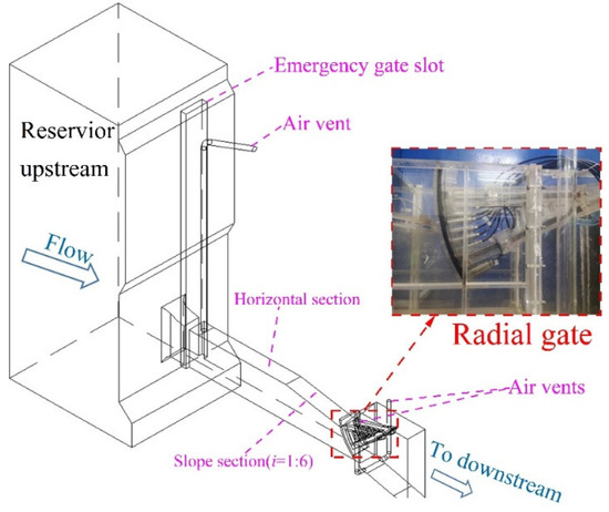
Figure 2.
Model layout.
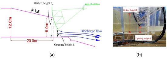
Figure 3.
Partial opening diagram. (a) Gate opening diagram; (b) gate opening schematic diagram.
The scale ratio of 1:25 is chosen based on the gravity similarity criterion. The scale of this model is 1:25, with a model flow velocity exceeding 6 m/s. The Reynolds number of the gate section significantly surpasses 1 × 10⁵, indicating that the water in the bottom outlet is in a fully turbulent state. Therefore, the scale effect produced by viscous stress can be disregarded [30]. Both the model and the radial gate were constructed from transparent Plexiglas to facilitate the observation of flow details. The results presented in this paper represent prototype values obtained by converting all model test results using the appropriate scaling factors. The input experimental parameters can be found in Table 1.

Table 1.
The input experimental parameters.
3.2. Data Acquisition
Fluctuating pressure was measured using the CY301 high-precision digital fluctuating pressure sensor by Chengdu TST in China, along with its accompanying acquisition software Smartsensor 4.30. The sensor is equipped with features, such as filtering and correction, which are applied to the pressure signal captured by its sensitive components. It directly outputs digital signals that can be displayed and stored without the need for additional data acquisition equipment. Moreover, it can be easily connected to a computer, enabling direct reading of the pressure value on the computer. Following the sampling theorem, the fluctuating pressure sampling frequency was set to 50 Hz, with a sampling duration of 20.48 s, resulting in 1024 discrete points.
To examine the distribution of fluctuating pressure on the gate panel, seven pressure measurement points are arranged on the gate panel, as depicted in Figure 4. The convenient installation of the pressure sensor and the structural arrangement of the main beam of the gate allow for the positioning of measuring points P1, P3, P5, and P7 along the centerline. Points P2, P4, and P6 are located 0.8 m away from the centerline.
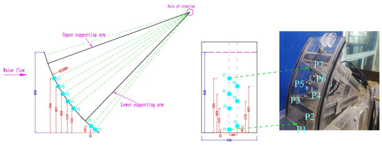
Figure 4.
Layout of pressure measurement point (unit: mm).
4. Pressure Characteristics on the Gate Panel
4.1. The Pressure Distribution Characteristics on the Gate Panel
4.1.1. Pressure Time-Domain Analysis
Figure 5 shows the time-domain process of the seven pressure measurement points on the radial gate model at e = 10%, with H = 79.0 m. It can be observed in the figure that the amplitude of the time-domain process at each measurement point is markedly different, yet they all exhibit pronounced fluctuations.
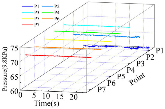
Figure 5.
Pressure distribution of the gate panel measuring points (e = 10%, H = 79 m).
There is no universal standard for distinguishing between Gaussian and non-Gaussian water pressure distributions for practical applications. In the present study, Gioffre et al. [31] proposed the criteria kurtosis coefficient (CE) > 3.5 and skewness coefficient (CS) > 0.5 to define the area of deviation from the Gaussian distribution. As depicted in Figure 6, the CE of the two typical measurement points exceeds 3, indicating that the overall data distribution is steeper and more concentrated in the center. However, the CS of the two measurement points exhibit one value greater than 0 and one less than 0. This analysis suggests that the fluctuating pressure exhibited by the gate panel is consistent with a normal distribution.
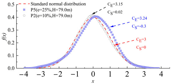
Figure 6.
Typical probability density distribution of measurement points.
The amplitude and distribution pattern of fluctuating pressure serve as the basis for calculating dynamic loads in the design of structures [32]. Typically, the RMS value of fluctuating pressure is used to describe it, which reflects the energy or intensity of the signal.
Figure 7 illustrates the pressure distribution characteristics at points near the bottom edge for various gate openings. Points 1 and 2 demonstrate a pattern of initial decrease, followed by an increase and then a subsequent decrease as the gate opening degree increases. With the exception of openings at 90%, it is evident that as the gate opening increases, the root mean square (RMS) of the fluctuating pressure at points 1 and 2 gradually rises. This indicates that the fluctuation intensity of the flow near the bottom edge increases with the increasing gate opening. Furthermore, additional analysis reveals that the rise in the RMS at the measurement points is minimal when the gate opening is less than 65% but becomes pronounced when the opening exceeds 70%. These findings suggest that as the gate opening increases, the turbulence of the water body near the bottom edge becomes more prominent.
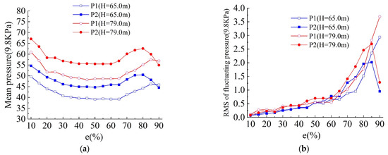
Figure 7.
Pressure distribution at measuring points near the bottom edge of the gate at different openings: (a) time-average pressure; (b) fluctuating pressure.
Figure 8 illustrates the pressure distribution characteristics at seven measurement points on the gate panel under five different upstream water levels. Contrary to the pressure near the bottom edge (P1 and P2), as well as in the middle and upper portions, it is evident that the time-averaged pressure on the panel is higher in the center under each water level (P3, P4, and P5). It is worth noting that the aforementioned distribution differs significantly from the gate’s hydrostatic pressure distribution. This discrepancy arises from the considerably higher velocity near the bottom, as per Bernoulli’s equation, leading to a lower pressure head at the bottom compared to the middle. As depicted in Figure 8b, the RMS of fluctuating pressure near the bottom is substantially higher than that in the middle and the top, indicating a higher fluctuating pressure near the bottom compared to the middle and the top.
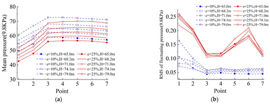
Figure 8.
Pressure distribution at measuring points of the gate panel at different upstream reservoir levels: (a) time-average pressure; (b) fluctuating pressure.
Moreover, the combination of Figure 7 and Figure 8 illustrates that the loads acting on the gate panels are predominantly time averaged, with the RMS of fluctuating pressure constituting less than 10% of the time-averaged pressure. Regarding time-averaged loads, emphasis should be placed on the middle of the gate during design, considering the larger time-averaged load. For fluctuating loads, attention to the middle and lower part of the gate is necessary to mitigate significant vibrations near the bottom edge, thus preventing fatigue damage to the radial gate.
4.1.2. IHHT Analysis of Pressure
It is essential to determine whether the load follows a smooth random process or a non-smooth random process, and assessing the degree of non-smoothness is a prerequisite for conducting further analyses. In this study, we enhanced the conventional HHT by replacing the EMD method with improved complete ensemble empirical mode decomposition with adaptive noise (ICEEMDAN) for signal decomposition. Subsequently, we utilized this method to analyze the smoothness of a typical water fluctuating pressure during a time-domain process. The ICEEMDAN decomposition of the fluctuating pressure at the P2 measurement point near the bottom of the gate at a small opening (e = 10%) produced the IMF components and spectra depicted in Figure 9.
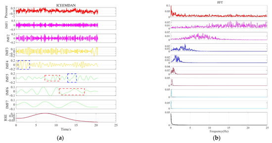
Figure 9.
IMF component and spectrogram of fluctuating pressure at the P2 measuring point: (a) ICEEMDAN; (b) FFT.
As depicted in Figure 9, the ICEEMDAN decomposition follows a descending order of frequency from the original signal decomposition to extract the modal components from low to high, culminating in the Res component, representing the trend term of the original signal. This process is characteristic of time-domain data for water flow fluctuating pressure, which exhibits weak non-stationarity and can be approximated as stationary.
Each modal component signal exhibited a more pronounced periodic pattern compared to the original signal. According to the theory of turbulence mechanics, the low-frequency segment of the signal corresponds to larger scales of vortices within turbulent flow, while the high-frequency segment corresponds to smaller scales of vortices. Consequently, the scales of vortex levels, represented by the transition from low-order to high-order components, gradually increase. Upon analyzing the IMF4 to IMF6 modal components, we observed a modal aliasing phenomenon resulting from the decomposition. Similar characteristic time-scale waveforms appeared in IMF4 and IMF5, as indicated by the blue dashed box, and this phenomenon persisted and was transmitted to higher orders, evident in the red dashed box in IMF5 and IMF6. It was shown that the blue characteristic waveforms in IMF4 and the red characteristic waveforms in IMF5 exhibited significant differences in time scales compared to the other positional characteristics, but both contained the same components found in IMF5. The presence of identical amplitude components at a specific frequency across the different component signals suggests the existence of vortices of comparable scales within vortex bodies of varying scale levels. The local amplitude of a single signal oscillates over time, representing the continuous variation in a specific vortex scale. This phenomenon reflects the development, mixing, and attenuation processes of vortices of various scales within the vortex structure. The diffusion and mixing of vortices across adjacent scales directly result in the pulsation of fluctuating pressure, which is of significant importance for understanding the mechanisms of turbulent mixing and energy transfer.
The IMF components derived from the decomposition of the measured fluctuating pressure signals in this paper using ICEEMDAN were subjected to Hilbert transformation to obtain their instantaneous frequencies and amplitudes. Subsequently, the instantaneous frequencies of all components, weighted by their amplitudes, were plotted on a time–frequency plane, resulting in a three-dimensional spectrogram depicting the signal’s time–frequency–amplitude (energy) characteristics, as shown in Figure 10. Additionally, Figure 10 illustrates the Hilbert spectrum of the fluctuating pressure signal measured at point P2 near the bottom edge of the gate under a small opening condition (e = 10%). The frequencies of all modal components of fluctuating pressure were observed to be within 25 Hz, with the high-energy region frequencies confined to 20 Hz or below. Overall, a distinct low-frequency characteristic was evident. As the decomposition order increased, the bandwidth of higher-order components narrowed significantly, and the amplitude of the Hilbert spectrum gradually decreased, along with a notable decline in Hilbert energy. Hence, the initial high-frequency components encompassed the majority of turbulent energy, albeit with low-frequency elements corresponding to the continuous intermixing and stochastic motion of vortices of varying scales within the turbulence. The instantaneous frequencies of individual components varied randomly over time, with Hilbert energy oscillating similarly. Sporadic abrupt changes were more pronounced in higher-order components. For instance, the primary frequency band of IMF1 was below 25 Hz (with a high-energy region below 20 Hz). However, the high-energy region of IMF2 rapidly narrowed to less than 10 Hz, and subsequently, the frequency band continued to narrow as the decomposition order increased. After IMF6, the bandwidth approached zero, and the amplitude of the Hilbert spectrum decreased to less than 5% of that of lower-order components. Nevertheless, the random oscillations in energy were significantly attenuated, reflecting the extremely weak non-stationary characteristics of the water flow pressure fluctuations.
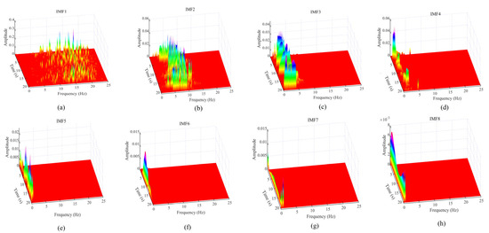
Figure 10.
Hilbert spectra of the components of eigenpoints. (a–h): IMF 1~8.
Based on the analysis in Figure 11, which integrated the results from other measurement points, the decomposition and Hilbert transformation of the fluctuating pressure signals on the gate panel revealed distinct frequency components. This process can be interpreted as decomposing the turbulent water flow into vortices of varying scales. The modal aliasing phenomenon of fluctuating pressure in each component further indicated the presence of multi-scale vortices within the turbulent vortex structure. The random diffusion and mixing of these vortices collectively contributed to the turbulence observed in the water flow.
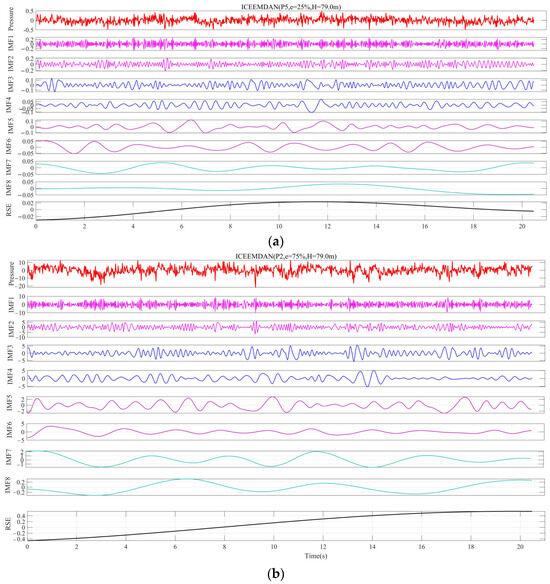
Figure 11.
ICEEMDAN decomposition results of fluctuating pressure at typical measurement points: (a) P5; (b) P2.
The preceding analysis demonstrates that the typical time series data of fluctuating water pressure exhibit weak non-stationarity, yet they can still be considered stationary to some extent. Furthermore, under specific operating conditions with e values of 10%, 25%, and 75%, the fluctuating pressure acting on the gate panel can be regarded as an ergodic stationary random process. The characteristic value of the ergodic stationary random process for fluctuating pressure acting on the gate can be obtained through random function theory and spectral analysis. This approach serves as a prerequisite for various other gate FIV analysis studies.
The presence of energy at a specific frequency in the Hilbert marginal spectrum indicates the potential occurrence of vibration at that frequency. The frequency corresponding to the maximum amplitude of the marginal spectrum represents the most likely vibration frequency, as well as the dominant frequency of primary interest in this study. This study utilized the Hilbert marginal spectrum to investigate the energy propagation patterns of fluctuating pressure signals. Figure 12 illustrates the Hilbert marginal spectrum at characteristic points along the surface of the radial gate panel.
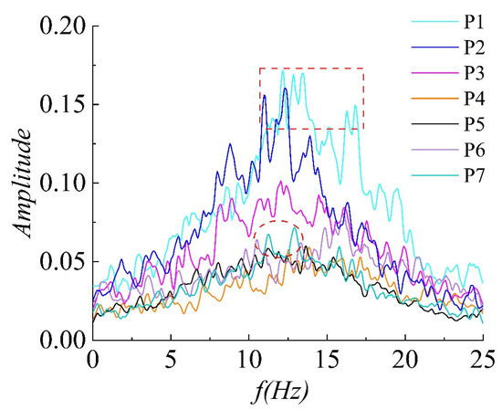
Figure 12.
The hilbert marginal spectrum of fluctuating pressure at measurement points on the gate panel at e = 25%.
The dominant frequencies at the seven measurement points on the gate panel were all below 20 Hz. Notably, the high-frequency components were more pronounced at P1 and P2 near the bottom edge, exhibiting significantly higher marginal spectrum amplitudes compared to the middle and upper sections of the gate. According to turbulence theory, low- and high-frequency components correspond to large- and small-scale vortices, respectively. Therefore, it can be inferred that the dominant large vortices in the turbulence gradually transform into small vortices here. In the experiments conducted in this study, the marginal spectrum energy of various characteristic points was primarily distributed below 20 Hz, with dominant frequencies ranging from approximately 10 to 15 Hz at each measurement point, indicating a prominent low-frequency characteristic of fluctuating pressure. The marginal spectrum, obtained by integrating the Hilbert spectrum of the fluctuating pressure signals on the panel along the time axis, visually reflected the dominant frequencies and marginal spectral energy at each measurement point, facilitating the interpretation of the spatial variation of turbulence energy on the gate panel.
4.2. The Pressure Prediction on the Gate Panel
The data-driven method involves utilizing patterns and relationships within data to construct predictive and decision-making models. To study the effects of hydrodynamic loads, a hydrodynamic predictive analysis model can be developed. For predicting and analyzing the time-series data pertaining to hydrodynamic loads, an LSTM model can accurately reflect the trends and patterns of hydrodynamic load changes over time.
4.2.1. Parameter Settings
Prior to training, data normalization and sample partitioning are necessary. To evaluate the model’s adaptability and verify its predictive performance, 70% of the sample data was selected as the training set for model training, while the remaining 30% was designated as the validation set to assess the model’s predictive capabilities.
The LSTM parameters were set as follows: a learning rate of 0.01, 100 training epochs, and a two-hidden-layer structure with 50 neurons in each hidden layer. After completing these settings, the data were input to generate the experimental results of the LSTM model.
The optimal parameters for model training were established as follows: a sparrow group size of 10, a discoverer ratio of 20%, an alarm threshold of 0.8, a learning rate range of [0.001, 0.01], an iteration range of [10, 100], a number of hidden layer neurons ranging from 1 to 100, and 25 training epochs. During the training process, the SSA optimization algorithm was employed to continuously adjust the number of neurons in the two hidden layers, the number of iterations, and the learning rate of LSTM. Training was terminated when no further improvement in fitness was observed over several consecutive iterations. The determination of optimization parameters is shown in Figure 13. When the number of neurons in the two hidden layers was 53 and 29, respectively, the number of iterations was 80, and the learning rate was 0.0062; the model achieved optimal performance.
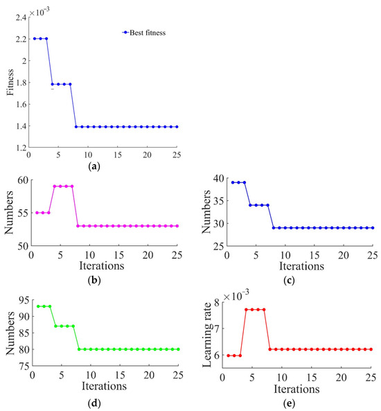
Figure 13.
Determination of optimization parameters. (a) Fitness curve; (b) first hidden node optimization; (c) second hidden node optimization; (d) iterative optimization; (e) learning rate optimization.
4.2.2. Prediction and Comparative Analysis
To better characterize the accuracy and generalization of the model’s output, the model was evaluated using the EMAP (mean absolute percentage error), EMS (mean square error), ERMS (root mean square error), EMA (mean absolute error), and R2 (goodness fit) [33]. The calculation formulas for these metrics are as follows:
where N represents the total number of samples, Pk denotes the predicted value of the kth sample, Ok indicates the observed value of the k-th sample, and represents the average of all observed values for the samples.
It is generally believed that a higher R2 value, accompanied by lower values of EMAP, ERMS, EMA, and EMS, indicates superior model performance. A comparative analysis of the prediction processes of the three models is presented in Figure 14, while scatter plots comparing the actual measured values with the predicted values are depicted in Figure 15.
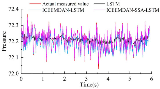
Figure 14.
Comparison of the prediction process of the three models.
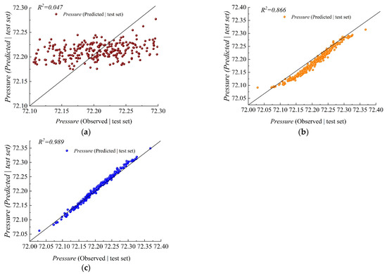
Figure 15.
Scatter of measured and predicted values for the three models. (a) LSTM prediction results; (b) ICEEMDAN-LSTM prediction results; (c) ICEEMDAN-SSA-LSTM prediction results.
Figure 14 illustrates that the LSTM model exhibits a notable discrepancy from the actual values, resulting in inferior prediction performance. In contrast, both the ICEEMDAN-SSA-LSTM and ICEEMDAN-LSTM models demonstrate a higher degree of overlap with the measured values, indicating superior predictive effects. However, no discernible differences are observed between the two models. Furthermore, an analysis of the scatter plot in Figure 15 and the radar chart in Figure 16 reveals that the ICEEMDAN-SSA-LSTM model outperformed the ICEEMDAN-LSTM model in terms of peak prediction accuracy during the validation period, while the LSTM model exhibited lower peak prediction accuracy.
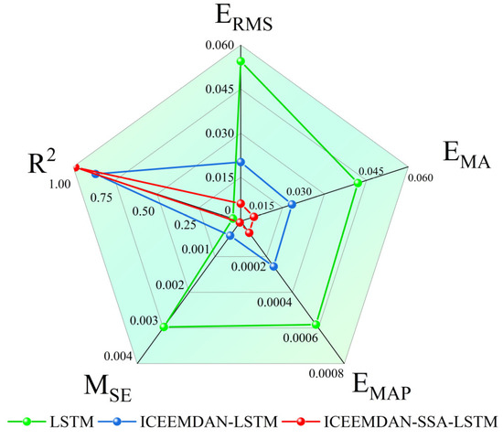
Figure 16.
Predictive testing indicators.
5. Discussion
According to turbulence theory, the low- and high-frequency components correspond to large- and small-scale vortices, suggesting that the large vortices, the main components of turbulence, gradually transform into smaller ones. The analysis above indicates that the local amplitude in a single signal oscillates over time, reflecting changes in vortex scale levels and the development, mixing, and attenuation processes of vortex structures at different scales. Vortices at neighboring scales constantly undergo diffusion and mixing, leading to fluctuations in fluctuating pressure.
In conclusion, the unsatisfactory prediction outcomes of the LSTM model can be attributed to its “black box” nature. The LSTM model fails to capture the underlying physical mechanisms of fluctuating pressure on the gate panel as it relies solely on a single time series. In scenarios involving high velocity and turbulence, the formation mechanism of fluctuating pressure in turbulent areas becomes more intricate, leading to limited prediction accuracy with single time series models. In some cases, the predicted results may not align with actual demands. The ICEEMDAN-SSA-LSTM model, on the other hand, demonstrates superior prediction accuracy during both training and validation periods. ICEEMDAN decomposition effectively reduces noise in the original fluctuating pressure sequence while extracting complex and informative data from vortices at various scales. This approach offers a more nuanced understanding of the intrinsic mechanism behind fluctuating pressure formation. Additionally, SSA optimizes LSTM model parameters, streamlining parameter selection and enhancing efficiency.
Therefore, the ICEEMDAN-SSA-LSTM model proposed in this paper significantly improves signal prediction accuracy, making it suitable for fluctuating pressure prediction on gate panels.
6. Conclusions
This paper presents the results of hydrodynamic tests conducted on a submerged radial gate at a high-head flood discharge outlet. Initially, a hydraulic model test with a scale ratio of 1:25 was conducted to study the fluctuating pressure distribution on the gate panel under different opening conditions. Then, using the ICEEMDAN-HHT theory, the characteristics and causes of the fluctuating pressure on the panel were systematically analyzed. Furthermore, a deep learning method, ICEEMDAN-SSA-LSTM, was employed to predict the fluctuating pressure on the gate panel. The following conclusions were drawn:
- (1)
- The load acting on the gate panel is primarily time averaged, with the RMS of fluctuating pressure constituting less than 10% of the time-average pressure. The RMS of fluctuating pressure near the bottom is significantly higher than that in the middle and top of the gate, while the time-average pressure in the middle is higher than that at the bottom and top of the gate. It is noteworthy that there is a notable disparity between the distribution of fluctuating pressure and hydrostatic pressure at the gate.
- (2)
- Decomposing the fluctuating pressure signal of the gate panel reveals that the time-domain data of water fluctuating pressure are weakly non-stationary but can be considered stationary to some extent. Based on this, applying the improved Hilbert transform to each IMF component yields different frequency-band components, which can be interpreted as a decomposition of turbulent water flow into vortices at various scales. Moreover, the modal aliasing of fluctuating pressures of each component indicates that the turbulent vortex structure contains multi-scale vortices, whose random diffusion and mixing collectively contribute to the turbulent behavior of the flow.
- (3)
- A fluctuating pressure prediction method based on ICEEMDAN-SSA-LSTM was proposed to improve the accuracy of the gate panel fluctuating pressure signal compared to the LSTM and ICEEMDAN-LSTM prediction methods. This method can provide technical support for subsequent gate vibration signal detection and fault diagnosis.
Author Contributions
Conceptualization, X.L. and Y.L. (Yakun Liu); methodology, X.L., S.T. and W.B.; software, X.L. and Y.L.(Yangliang Lu); validation, X.L., W.B. and X.Z.; formal analysis, W.B. and X.Z.; investigation, W.B.; resources, Y.L. (Yakun Liu) and S.T.; data curation, X.L.; writing—original draft preparation, X.L.; writing—review and editing, Y.L. (Yakun Liu); visualization, Y.L. (Yangliang Lu); supervision, S.T. and Y.L. (Yakun Liu); project administration, S.T. and Y.L. (Yakun Liu); funding acquisition, S.T. and Y.L. (Yakun Liu). All authors have read and agreed to the published version of the manuscript.
Funding
This research was funded by Science and Technology Projects of CHINA HUANENG GROUP (grant No. HNKJ22-H108), Science and Technology Projects of China Power Construction Corporation Limited (grant No. DJ-ZDXM-2021-03), and the National Natural Science Foundation of China (grant No. 52179060).
Informed Consent Statement
Not applicable.
Data Availability Statement
The raw data supporting the conclusions of this article will be made available by the authors on request.
Conflicts of Interest
Authors Xiudi Lu, Shoulin Tan and Wei Bao were employed by the company Power China Guiyang Engineering Corporation Limited. The remaining authors declare that the re-search was conducted in the absence of any commercial or financial relationships that could be construed as a potential conflict of interest.
References
- Kanthakasikam, R.; Charatpangoon, B.; Hansapinyo, C.; Buachart, C.; Kiyono, J. Seismic Safety Analysis of Dam Appurtenant Structures in Northern Thailand. KSCE J. Civ. Eng. 2024, 28, 2885–2896. [Google Scholar] [CrossRef]
- Faridmehr, I.; Farokhi Nejad, A.; Baghban, M.H.; Ghorbani, R. Numerical and Physical Analysis on the Response of a Dam’s Radial Gate to Extreme Loading Performance. Water 2020, 12, 2425. [Google Scholar] [CrossRef]
- Wang, Z.; Zhang, X.; Liu, J. Advances and developing trends in research of large hydraulic steel gates. J. Hydroelectr. Eng. 2017, 36, 1–18. (In Chinese) [Google Scholar] [CrossRef]
- Lu, Y.; Liu, Y.; Zhang, D.; Cao, Z.; Fu, X. Chaotic Characteristic Analysis of Spillway Radial Gate Vibration under Discharge Excitation. Appl. Sci. 2023, 14, 99. [Google Scholar] [CrossRef]
- Xu, C.; Liu, J.; Zhao, C.; Liu, F.; Wang, Z. Dynamic failures of water controlling radial gates of hydro-power plants: Advancements and future perspectives. Eng. Fail. Anal. 2023, 148, 107168. [Google Scholar] [CrossRef]
- Xu, C.; Wang, Z. New insights into dynamic instability regions of spillway radial gate owing to fluid-induced parametric oscillation. Nonlinear Dyn. 2022, 111, 4053–4070. [Google Scholar] [CrossRef]
- Wang, C.; Hou, D.; Li, L.; Xia, Y. Study of shape design of the aerator with sudden lateral enlargement and bottom drop behind high-head radial gate and its engineering applicaton. J. Hydroelectr. Eng. 2012, 35, 107–113. (In Chinese) [Google Scholar]
- Chen, J.; Zhou, G.G.D.; Chen, X.; Zhang, J.; Li, S. Characteristics of aeration in the flow downstream of a radial gate with a sudden fall-expansion aerator in a discharge tunnel. Water Supply 2018, 18, 790–798. [Google Scholar] [CrossRef]
- Lei, G.; Huang, H.; Fan, X.; Su, J.; Wang, Q.; Wang, X.; Peng, K.; Zhang, J. Influence of the transition section shape on the cavitation characteristics at the bottom outlet. Water Supply 2023, 23, 3061–3077. [Google Scholar] [CrossRef]
- Jamali, T.; Manafpour, M.; Ebrahimnezhadian, H. Evolution of pressure and cavitation in transition region walls for supercritical flow. J. Water Supply Res. Technol. Aqua 2023, 72, 62–82. [Google Scholar] [CrossRef]
- Li, J.; Wang, C.; Wang, Z.; Ren, K.; Zhang, Y.; Xu, C.; Li, D. Numerical Analysis of Flow-Induced Vibration of Deep-Hole Plane Steel Gate in Partial Opening Operation. Sustainability 2022, 14, 13616. [Google Scholar] [CrossRef]
- Yan, G.; Yan, S.; Fan, B.; Luo, S.; Chen, F.; Wang, Z.; Chan, Q.; Teng, S. Study of Flow-induced Vibration for the High-head and Large Di mension Gate. J. Hydroelectr. Eng. 2001, 4, 65–75. (In Chinese) [Google Scholar]
- Lian, J.; Chen, L.; Ma, B.; Liang, C. Analysis of the Cause and Mechanism of Hydraulic Gate Vibration during Flood Discharging from the Perspective of Structural Dynamics. Appl. Sci. 2020, 10, 629. [Google Scholar] [CrossRef]
- Zhang, W.; Yan, G.; Chen, F.; Dong, J. Static and dynamic characteristics of high pressure radial gate and its flow-induced vibration. Hydro-Sci. Eng. 2016, 2, 111–119. [Google Scholar] [CrossRef]
- Lee, S.O.; Seong, H.; Kang, J.W. Flow-induced vibration of a radial gate at various opening heights. Eng. Appl. Comput. Fluid Mech. 2018, 12, 567–583. [Google Scholar] [CrossRef]
- Daneshmand, F.; Adamowski, J.; Liaghat, T. Bottom outlet dam flow: Physical and numerical modelling. Proc. Inst. Civ. Eng. Water Manag. 2014, 167, 176–184. [Google Scholar] [CrossRef]
- Wang, Y.; Tian, T.; Xu, G.; Liu, F. Calculation method of panel hydrodynamic pressure of radial gate. J. Huazhong Univ. Sci. Tech. (Nat. Sci. Ed.) 2021, 49, 102–107. (In Chinese) [Google Scholar] [CrossRef]
- Zhang, B.; Jing, X. Theoretical analysis and simulation calculation of hydrodynamic pressure pulsation effect and flow induced vibration response of radial gate structure. Sci. Rep. 2022, 12, 21932. [Google Scholar] [CrossRef]
- Hu, G.; Kwok, K.C.S. Predicting wind pressures around circular cylinders using machine learning techniques. J. Wind. Eng. Ind. Aerodyn. 2020, 198, 104099. [Google Scholar] [CrossRef]
- Sudharsun, G.; Warrior, H.V. Enhancing turbulence modeling: Machine learning for pressure-strain correlation and uncertainty quantification in the Reynolds stress model. Phys. Fluids 2023, 35, 125112. [Google Scholar] [CrossRef]
- Zhao, S.X.; Ma, L.S.; Xu, L.Y.; Liu, M.N.; Chen, X.L. A Study of Fault Signal Noise Reduction Based on Improved CEEMDAN-SVD. Appl. Sci. 2023, 13, 10713. [Google Scholar] [CrossRef]
- Hou, G.; Xu, K.; Lian, J.J.; Cai, O. Vibration prediction of offshore wind turbines based on long short-term memory network. Ships Offshore Struct. 2023, 1–11. [Google Scholar] [CrossRef]
- Agga, A.; Abbou, A.; Labbadi, M.; El Houm, Y.; Ali, I.H.O. CNN-LSTM: An efficient hybrid deep learning architecture for predicting short-term photovoltaic power production. Electr. Power Syst. Res. 2022, 208, 107908. [Google Scholar] [CrossRef]
- Colominas, M.A.; Schlotthauer, G.; Torres, M.E. Improved complete ensemble EMD: A suitable tool for biomedical signal processing. Biomed. Signal Process. Control 2014, 14, 19–29. [Google Scholar] [CrossRef]
- Huang, N.E.; Shen, Z.; Long, S.R.; Wu, M.L.C.; Shih, H.H.; Zheng, Q.N.; Yen, N.C.; Tung, C.C.; Liu, H.H. The empirical mode decomposition and the Hilbert spectrum for nonlinear and non-stationary time series analysis. Proc. R. Soc. A-Math. Phys. Eng. Sci. 1998, 454, 903–995. [Google Scholar] [CrossRef]
- Jia, W.; Diao, M.; Jiang, L.; Huang, G. Fluctuating Characteristics of the Stilling Basin with a Negative Step Based on Hilbert-Huang Transform. Water 2021, 13, 2673. [Google Scholar] [CrossRef]
- Xue, J.; Shen, B. A novel swarm intelligence optimization approach: Sparrow search algorithm. Syst. Sci. Control Eng. 2020, 8, 22–34. [Google Scholar] [CrossRef]
- Hochreiter, S.; Schmidhuber, J. Long short-term memory. Neural Comput. 1997, 9, 1735–1780. [Google Scholar] [CrossRef]
- Mishra, M.; Byomakesha Dash, P.; Nayak, J.; Naik, B.; Kumar Swain, S. Deep learning and wavelet transform integrated approach for short-term solar PV power prediction. Measurement 2020, 166, 108250. [Google Scholar] [CrossRef]
- Pfister, M.; Hager, W.H. Chute Aerators. I: Air Transport Characteristics. J. Hydraul. Eng. 2010, 136, 352–359. [Google Scholar] [CrossRef]
- Gioffrè, M.; Gusella, V. Damage accumulation in glass plates. J. Eng. Mech. 2002, 128, 801–805. [Google Scholar] [CrossRef]
- Lu, Y.; Yin, J.; Yang, Z.; Wei, K.; Liu, Z. Numerical Study of Fluctuating Pressure on Stilling Basin Slab with Sudden Lateral Enlargement and Bottom Drop. Water 2021, 13, 238. [Google Scholar] [CrossRef]
- Khan, Z.A.; Hussain, T.; Ullah, A.; Rho, S.; Lee, M.; Baik, S.W. Towards Efficient Electricity Forecasting in Residential and Commercial Buildings: A Novel Hybrid CNN with a LSTM-AE based Framework. Sensors 2020, 20, 1399. [Google Scholar] [CrossRef] [PubMed]
Disclaimer/Publisher’s Note: The statements, opinions and data contained in all publications are solely those of the individual author(s) and contributor(s) and not of MDPI and/or the editor(s). MDPI and/or the editor(s) disclaim responsibility for any injury to people or property resulting from any ideas, methods, instructions or products referred to in the content. |
© 2024 by the authors. Licensee MDPI, Basel, Switzerland. This article is an open access article distributed under the terms and conditions of the Creative Commons Attribution (CC BY) license (https://creativecommons.org/licenses/by/4.0/).