

Sequence Deep Learning for Seismic Ground Response Modeling: 1D-CNN, LSTM, and Transformer Approach


Abstract
1. Introduction
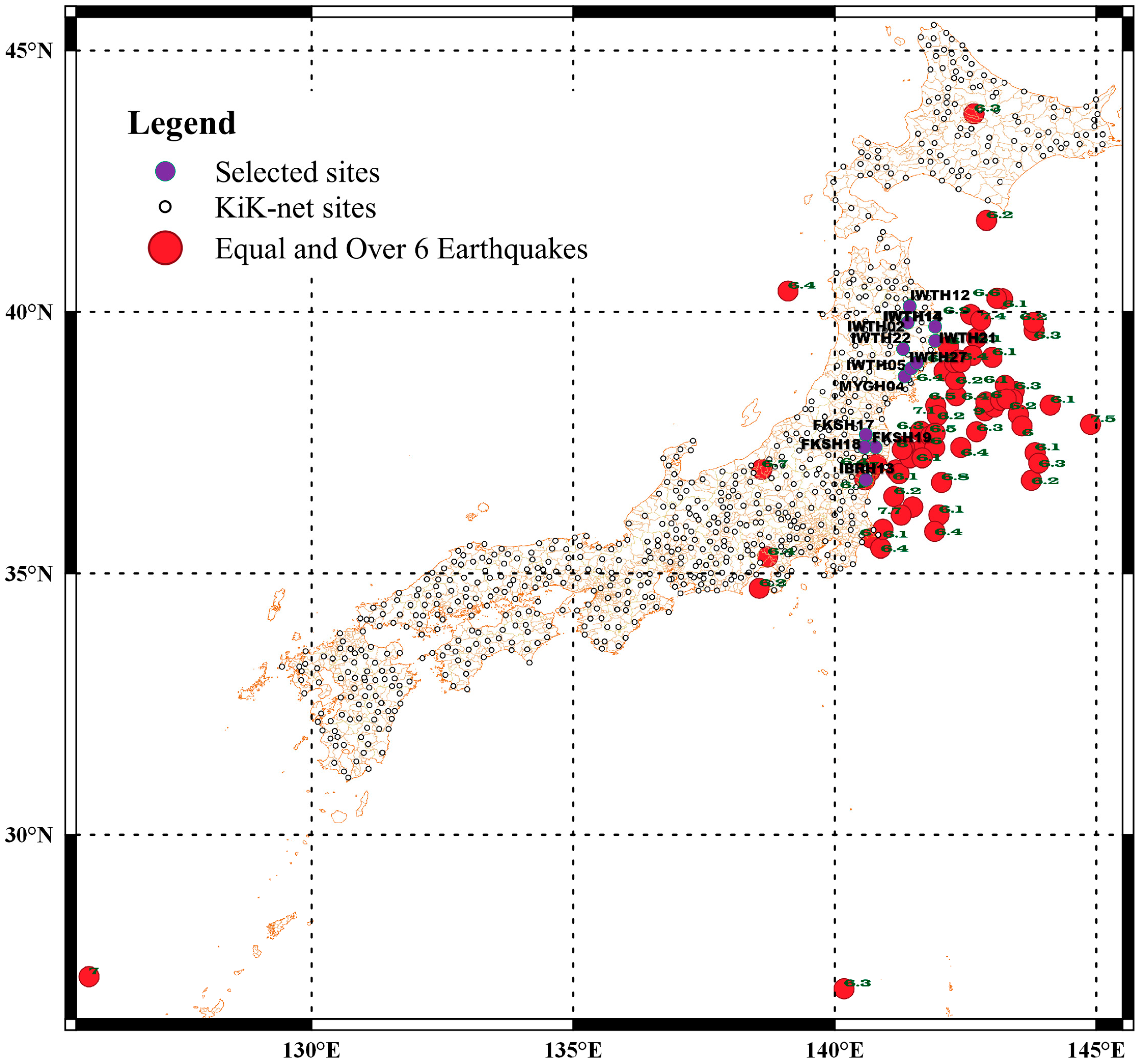
2. Earthquake Data
3. Prediction Models
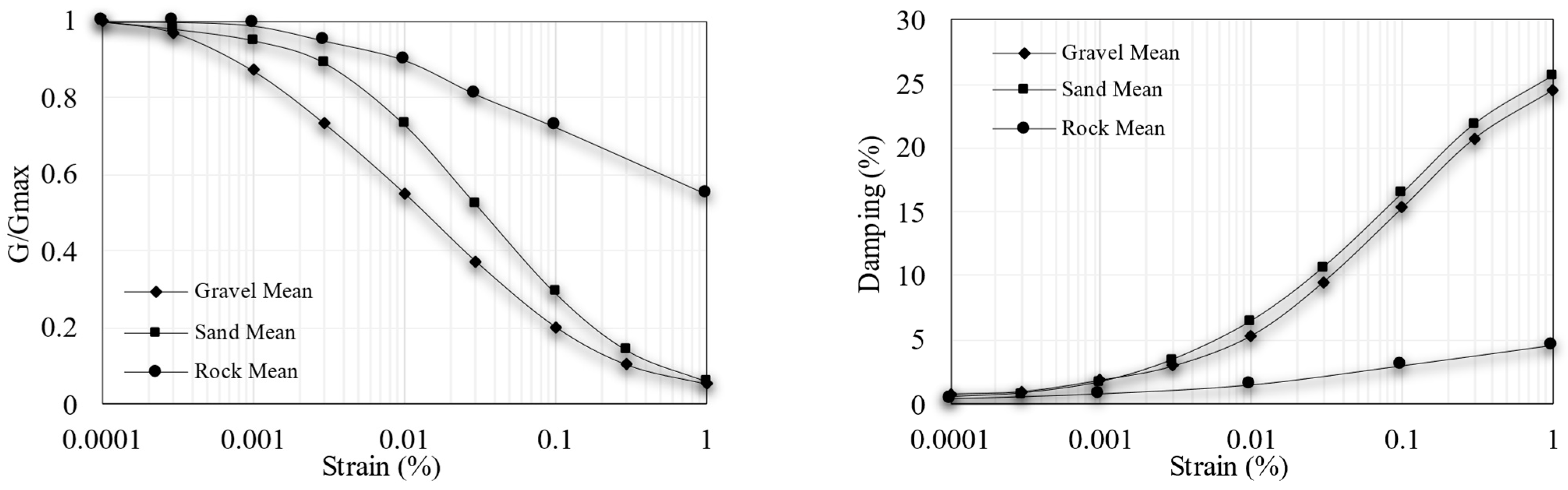
3.1. Physics-Based Model
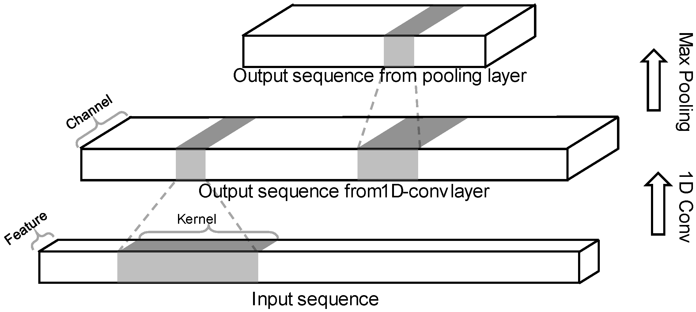
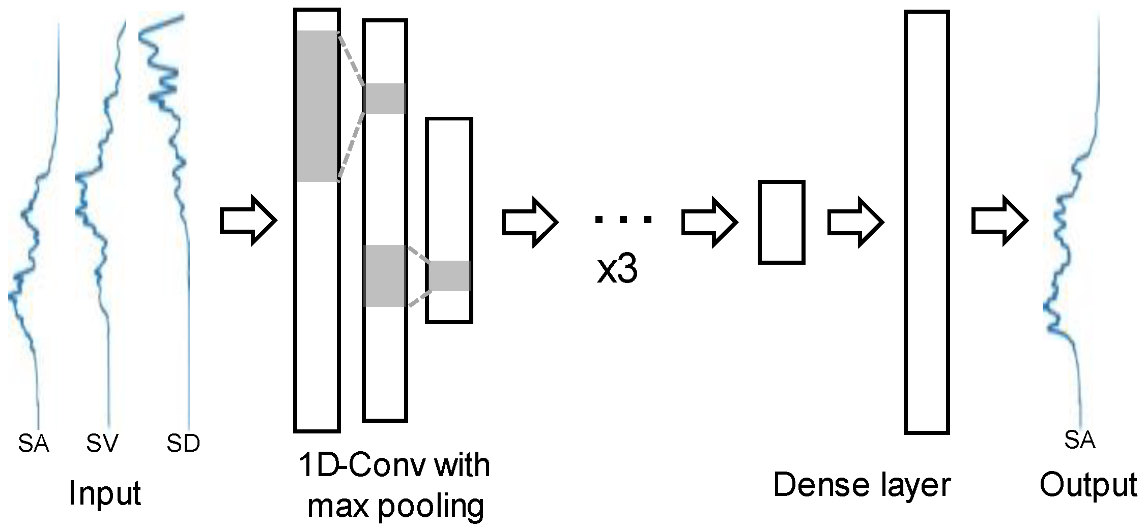
3.2. One-Dimensional Convolutional Neural Network (CNN)-Based Model
3.2.1. Overview
3.2.2. Model Architecture
3.3. Long Short-Term Memory (LSTM) Networks-Based Model
3.3.1. Overview
3.3.2. Model Architecture
3.4. Transformer-Based Model
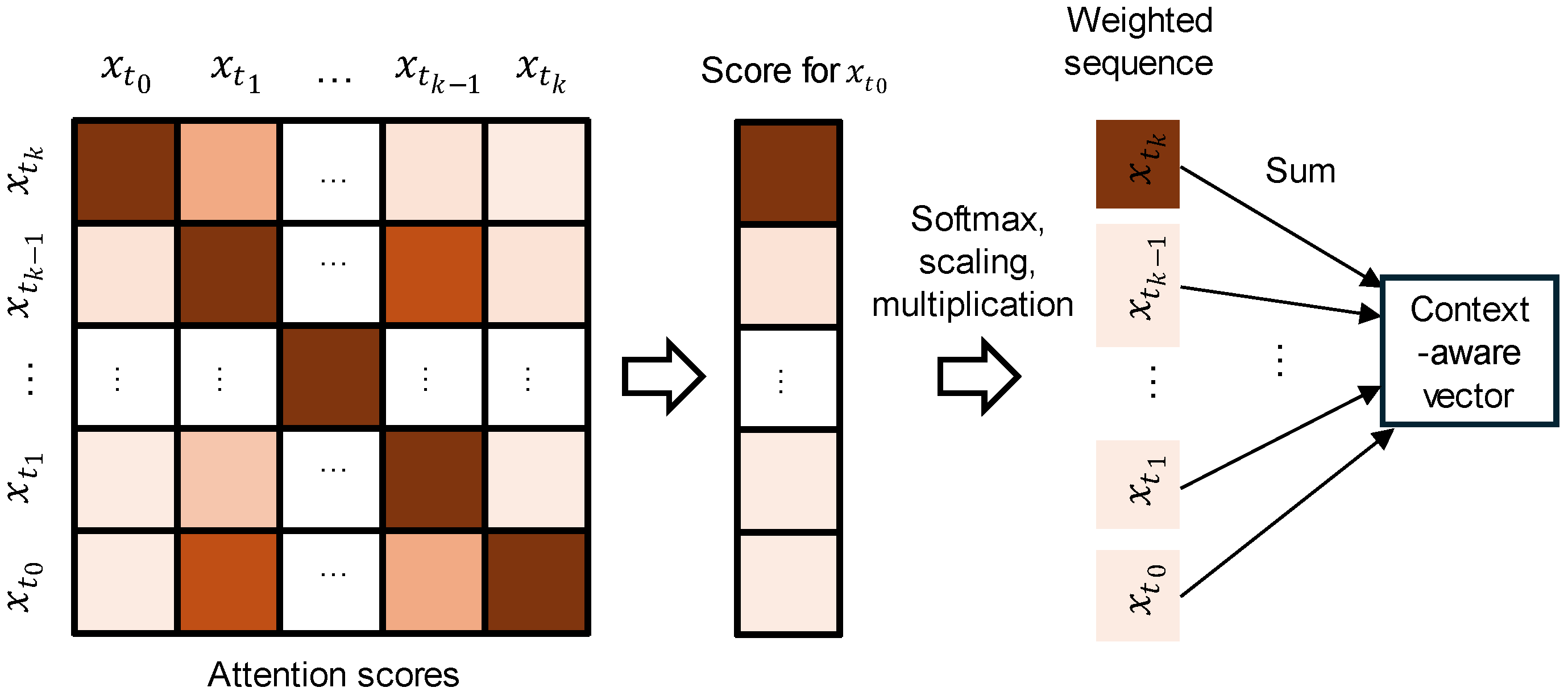
3.4.1. Overview
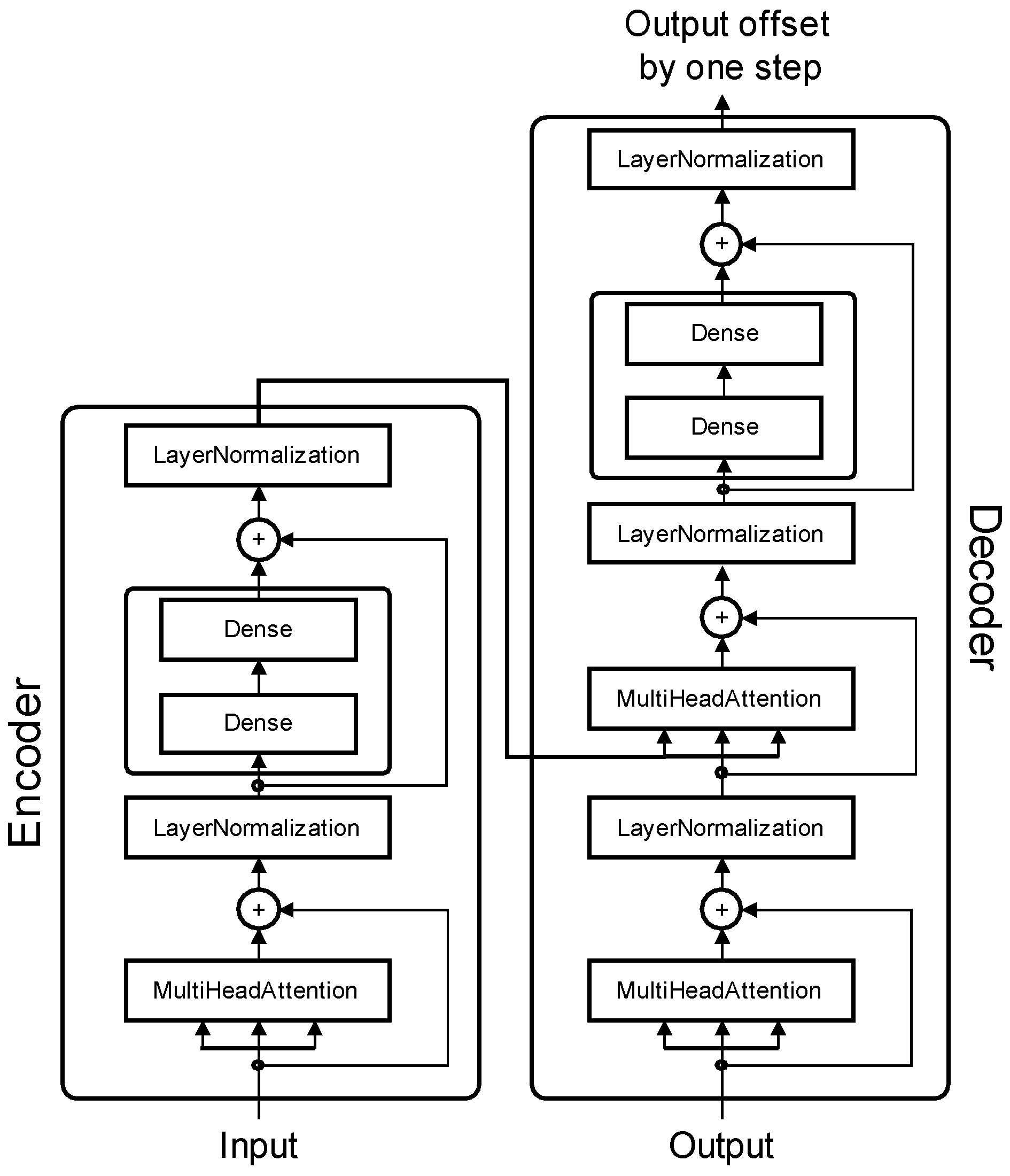
3.4.2. Model Architecture
4. Training
5. Results and Discussion
5.1. Prediction Performance
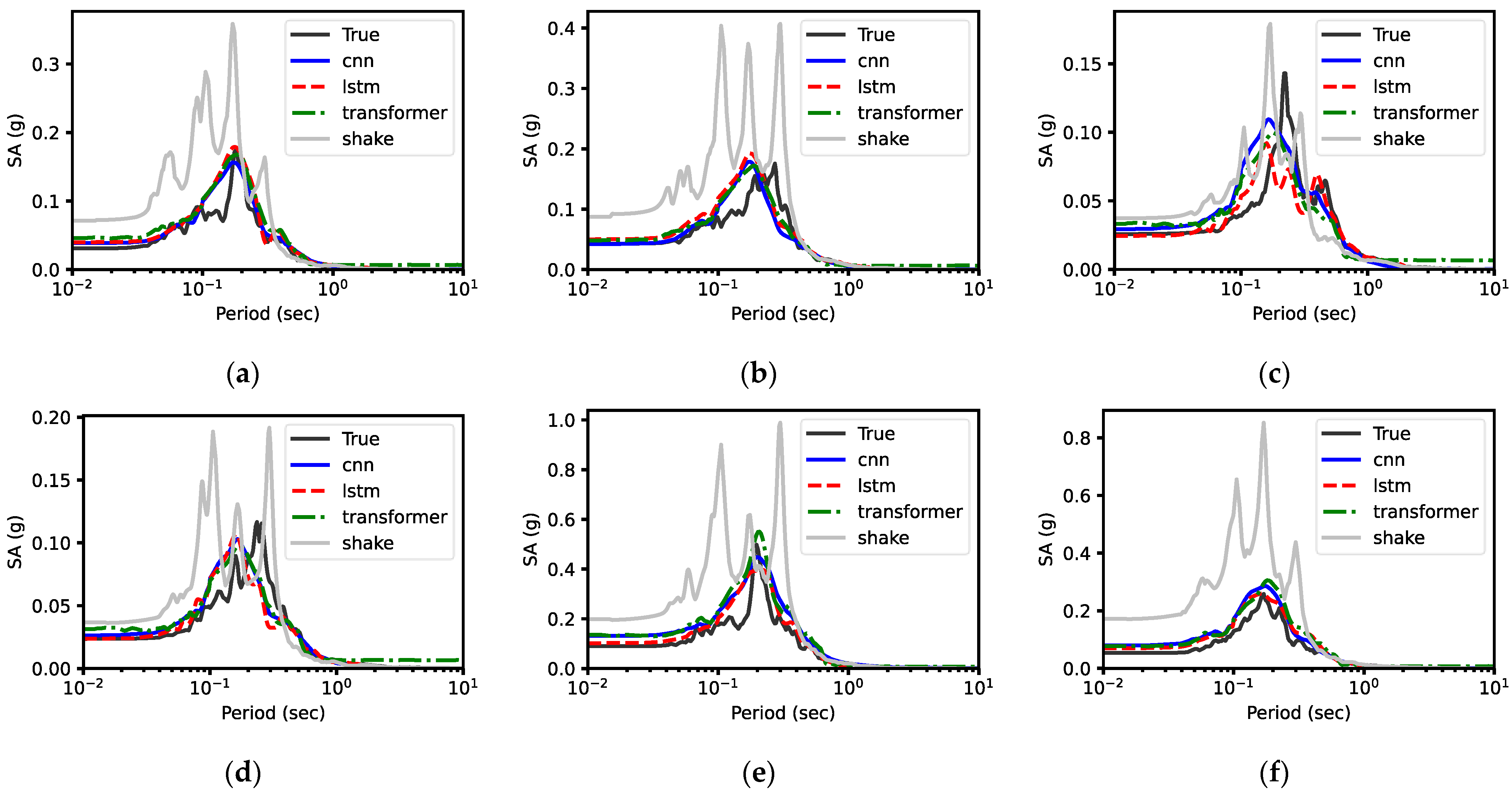
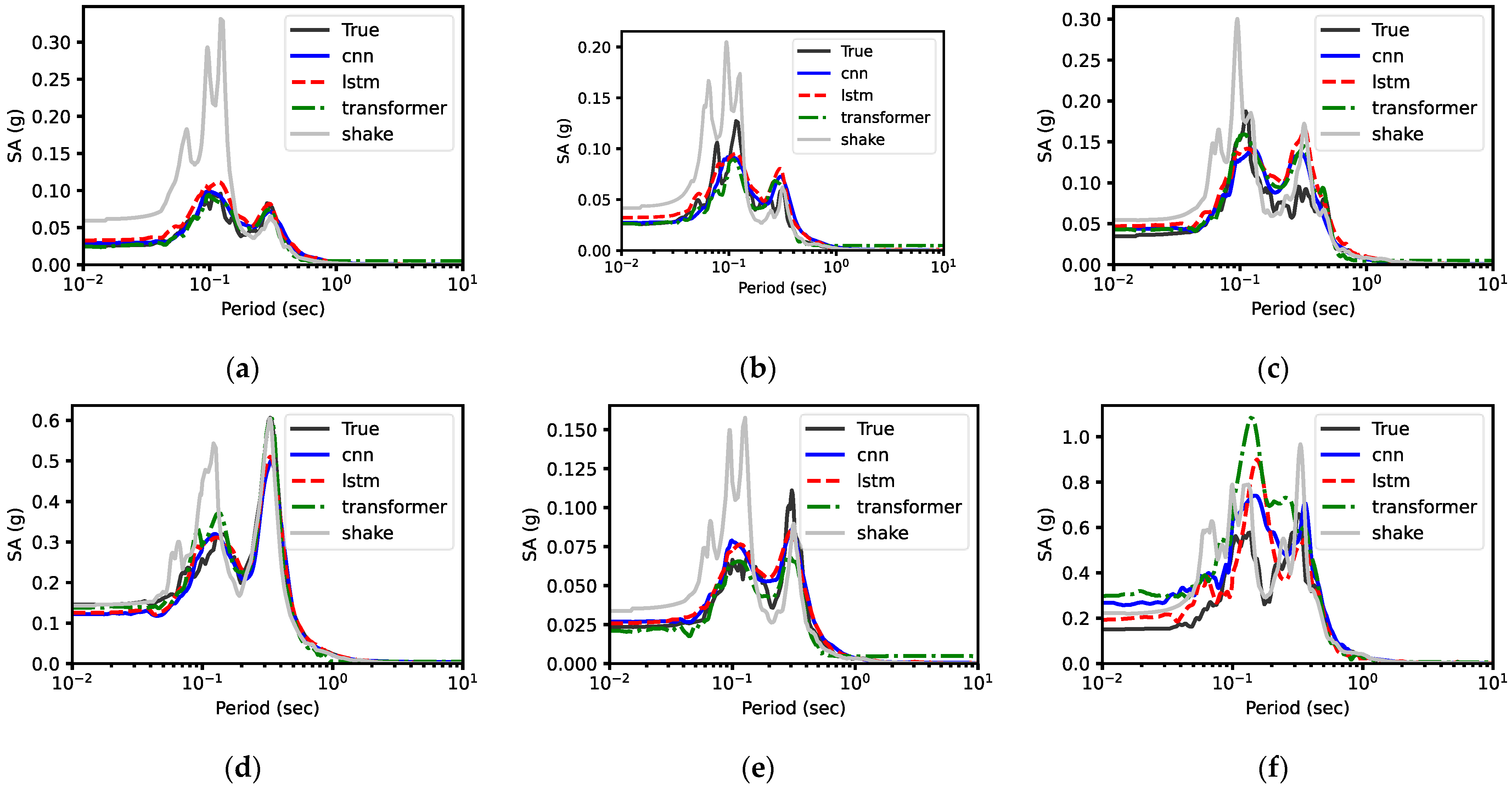
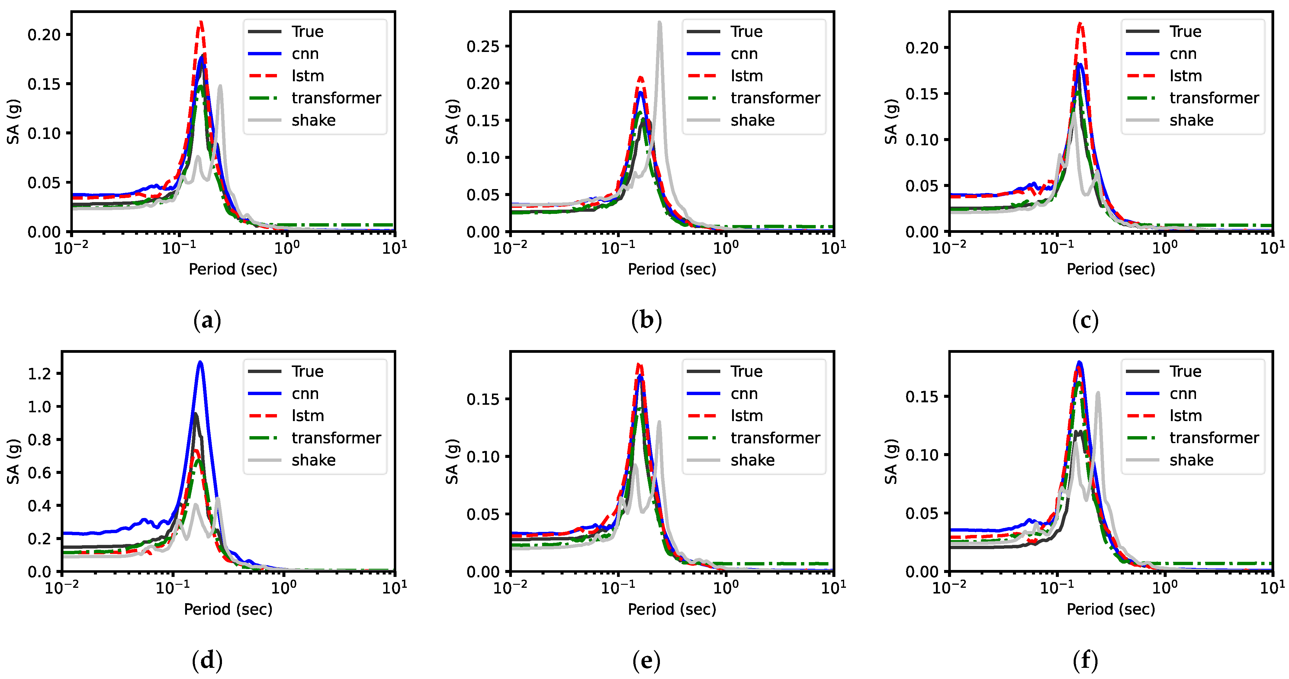
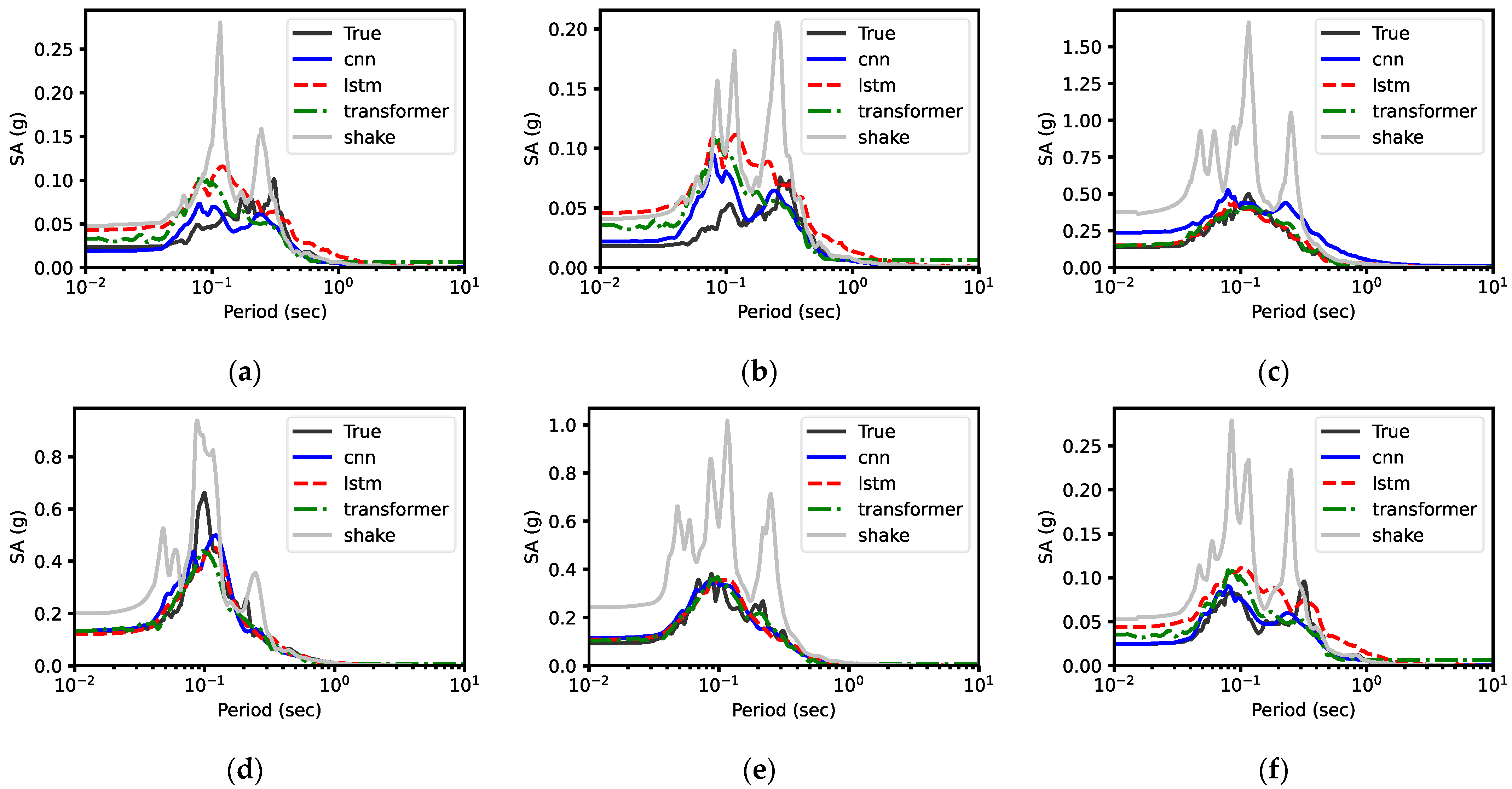
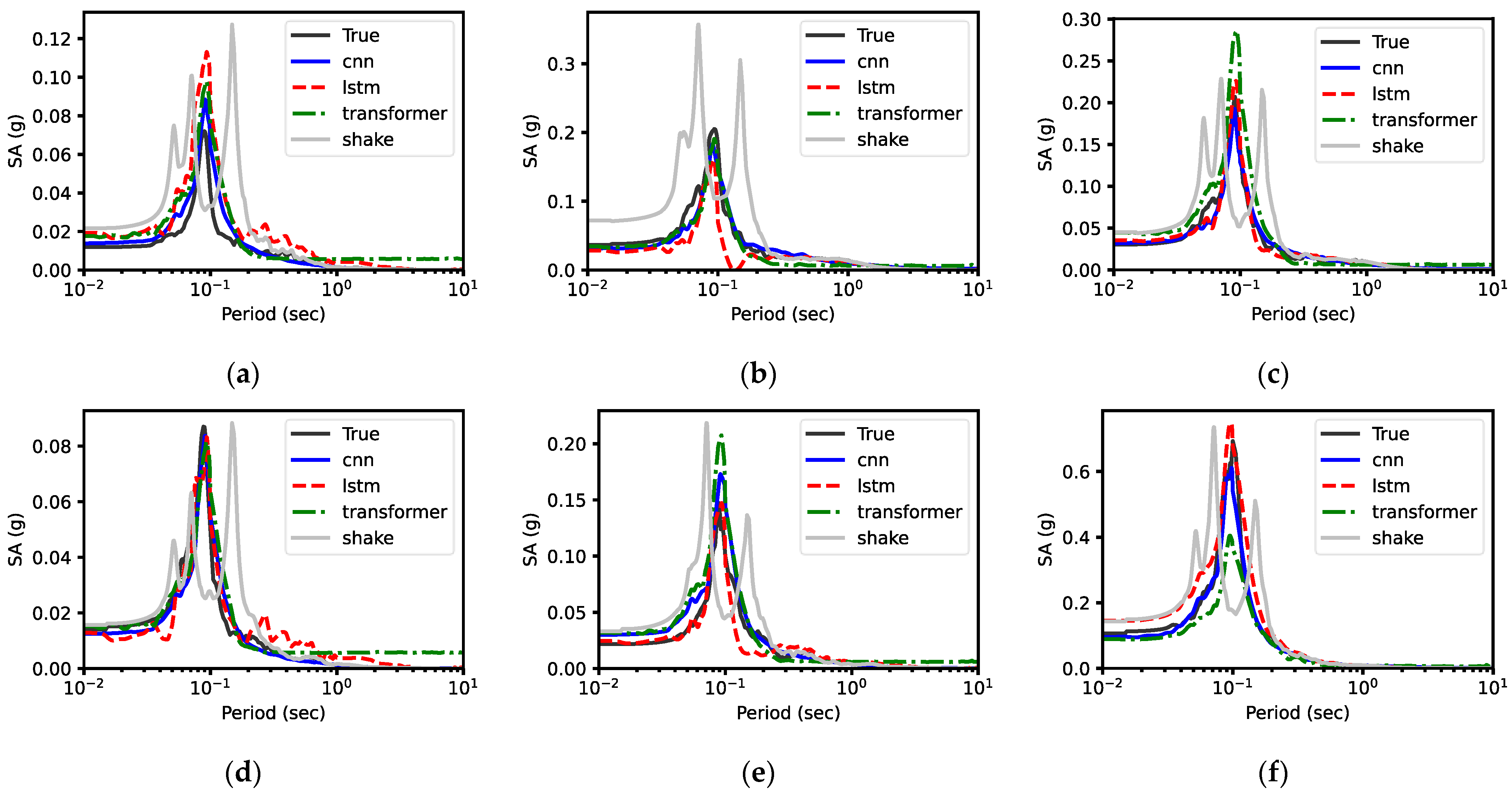
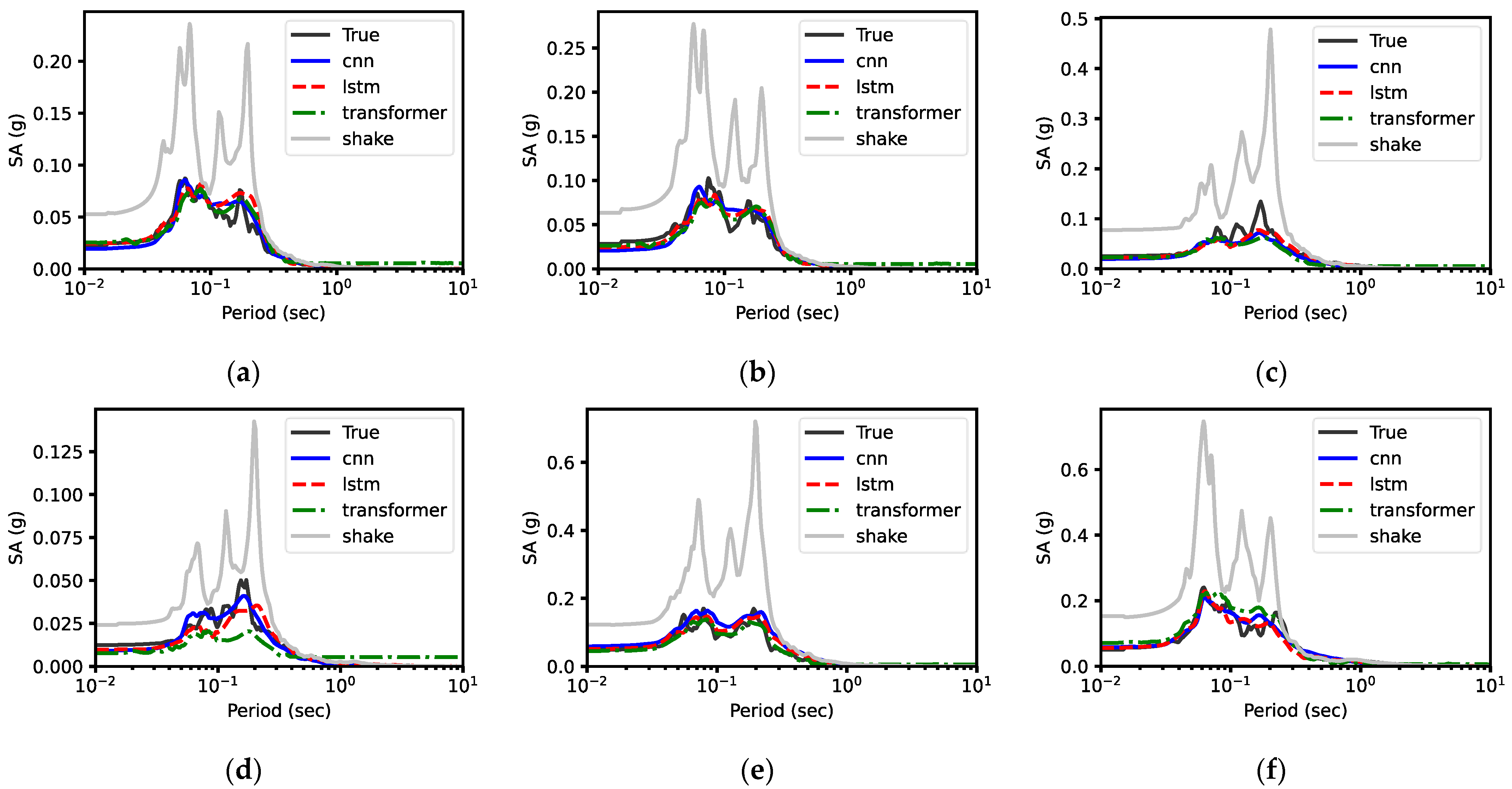
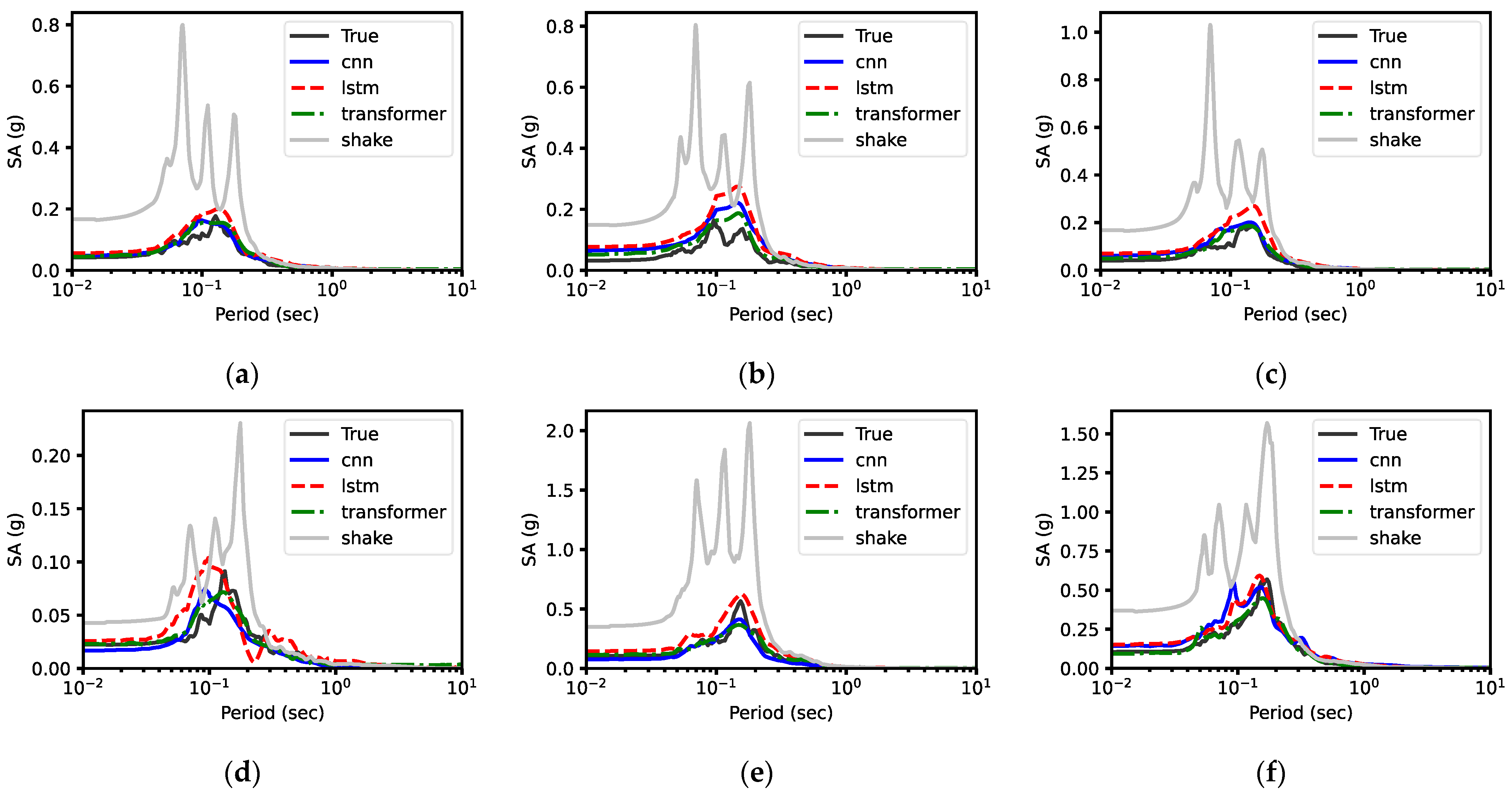
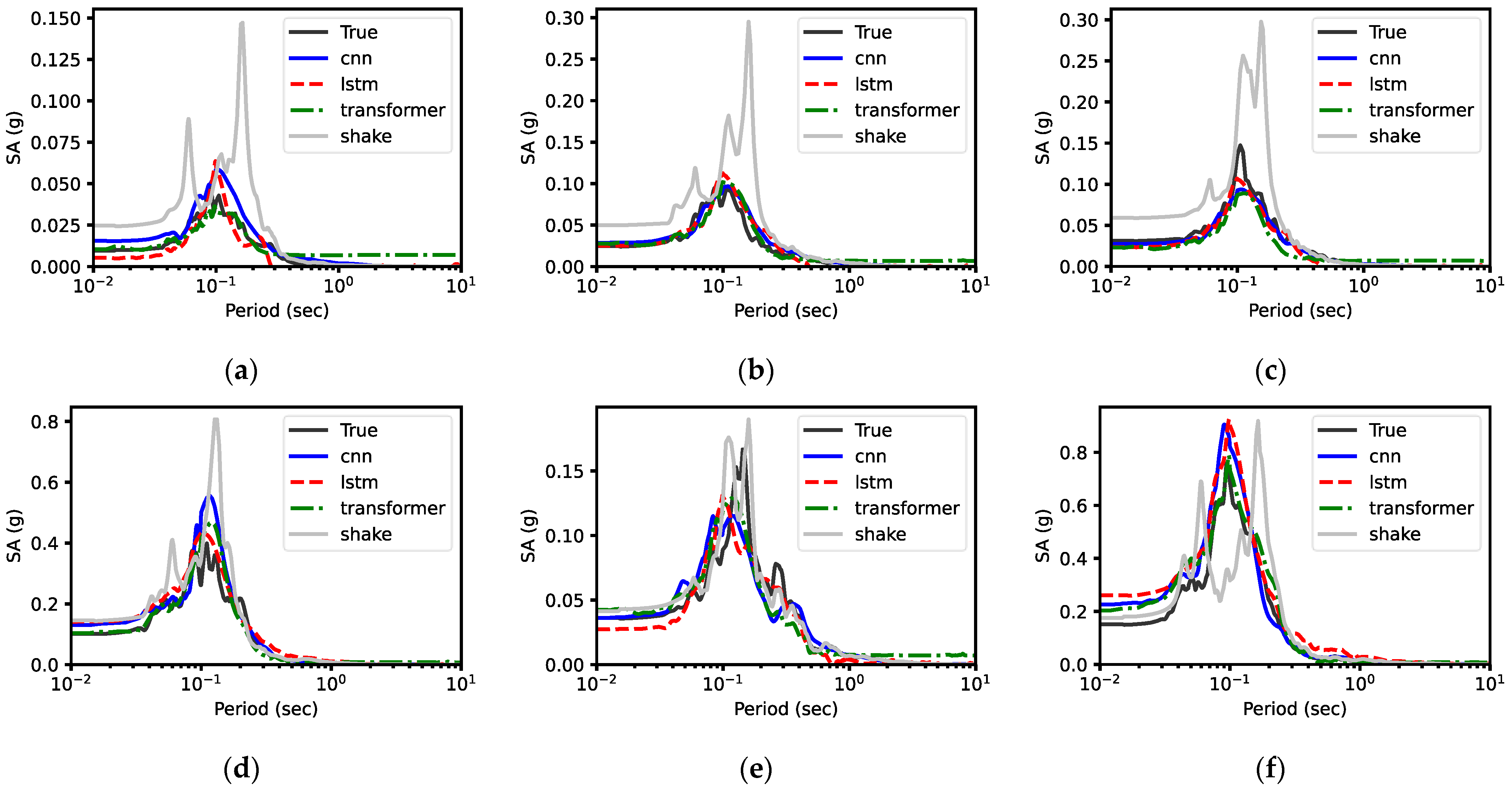
5.1.1. Response Spectra
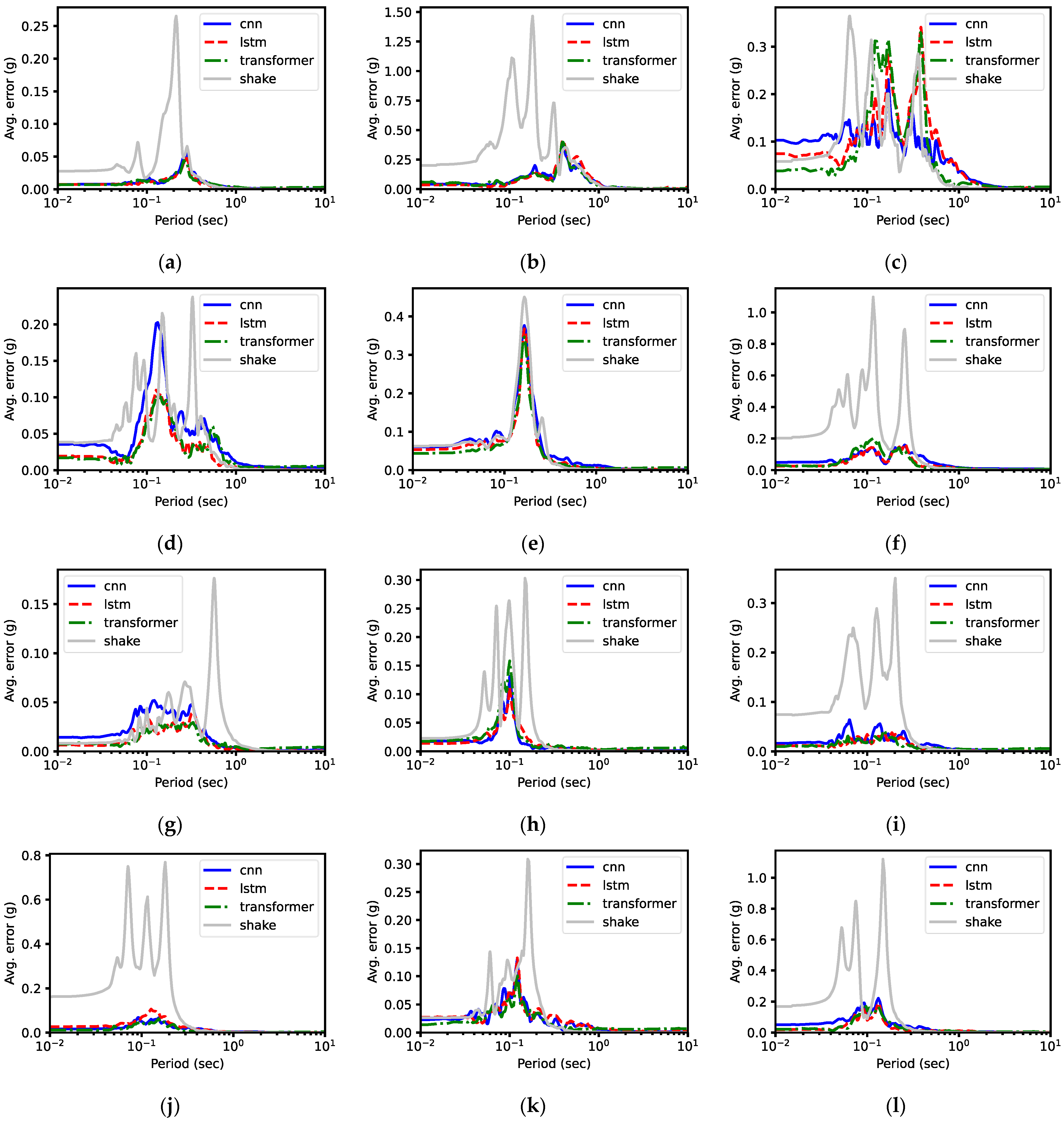
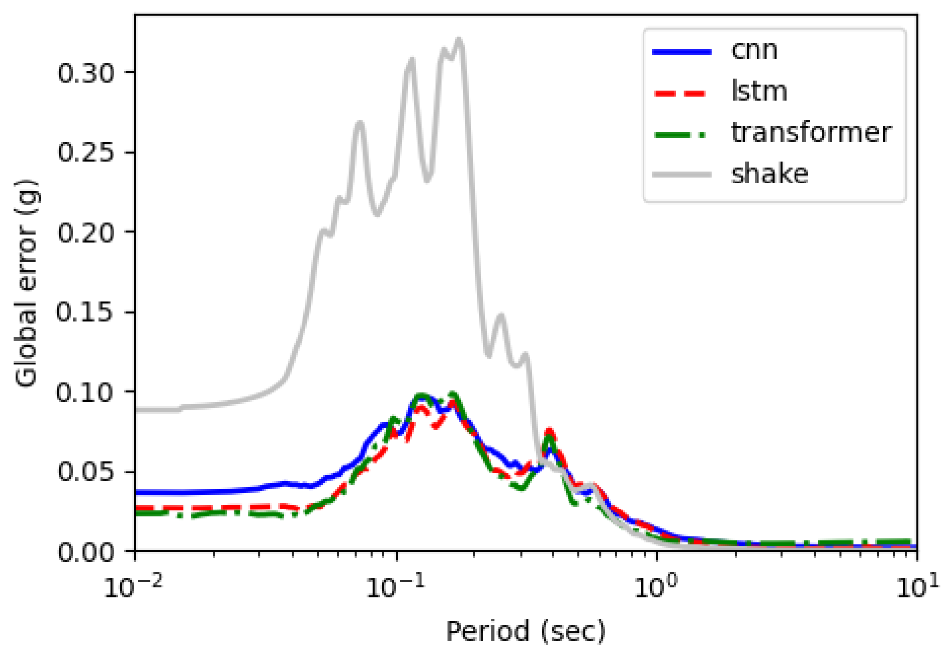
5.1.2. Prediction Error
5.2. Computational Performance
6. Conclusions
Author Contributions
Funding
Institutional Review Board Statement
Informed Consent Statement
Data Availability Statement
Conflicts of Interest
References
- Shegay, A.V.; Miura, K.; Fujita, K.; Tabata, Y.; Maeda, M.; Seki, M. Evaluation of seismic residual capacity ratio for reinforced concrete structures. Resilient Cities Struct. 2023, 2, 28–45. [Google Scholar] [CrossRef]
- Yan, Z.; Ramhormozian, S.; Clifton, G.C.; Zhang, R.; Xiang, P.; Jia, L.-J.; MacRae, G.A.; Zhao, X. Numerical studies on the seismic response of a three-storey low-damage steel framed structure incorporating seismic friction connections. Resilient Cities Struct. 2023, 2, 91–102. [Google Scholar] [CrossRef]
- Rathje, E.M.; Kottke, A.R.; Trent, W.L. Influence of Input Motion and Site Property Variabilities on Seismic Site Response Analysis. J. Geotech. Geoenviron. Eng. 2010, 136, 607–619. [Google Scholar] [CrossRef]
- Barani, S.; De Ferrari, R.; Ferretti, G. Influence of soil modeling uncertainties on site response. Earthq. Spectra 2013, 29, 705–732. [Google Scholar] [CrossRef]
- Kaklamanos, J.; Baise, L.G.; Thompson, E.M.; Dorfmann, L. Comparison of 1D linear, equivalent-linear, and nonlinear site response models at six KiK-net validation sites. Soil Dyn. Earthq. Eng. 2015, 69, 207–219. [Google Scholar] [CrossRef]
- Ordonez, G.A. SHAKE2000: A Computer Program for the 1D Analysis of Geotechnical Earthquake Engineering Problems; Geomotions, LLC: Lacey, WA, USA, 2000. [Google Scholar]
- Astroza, R.; Pastén, C.; Ochoa-Cornejo, F. Site response analysis using one-dimensional equivalent-linear method and Bayesian filtering. Comput. Geotech. 2017, 89, 43–54. [Google Scholar] [CrossRef]
- Zalachoris, G.; Rathje, E.M. Evaluation of one-dimensional site response techniques using borehole arrays. J. Geotech. Geoenviron. Eng. 2015, 141, 04015053. [Google Scholar] [CrossRef]
- Hashash, Y.M.A.; Park, D. Non-linear one-dimensional seismic ground motion propagation in the Mississippi embayment. Eng. Geol. 2001, 62, 185–206. [Google Scholar] [CrossRef]
- Zheng, W.; Luna, R. Nonlinear Site Response Analysis in the New Madrid Seismic Zone; University of Missouri: Rolla, MO, USA, 2004. [Google Scholar]
- Kwok, A.O.; Stewart, J.P.; Hashash, Y.M.; Matasovic, N.; Pyke, R.; Wang, Z.; Yang, Z. Use of exact solutions of wave propagation problems to guide implementation of nonlinear seismic ground response analysis procedures. J. Geotech. Geoenviron. Eng. 2007, 133, 1385–1398. [Google Scholar] [CrossRef]
- Park, D.; Hashash, Y.M. Evaluation of seismic site factors in the Mississippi Embayment. I. Estimation of dynamic properties. Soil Dyn. Earthq. Eng. 2005, 25, 133–144. [Google Scholar] [CrossRef]
- Huang, J.; McCallen, D. Applicability of 1D site response analysis to shallow sedimentary basins: A critical evaluation through physics-based 3D ground motion simulations. Earthq. Eng. Struct. Dyn. 2024, 53, 2876–2907. [Google Scholar] [CrossRef]
- Özcebe, A.; Smerzini, C.; Paolucci, R.; Pourshayegan, H.; Plata, R.R.; Lai, C.; Zuccolo, E.; Bozzoni, F.; Villani, M. On the comparison of 3D, 2D, and 1D numerical approaches to predict seismic site amplification: The case of Norcia basin during the M6. 5 2016 October 30 earthquake. In Earthquake Geotechnical Engineering for Protection and Development of Environment and Constructions; CRC Press: Boca Raton, FL, USA, 2019; pp. 4251–4258. [Google Scholar]
- Zhang, W.; Dong, Y.; Crempien, J.G.F.; Arduino, P.; Kurtulus, A.; Taciroglu, E. A comparison of ground motions predicted through one-dimensional site response analyses and three-dimensional wave propagation simulations at regional scales. Earthq. Spectra 2024, 40, 1215–1234. [Google Scholar] [CrossRef]
- Lam, R.; Sanchez-Gonzalez, A.; Willson, M.; Wirnsberger, P.; Fortunato, M.; Alet, F.; Ravuri, S.; Ewalds, T.; Eaton-Rosen, Z.; Hu, W. Learning skillful medium-range global weather forecasting. Science 2023, 382, 1416–1421. [Google Scholar] [CrossRef] [PubMed]
- Salman, A.G.; Kanigoro, B.; Heryadi, Y. Weather forecasting using deep learning techniques. In Proceedings of the 2015 International Conference on Advanced Computer Science and Information Systems (ICACSIS), Depok, Indonesia, 10–11 October 2015; pp. 281–285. [Google Scholar]
- Choi, Y.; Kumar, K. Graph Neural Network-based surrogate model for granular flows. Comput. Geotech. 2024, 166, 106015. [Google Scholar] [CrossRef]
- Choi, Y.; Kumar, K. Inverse analysis of granular flows using differentiable graph neural network simulator. arXiv 2024, arXiv:2401.13695. [Google Scholar] [CrossRef]
- Pfaff, T.; Fortunato, M.; Sanchez-Gonzalez, A.; Battaglia, P.W. Learning mesh-based simulation with graph networks. arXiv 2020, arXiv:2010.03409. [Google Scholar]
- Fayaz, J.; Galasso, C. A deep neural network framework for real-time on-site estimation of acceleration response spectra of seismic ground motions. Comput.-Aided Civil. Infrastruct. Eng. 2022, 38, 87–103. [Google Scholar] [CrossRef]
- Akhani, M.; Kashani, A.R.; Mousavi, M.; Gandomi, A.H. A hybrid computational intelligence approach to predict spectral acceleration. Measurement 2019, 138, 578–589. [Google Scholar] [CrossRef]
- Campbell, K.W.; Bozorgnia, Y. NGA ground motion model for the geometric mean horizontal component of PGA, PGV, PGD and 5% damped linear elastic response spectra for periods ranging from 0.01 to 10 s. Earthq. Spectra 2008, 24, 139–171. [Google Scholar] [CrossRef]
- Abrahamson, N.A.; Silva, W.J. Empirical response spectral attenuation relations for shallow crustal earthquakes. Seismol. Res. Lett. 1997, 68, 94–127. [Google Scholar] [CrossRef]
- Hu, J.; Ding, Y.; Lin, S.; Zhang, H.; Jin, C. A Machine-Learning-Based Software for the Simulation of Regional Characteristic Ground Motion. Appl. Sci. 2023, 13, 8232. [Google Scholar] [CrossRef]
- Kiranyaz, S.; Avci, O.; Abdeljaber, O.; Ince, T.; Gabbouj, M.; Inman, D.J. 1D convolutional neural networks and applications: A survey. Mech. Syst. Signal Process. 2021, 151, 107398. [Google Scholar] [CrossRef]
- Hochreiter, S.; Schmidhuber, J. Long short-term memory. Neural Comput. 1997, 9, 1735–1780. [Google Scholar] [CrossRef] [PubMed]
- Vaswani, A.; Shazeer, N.; Parmar, N.; Uszkoreit, J.; Jones, L.; Gomez, A.N.; Kaiser, Ł.; Polosukhin, I. Attention is all you need. Adv. Neural Inf. Process. Syst. 2017, 30, 6000–6010. [Google Scholar]
- Choi, Y.; Kumar, K. A machine learning approach to predicting pore pressure response in liquefiable sands under cyclic loading. In Proceedings of the Geo-Congress 2023, Los Angeles, CA, USA, 26–29 March 2023; pp. 202–210. [Google Scholar]
- Zhang, P.; Yin, Z.Y.; Jin, Y.F.; Ye, G.L. An AI-based model for describing cyclic characteristics of granular materials. Int. J. Numer. Anal. Methods Geomech. 2020, 44, 1315–1335. [Google Scholar] [CrossRef]
- Zhang, N.; Shen, S.-L.; Zhou, A.; Jin, Y.-F. Application of LSTM approach for modelling stress–strain behaviour of soil. Appl. Soft Comput. 2021, 100, 106959. [Google Scholar] [CrossRef]
- Hong, S.; Nguyen, H.-T.; Jung, J.; Ahn, J. Seismic Ground Response Estimation Based on Convolutional Neural Networks (CNN). Appl. Sci. 2021, 11, 760. [Google Scholar] [CrossRef]
- Li, L.; Jin, F.; Huang, D.; Wang, G. Soil seismic response modeling of KiK-net downhole array sites with CNN and LSTM networks. Eng. Appl. Artif. Intell. 2023, 121, 105990. [Google Scholar] [CrossRef]
- Liao, Y.; Lin, R.; Zhang, R.; Wu, G. Attention-based LSTM (AttLSTM) neural network for Seismic Response Modeling of Bridges. Comput. Struct. 2023, 275, 106915. [Google Scholar] [CrossRef]
- Zhang, Q.; Guo, M.; Zhao, L.; Li, Y.; Zhang, X.; Han, M. Transformer-based structural seismic response prediction. In Structures; Elsevier: Amsterdam, The Netherlands, 2024; Volume 61. [Google Scholar] [CrossRef]
- Aoi, S.; Kunugi, T.; Fujiwara, H. Strong-motion seismograph network operated by NIED: K-NET and KiK-net. J. Jpn. Assoc. Earthq. Eng. 2004, 4, 65–74. [Google Scholar] [CrossRef]
- Schnabel, P.B. SHAKE, a Computer Program for Earthquake Response Analysis of Horizontally Layered Sites; Report No. EERC 72-12; University of California: Berkeley, CA, USA, 1972. [Google Scholar]
- Fei Li, X. Comparative Analysis of Two Seismic Response Analysis Programs in the Actual Soft Field. Int. J. Eng. 2020, 33, 784–790. [Google Scholar]
- Hoult, R.D.; Lumantarna, E.; Goldsworthy, H.M. Ground motion modelling and response spectra for Australian earthquakes. In Proceedings of the Australian Earthquake Engineering Society 2013 Conference, Hobart, TAS, Australia, 15–17 November 2013. [Google Scholar]
- Lasley, S.; Green, R.; Rodriguez-Marek, A. Comparison of equivalent-linear site response analysis software. In Proceedings of the 10th US National Conference on Earthquake Engineering, Anchorage, AK, USA, 21–25 July 2014. [Google Scholar]
- Idriss, I.M.; Seed, H.B. Seismic Response of Horizontal Soil Layers. J. Soil Mech. Found. Div. 1968, 94, 1003–1031. [Google Scholar] [CrossRef]
- Seed, H.B.; Wong, R.T.; Idriss, I.; Tokimatsu, K. Moduli and damping factors for dynamic analyses of cohesionless soils. J. Geotech. Eng. 1986, 112, 1016–1032. [Google Scholar] [CrossRef]
- Alzubaidi, L.; Zhang, J.; Humaidi, A.J.; Al-Dujaili, A.; Duan, Y.; Al-Shamma, O.; Santamaría, J.; Fadhel, M.A.; Al-Amidie, M.; Farhan, L. Review of deep learning: Concepts, CNN architectures, challenges, applications, future directions. J. Big Data 2021, 8, 1–74. [Google Scholar]
- Bengio, Y.; Simard, P.; Frasconi, P. Learning long-term dependencies with gradient descent is difficult. IEEE Trans. Neural Netw. 1994, 5, 157–166. [Google Scholar] [CrossRef]
- Zhang, R.; Chen, Z.; Chen, S.; Zheng, J.; Büyüköztürk, O.; Sun, H. Deep long short-term memory networks for nonlinear structural seismic response prediction. Comput. Struct. 2019, 220, 55–68. [Google Scholar] [CrossRef]
- Chollet, F. Deep Learning with Python; Simon and Schuster: New York, NY, USA, 2021. [Google Scholar]
- Ba, J.L.; Kiros, J.R.; Hinton, G.E. Layer normalization. arXiv 2016, arXiv:1607.06450. [Google Scholar]
- He, K.; Zhang, X.; Ren, S.; Sun, J. Deep residual learning for image recognition. In Proceedings of the IEEE Conference on Computer Vision and Pattern Recognition, Las Vegas, NV, USA, 27–30 June 2016; pp. 770–778. [Google Scholar]
- Gao, Y.; Yang, J.; Qian, H.; Mosalam, K.M. Multiattribute multitask transformer framework for vision-based structural health monitoring. Comput.-Aided Civ. Infrastruct. Eng. 2023, 38, 2358–2377. [Google Scholar] [CrossRef]
- Shan, J.; Huang, P.; Loong, C.N.; Liu, M. Rapid full-field deformation measurements of tall buildings using UAV videos and deep learning. Eng. Struct. 2024, 305, 117741. [Google Scholar] [CrossRef]


| Site ID | Site Name | (m/s) | (s) | NEHRP Site Classification | Description |
|---|---|---|---|---|---|
| FKSH17 | Kawamata | 544 | 0.22 | C | Dense soil, soft rock |
| FKSH18 | Miharu | 307.2 | 0.39 | D | Stiff soil |
| FKSH19 | Miyakoji | 338.1 | 0.35 | D | Stiff soil |
| IBRH13 | Takahagi | 335.4 | 0.36 | D | Stiff soil |
| IWTH02 | Tamayama | 816.3 | 0.15 | B | Rock |
| IWTH05 | Fujisawa | 442.1 | 0.27 | C | Dense soil, soft rock |
| IWTH12 | Kunohe | 367.9 | 0.33 | C | Dense soil, soft rock |
| IWTH14 | Taro | 816.3 | 0.15 | B | Rock |
| IWTH21 | Yamada | 521.1 | 0.23 | C | Dense soil, soft rock |
| IWTH22 | Towa | 532.1 | 0.23 | C | Dense soil, soft rock |
| IWTH27 | Rikuzentakata | 670.3 | 0.18 | C | Dense soil, soft rock |
| MYGH04 | Towa | 849.8 | 0.14 | B | Rock |
| Site | CNN | LSTM | Transformer | SHAKE |
|---|---|---|---|---|
| FKSH17 | 0.000129 | 0.000092 | 0.000101 | 0.001697 |
| FKSH18 | 0.000391 | 0.000177 | 0.000156 | 0.009639 |
| FKSH19 | 0.009381 | 0.012412 | 0.009521 | 0.120766 |
| IBRH13 | 0.007119 | 0.009947 | 0.008425 | 0.013708 |
| IWTH02 | 0.002300 | 0.000726 | 0.000830 | 0.004351 |
| IWTH05 | 0.004891 | 0.003666 | 0.003003 | 0.005632 |
| IWTH12 | 0.003959 | 0.002878 | 0.004252 | 0.076996 |
| IWTH14 | 0.000458 | 0.000163 | 0.000139 | 0.001461 |
| IWTH21 | 0.000830 | 0.000689 | 0.001646 | 0.006386 |
| IWTH22 | 0.000529 | 0.000830 | 0.000315 | 0.048460 |
| IWTH27 | 0.000824 | 0.000750 | 0.000536 | 0.002810 |
| MYGH04 | 0.004510 | 0.002340 | 0.002776 | 0.064900 |
| Avg. | 0.002943 | 0.002889 | 0.002642 | 0.029734 |
| CNN Model (s) | LSTM Model (s) | Transformer Model (s) |
|---|---|---|
| 0.3830 | 0.4087 | 0.3894 |
Disclaimer/Publisher’s Note: The statements, opinions and data contained in all publications are solely those of the individual author(s) and contributor(s) and not of MDPI and/or the editor(s). MDPI and/or the editor(s) disclaim responsibility for any injury to people or property resulting from any ideas, methods, instructions or products referred to in the content. |
© 2024 by the authors. Licensee MDPI, Basel, Switzerland. This article is an open access article distributed under the terms and conditions of the Creative Commons Attribution (CC BY) license (https://creativecommons.org/licenses/by/4.0/).
Share and Cite
Choi, Y.; Nguyen, H.-T.; Han, T.H.; Choi, Y.; Ahn, J. Sequence Deep Learning for Seismic Ground Response Modeling: 1D-CNN, LSTM, and Transformer Approach. Appl. Sci. 2024, 14, 6658. https://doi.org/10.3390/app14156658
Choi Y, Nguyen H-T, Han TH, Choi Y, Ahn J. Sequence Deep Learning for Seismic Ground Response Modeling: 1D-CNN, LSTM, and Transformer Approach. Applied Sciences. 2024; 14(15):6658. https://doi.org/10.3390/app14156658
Chicago/Turabian StyleChoi, Yongjin, Huyen-Tram Nguyen, Taek Hee Han, Youngjin Choi, and Jaehun Ahn. 2024. "Sequence Deep Learning for Seismic Ground Response Modeling: 1D-CNN, LSTM, and Transformer Approach" Applied Sciences 14, no. 15: 6658. https://doi.org/10.3390/app14156658
APA StyleChoi, Y., Nguyen, H.-T., Han, T. H., Choi, Y., & Ahn, J. (2024). Sequence Deep Learning for Seismic Ground Response Modeling: 1D-CNN, LSTM, and Transformer Approach. Applied Sciences, 14(15), 6658. https://doi.org/10.3390/app14156658