Custom Anchorless Object Detection Model for 3D Synthetic Traffic Sign Board Dataset with Depth Estimation and Text Character Extraction

Abstract

This paper introduces an anchorless deep learning model designed for efficient analysis and processing of large-scale 3D synthetic traffic sign board datasets. With an ever-increasing emphasis on autonomous driving systems and their reliance on precise environmental perception, the ability to accurately interpret traffic sign information is crucial. Our model seamlessly integrates object detection, depth estimation, deformable parts, and text character extraction functionalities, facilitating a comprehensive understanding of road signs in simulated environments that mimic the real world. The dataset used has a large number of artificially generated traffic signs for 183 different classes. The signs include place names in Japanese and English, expressway names in Japanese and English, distances and motorway numbers, and direction arrow marks with different lighting, occlusion, viewing angles, camera distortion, day and night cycles, and bad weather like rain, snow, and fog. This was done so that the model could be tested thoroughly in a wide range of difficult conditions. We developed a convolutional neural network with a modified lightweight hourglass backbone using depthwise spatial and pointwise convolutions, along with spatial and channel attention modules that produce resilient feature maps. We conducted experiments to benchmark our model against the baseline model, showing improved accuracy and efficiency in both depth estimation and text extraction tasks, crucial for real-time applications in autonomous navigation systems. With its model efficiency and partwise decoded predictions, along with Optical Character Recognition (OCR), our approach suggests its potential as a valuable tool for developers of Advanced Driver-Assistance Systems (ADAS), Autonomous Vehicle (AV) technologies, and transportation safety applications, ensuring reliable navigation solutions.

1. Introduction

The rise of data-driven techniques, particularly deep learning, has made them the leading approach for solving computer vision problems in various fields. The collection of larger, more complicated datasets is necessary for supervised machine learning, and this comes at a cost. How long does it take to manually annotate the labels? How can the quality of the labels be guaranteed? How is the representativeness of the data to production data ensured? Making a large-scale synthetic dataset is an exciting new way to tackle this challenge, especially for object detection applications. Obtaining the labeled datasets required to train machine learning models is made easier with the use of synthetic data. We believe that synthetic datasets will soon be revolutionary because research in artificial intelligence and GPUs is advancing rapidly, and the world is becoming data-driven. Another motivation to develop 3D traffic sign boards was inspired by an excellent procedural generation pipeline. BlenderProc [1] generates synthetic dataset labels such as bounding boxes, segmentation, depth, normal maps, etc. Using open-source Blender 3D software [2], BlenderProc allows us to easily use high-level APIs to extract images and labels from the 3D scene inside the blender environment if we have the 3D models ready. We build 3D models in the Blender 3D program, which has Python APIs that are useful in automating the process, as opposed to Unity [3], which uses C++ plugins. Any operation performed in the Blender GUI can be replicated using the Python API equivalent.

Synthetic datasets have emerged as valuable resources for training and evaluating object detection models, offering controlled environments with diverse scenarios [4] and conditions that may be encountered in real-world settings [5]. These datasets enable researchers to simulate complex real-world scenarios, including variations in lighting and weather, which are crucial for developing robust and reliable object detection systems. However, these datasets are from video games, making them suitable for general object detection and semantic segmentation frameworks. But these cannot be used when the user needs a custom requirement to differentiate meshes within the 3D models as attributes like text characters. Craft [6] proposed a method to effectively detect text area by exploring each character and the affinity between characters to overcome the lack of individual character-level annotations. Since we already have the individual character annotations, our problem is slightly different when we try to group words from the individual character predictions. This requires an innovative solution where the extraction of meaningful information from the 3D models can be achieved efficiently. We developed a two-stage model where the first stage detects the objects and texts, and the second stage is used to perform post-processing and recognize the texts. We believe that our 3D synthetic dataset for traffic sign boards is the first to be implemented and is powerful with multiple objects in a single scene, similar to the Microsoft Common Objects in Context (MS COCO) [7] dataset, which has various classes including attributes within the sign board such as English and Kanji text characters, numeric characters, and directional arrow marks. Also, the need for domain adaptation for adapting between synthetic and real data and adapting between normal and adverse weather cases can be eliminated if the 3D models are realistic and robust enough.

The crucial problem of object identification in real-world situations has numerous applications in disciplines including robotics, augmented reality, and autonomous driving. Conventional object detection techniques frequently depend on anchor-based models, which locate and categorize items within images using pre-established bounding boxes [8,9]. Nevertheless, these methods require postprocessing and non-maximum suppression, and they present difficulties when used with custom datasets, especially in situations where precise text character extraction and correct depth estimation are crucial. In recent years, numerous techniques for anchor-free detection have been developed. Gaussian heatmap regression is used to identify the object keypoints, which helps these methods overcome the issue of class imbalance in ROI proposals and the slower anchor-box design option. Pairs of a bounding box’s corners are used by CornerNet [10,11] to identify items. By locating one center point and four extreme points spaced out in various directions, ExtremeNet [12] is able to recognize objects. CenterNet [13] recognizes objects as points based on their center x-y coordinates. Compared to anchor-based detection techniques, these anchor-free techniques can yield higher performance.

In the early stages of traffic signboard object detection, color, shape, and machine learning methods employing Support Vector Machines (SVM) and Histograms of Oriented Gradients (HOG) features [14] for widely used datasets were the main methods used. Color-shape-based detections are easier to use and quicker but because they depend on precise processing and are unstable in the face of changing lighting and environmental factors, they are not very accurate. Because Hue, Saturation, Value (HSV) color space is resilient to circumstances like occlusion and is invariant to changes in illumination, it performs segmentation better than other color spaces [15]. Certain machine learning techniques still have trouble finding a decent balance between processing time and accuracy when working with small traffic signs and high-resolution photos. On the German Traffic Sign Detection Benchmark (GTSDB) dataset, improved HSV and HOG algorithms were obtained with good detection rates [16]. Other items, such as traffic signs, were detected using the Haar-like cascade characteristics [17]. The Haar-like features method outperforms the HOG features method in terms of speed and usefulness when it comes to identifying fading and blurry traffic signs [18]. Furthermore, SVM-based techniques frequently require the extraction step in order to obtain the region of interest, which has a significant impact on the SVM-based detectors’ performance. In terms of accuracy and speed, CNN-based detection networks perform far better than the aforementioned methods. The German Traffic Sign Recognition Benchmark (GTSRB) dataset utilizes You Only Look Once (YOLO)v3 to identify the traffic sign boards [19]. In [20], YOLOv4 with an attention mechanism was created. Although these algorithms have demonstrated good performance, the detection accuracy is still not at a reasonable level because of the small size of traffic signs, imaging angles, and complex illumination environments found in real-world scenarios.

In this paper, we propose a custom anchorless object detection model designed specifically for 3D traffic sign boards with enhanced depth estimation and text character detection. Our model uses a modified stacked hourglass network [21] to extract features from the input image, as well as spatial and channel attention at encoder stages. In our previous conference paper [22], we performed experiments on spatial and channel attention modules for encoder-decoder networks and found the best position to place the attention modules. Also, we use the depthwise and pointwise convolution layers at the bottleneck layers to reduce the model parameters. For the custom dataset, we compare our method with the YOLOv3 model in terms of accuracy and speed. It was found that our model can better detect smaller text characters compared to the YOLOv3 model, which is crucial in extracting meaningful information from the traffic signs. This anchorless approach enables our model to achieve superior accuracy and efficiency while significantly reducing computational overhead, making it suitable for real-time applications in autonomous driving systems and other 3D object detection tasks.

2. Related Work

Object detection for ADAS has gained many developments in recent years for greater safety and efficiency in autonomous driving. Various studies have focused on strengthening the resilience, accuracy, and real-time capabilities of object detection models optimized for ADAS applications. A study by [23] shows the state-of-the-art object identification and recognition task with tracking algorithms used in ADAS, which focuses on the application to diverse sensor data inputs such as cameras, LiDAR, and radar. The study illustrates recent accomplishments and identifies future research directions in object detection for ADAS.

The disagreement between single-stage and two-stage object detectors continues to drive the development of ADAS systems. Single-stage detectors like YOLO and its descendants have acquired favor because of their lower complexity and faster inference times, making them appropriate for real-time applications in ADAS. Despite their simplicity, these models often obtain competitive accuracy compared to two-stage detectors, which are normally more complex but also more powerful. The study shown in [24] discusses the architecture advancements and performance metrics of single-stage and two-stage detectors.

The YOLO series of models, mainly YOLOv5 [25], has been extensively used for real-time traffic sign detection because of its speed and accuracy. An improved YOLOv5 network was proposed to handle multi-scale traffic signs, with a feature pyramid network and an attention detection head to enhance feature representation. This model demonstrated superior performance on the TT100K dataset with a mean average precision (mAP) of 65.14% and an FPS of 95. A study in [26] proposed a YOLOv5 model with global feature extraction capabilities and a multi-branch lightweight detection head to increase small traffic sign detection accuracy. Also, [27] proposed a model with the YOLOv5s variant to overcome ambient lighting interference and target size changes by introducing an optimization algorithm called ETSR-YOLO, Path Aggregation Networks (PANet) to enhance multi-scale feature fusion, and C3 modules to suppress background noise interference.

The work [28] displays multi-scale traffic sign detection in difficult situations using a modified YOLOv4 feature pyramid structure to increase the information transmission between deep and shallow features, boosting the representation capabilities of feature pyramids. The performance of this work is measured by the mean average precision (mAP) metric, which is found to be 81.78% for both the Tsinghua-Tencent 100K dataset and a bespoke dataset. M-YOLO [29] presents an approach to enhance traffic signs that are distorted, impacted by light, or distant. This is achieved by minimizing the computing burden of the network and accelerating the process of extracting features. The YOLOv5l model demonstrated superior performance compared to the Chinese Traffic Sign Detection Benchmark (CCTSDB) dataset. YOLOv5-TS [30] presents a solution to address the issue of inaccurate or incomplete predictions for small objects. This is achieved by enhancing the spatial pyramid structure through the utilization of depthwise convolution and substituting maximum pooling procedures in spatial pyramid pooling. A module for multiple feature fusion is presented to repeatedly combine multi-scale feature maps in order to enhance the final features. A work in [31] integrates YOLOv8 with the Segment Anything Model (SAM) to produce a hybrid model of object recognition and segmentation that can detect items with complicated visual properties. A study in [32] shows the implementation of traffic sign detection on an edge device by fusing the Ghost module and the Efficient Multi-Scale Attention module into YOLOv8, such that the model may improve the computing speed while keeping the original characteristics.

Capsule networks for traffic sign detection [33] are also part of a novel approach that addresses the problem of traditional CNNs in capturing poses and spatial hierarchies. This model achieved improvements in detecting traffic signs under various conditions and in complex recognition tasks with minimal dataset requirements. Another version of the capsule network has resistance to spatial variances and adversary attacks and provides reliable traffic sign detection [34]. Hybrid models combining autoencoders and CNNs [35] have been studied for feature learning and detection accuracy. These models leverage the strengths of YOLOv5, auto-encoders, and LSTMs, resulting in robust traffic sign detection systems that can handle diverse environmental conditions.

The integration of OCR into traffic sign detection systems has proved vital for detecting text on signs, such as place names and numbers. The study [36] exhibits improvements in text extraction utilizing Region Proposal Network (RPN) and sliding window techniques with a constant awareness of the situation by applying tracking algorithms. Also, [37] solves the problem of long text detection by utilizing an upgraded efficiency and accuracy scene test (EAST) model and fixed-size prediction to enhance the power of extracting features.

Synthetic data have become a significant tool in training object detection models, especially in settings where real-world data are rare, expensive, or impossible to collect. Recent research has proven the usefulness of synthetic data in many applications, including unmanned aerial vehicles (UAVs) and autonomous driving systems. The study in [38] shows the use of synthetic data for UAV-based object detection generated from the DeepGTAV framework. It has the capacity to mimic varied environmental circumstances, hence increasing model performance in real-world scenarios. Research has also focused on strengthening model robustness through synthetic perturbations. A study in [39] explored the impact of changes in brightness and blur perturbations on object identification models. They discovered that such perturbations could strengthen model resistance to real-world distribution shifts, thereby offering useful insights into the transferability of synthetic data improvements to realistic data settings. Generative adversarial networks (GANs) play an important role in increasing synthetic data generation. The study [40] shows hierarchical object detection in overhead imagery using GANs to build synthetic satellite images. This approach not only allowed low-sample learning but also proved the potential of GANs to generate high-quality synthetic data for numerous applications, including medical imaging and pedestrian detection.

There are still significant research gaps that need further research into these integrated approaches and their performance across diverse environmental circumstances and datasets. Additionally, the computational efficiency of these methods needs to be examined to ensure their practical applicability in real-world circumstances. Addressing these shortcomings is critical for enhancing the robustness and reliability of traffic sign detection systems in autonomous driving and ADAS technologies. The breakthroughs in real-time traffic sign detection have immediate consequences for autonomous driving systems. Challenges persist in ensuring the scalability and generality of these models across varied traffic circumstances internationally. In conclusion, the field of object detection for ADAS is quickly growing, with important contributions from robust environmental adaptation strategies, breakthroughs in deep learning algorithms, and the continued optimization of detection systems. These developments are crucial for the deployment of reliable and efficient ADAS in real-world autonomous driving systems.

3. Traffic Sign Board Dataset

To achieve the final 3D models of the various traffic sign boards, we develop a synthetic dataset creation pipeline as illustrated in Figure 1 using software like Blender (v.4.1), Adobe Illustrator 2024 [41], Adobe Photoshop (v.25.9.1) [42], GIMP (v.2.10.38) [43], and Inkscape (v.1.1) [44]. In this work, we focus on generating datasets for Japanese roads with 183 classes for guide signs, information signs, warning signs, regulatory signs, instructions signs, and supplementary signs. Figure 1 illustrates the 3D model creation pipeline involving various steps to convert an image into a 3D object.

3.1. 3D Modeling

For each individual class, a decent set of images is downloaded from various websites of the Japanese traffic and transport management system and edited in Photoshop and GIMP to obtain the relevant region by free cropping and performing the perspective warp transform to flatten the cropped image to a perfect polygon. The next step is to clean the image by removing the background and noise and enhancing it using various filters. Photoshop’s color replacement tool is used to eliminate unwanted text. The denoise, gaussian blur, and sharpen filters are used to make the images clearer. Any images containing place names, information, and numbers like distance and highway/expressways are removed and replaced with the background color so that custom names and numbers can be added later. Then the cropped sign boards are converted into vector objects consisting of paths and curves by tracing the raster image in Adobe Illustrator. Inkscape is also used in many cases to limit the color palettes while transforming color images into vector graphics. The path-traced image is saved as Scalable Vector Graphics (SVG) for further processing. The location names and number texts are added at this point, if needed, from the Illustrator menu. The texts are also path-traced and converted into inti-vector graphics. The SVG files are imported into Blender, converted into meshes, and modeled to smooth corners, add thickness, and have poles. However, the poles are not used while rendering and generating the ground-truth labels. Individual 3D models are rotated and scaled relative to the actual sign board dimensions of various classes. The red, green, blue, and alpha (RGBA) color channels of each mesh are changed to match the respective classes. Texts are randomly changed for each class to obtain a wide range of variations from the predefined set of XML files. Special classes for the general information category sign boards include Japanese place names, English place names, Japanese expressway names, English expressway names, distance numbers, expressway numbers, directional arrow indicators for eight directions, and miscellaneous. The combined 3D models are placed randomly on a plane perpendicular to the Blender camera module, which is responsible for rendering the final image for training. Position ranges between multiple objects are 5 m, 30 m, and 40 m for the x, y, and z directions, respectively, from the center of the 3D scene. These values represent the distance between multiple 3D models within the blender. Individual 3D models are placed on the center axis and moved to the right of the 3D plane. The subsequent 3D model placement position is randomly selected from the range. The range (0–5 m) shifts the object right on the x axis. The range (0–30 m) shifts the object back on the y axis. The range (0–40 m) shifts the object up on the y axis. A range of one to four objects are placed on a given scene to create a multi-object dataset. The camera position and rotation values are changed to capture objects on the scene from various angles to mimic the view from an in-vehicle camera while the vehicle is moving close to the object or turning its direction. Since this dataset is developed for an anchorless model without object tracking capability and has no sliding window technique for object localizing while inferencing, the unrealistic angle of view is considered to improve the model detection accuracy by adding occluded and partially visible objects. Figure 2, Figure 3 and Figure 4 illustrate some of the 3D models designed for Japanese urban streets, grouped categorically for illustration purposes. However, the final 3D models consist of randomly mixing 3D models of 183 classes to build a multi-object dataset for our anchorless model, similar to MS COCO.

We also designed 3D models for the existing popular traffic sign board datasets, like the GTSDB [45] and the Chinese traffic sign dataset (CTSD) [46], as illustrated in Figure 5.

3.2. Render Images and Extract Labels

By differentiating the 3D models into respective classes by assigning mesh names, we then use BlenderProc to assign class IDs based on the mesh names. Instead of developing the script to manually render labels from the Blender camera module with the image, the Blenderproc has APIs and built-in functions that are simple to use. Random lighting conditions, camera positions, and object positions in all axes are set in each scene to replicate the in-vehicle dash camera environment. The values for the lighting module are randomly selected so as to render a wide range of images to create the day-night cycle. The lighting value range is created by looking into good-quality High Dynamic Range (HDR) files for different lighting conditions. There is no ambient light correlation between the foreground objects and the background images. Further research can be conducted on this topic by researchers to improve the realism of synthetic datasets. Frames are rendered by setting the image resolution along with the ground-truth bounding box values, which are normalized from the actual resolution relative to the in-built camera intrinsic parameters. Multiple instances of same-class objects in a given scene are labeled with separate object IDs. Blenderproc also has the option to save the depth and normals as labels, which will be helpful in estimating the object distance from the camera. Also, the camera motion blur effect is included to mimic images captured from a moving car. The rendered images do not have any background at this point. We add images from the Cityscapes [48] dataset, which is used for segmentation tasks, as our background for the traffic sign boards since it mimics urban streets and is captured by the in-vehicle dash camera. After the images are rendered, they are further processed to simulate adverse weather conditions like rain, snow, and fog, as illustrated in Figure 6.

3.3. Generate Ground-Truth Labels

From the bounding box values, the Gaussian heatmaps, x-y offset values, width-height values, and depth maps are processed. Figure 7 illustrates the various ground-truth data generated for the model training. The model has six labels: in Figure 7b,c encode the object width and height; Figure 7d,e encode the offset values in the x and y directions for the object centers; Figure 7f encodes the Gaussian heatmap for the object centers; and Figure 7g encodes the pixel-wise depth map for all the objects.

The heatmap is defined by, $P\in {\mathbb{R}}^{\frac{H}{r}\times \frac{W}{r}\times K}$ where $K$ is the number of object classes and $r$ is the stride by which the model output size is reduced. In this case, the hourglass network downsamples the input by 4. The input size into the model is $(256, 256, 3)$, so the output heatmap prediction size is $(128, 128, K).$ The mapping on each channel is passed through a sigmoid function to scale the output between 0 and 1. The heatmap value predicted by the center point acts as the confidence level for object detection. For $c=(cx,cy)$, the center point of the object, a 2D Gaussian kernel is set around each center point to form the heatmap. The original 2D Gaussian is defined as follows:

$$G\left(x,y\right)=\exp \left(-{\displaystyle \frac{{\left(x-c_x\right)}^2+{\left(y-c_x\right)}^2}{2{\sigma }^2}}\right)$$

(1)

where (x, y) are the center coordinates and σ is the standard deviation of the bounding box. The standard deviation is set according to the width and height of the bounding box. For some object classes like text and numbers, it is crucial to set the sigma value adaptively according to the bounding box size. The conventional fixed-size standard deviation fails to cover the entire region of meaningful information. So, the sigma is set to $\sigma =1.5\ast (bbo{x}_w/bbo{x}_h)$ where $(bbo{x}_w/bbo{x}_h)$ acts as the scaling factor and $bbo{x}_w, bbo{x}_h$ indicates the object bounding box width and height, respectively.

Since the model is downsampled by stride 4, the integer center point changes into a floating-point number. To compensate for this quantization error, the model also needs an offset output e.

$$\mathrm{e}=\left({\displaystyle \frac{{\stackrel{-}{c}}_x}{r}}-⌊{\displaystyle \frac{{\stackrel{-}{c}}_x}{r}}⌋,{\displaystyle \frac{{\stackrel{-}{c}}_y}{r}}-⌊{\displaystyle \frac{{\stackrel{-}{c}}_y}{r}}⌋\right)$$

(2)

In Equation (2), the offsets are calculated by subtracting the original float coordinate from the floored integer coordinate value. Here, ${\stackrel{-}{c}}_x$ and ${\stackrel{-}{c}}_y$ are the center coordinates, and r is the model downsampled stride. The output offset prediction size is $(128,128,2)$, two dimensions to store offset values for x and y coordinates. Similarly, the width and height of all the bounding boxes for an image are stored in a new array at the location of object centers resulting in an output width-height mask of size $(128, 128, 2)$.

Finally, the depth map is a 32-bit unsigned integer mask, which must be normalized because of the very high pixel values up to $2^{32}$ for background with no objects. The output depth map prediction size is $(128, 128, 1)$ comprises the depth/distance information of all the objects in an image. The background distances are clipped off to zero, and only the object depth is retained in meters.

4. Proposed Method

We propose a two-stage model for traffic sign board detection, as illustrated in Figure 8. The first stage comprises the detection of various class objects and texts in the scene, followed by a second stage, which is responsible for recognizing the individual text characters that have been detected as words. The first stage is the object detection stage, which consists of a modified hourglass model with spatial and channel attention to extract deep-level features, predict objects of various classes, and detect all the text characters in the scene. It takes the input image and outputs the heatmap predictions along with height, width, and offset maps, which are responsible for decoding the final bounding box. The second stage is the OCR stage, which consists of a convolutional neural network with a Resnet backbone and a Recurrent Neural Network (RNN) modified to capture the long-term dependencies in a sequence using Long Short Term Memory (LSTM) modules and the Connectionist Temporal Classification (CTC) layer. It accepts the detected text as an input image and outputs the recognized text character as a string.

4.1. Modified Hourglass Network

The hourglass network’s architecture, which is made up of stacked hourglass modules, is shown in Figure 9. The hourglass network [21] has been used as the foundation network for numerous research initiatives that have subsequently demonstrated their ability to effectively address human pose [49] estimation problems. The encoder–decoder architecture lightens the network and improves performance, as several studies have shown [50,51]. In our situation, the hourglass network is used since it is a useful method for resolving problems involving estimates as points, where the network can learn more intricate features by piling modules. While a decoder improves the picture resolution and reassembles features, an encoder first extracts features by decreasing the image resolution. To ensure that the decoder can effectively restore features, the encoder function in an hourglass network is connected to it via a skip connection. An hourglass network is constructed such that the output of the previous stack is mirrored in the current stack via the skip connection, and the input from a previous stack is reflected in the current stack. The remaining blocks plus a skip connection between each stack make up an hourglass module. There is an encoder–decoder structure in every module. Heat maps generated from each stack can be used to measure loss, and by allowing the network to adapt to repeated predictions under intermediate supervision, more stable learning can be achieved.

The modified hourglass module for a single stage is illustrated in Figure 10. In a 2-stage Hourglass network designed to handle an input resolution of (512 × 512 × 3), the choice of convolution filter sizes and dimensions plays a vital role in balancing the network’s ability to extract fine spatial characteristics while preserving computational efficiency. To minimize the spatial dimensions while enhancing the depth of feature maps, (7 × 7) filters are applied with a stride of four. These larger filters cover a broader area of the input image, enabling the acquisition of more global features early in the network without undue loss of information. Using a stride of four considerably reduces the computational effort and memory footprint by decreasing the spatial dimensions by a factor of four in each convolutional operation, changing a (512 × 512) dimension into a (128 × 128) dimension right at the first layer. Then, mid-level characteristics are recovered using a smaller filter of (3 × 3). Bottleneck layers are used to process the most abstract representations of the supplied data. Each residual block has two convolutional layers and one skip connection layer during the downsampling and upsampling processes, including the skip connection modules. For the first convolutional operation in the residual block, a stride of size two is performed, reducing the spatial dimension of the feature map. The remaining convolution processes maintain the spatial dimension while using a size one stride. We apply the 3 × 3 kernel size to all convolutional processes. The skip connection layer in the residual blocks compares the spatial and channel dimensions of the input feature maps with the convolution layer’s output using linear transformation (1 × 1) convolution. Feature maps are produced with five times less spatial resolution and a higher number of channels (256, 384, 384, 384, 512). The nearest-neighbor technique is used to upsample feature maps, with two residual blocks added at each iteration. The final feature map output has (128 × 128) spatial dimensions and 256 channels. In addition, we employ attention blocks in the encoder and decoder sections, as well as depthwise separable convolution filters inside the residual blocks, to minimize the number of parameters needed for training, as covered in the following sections.

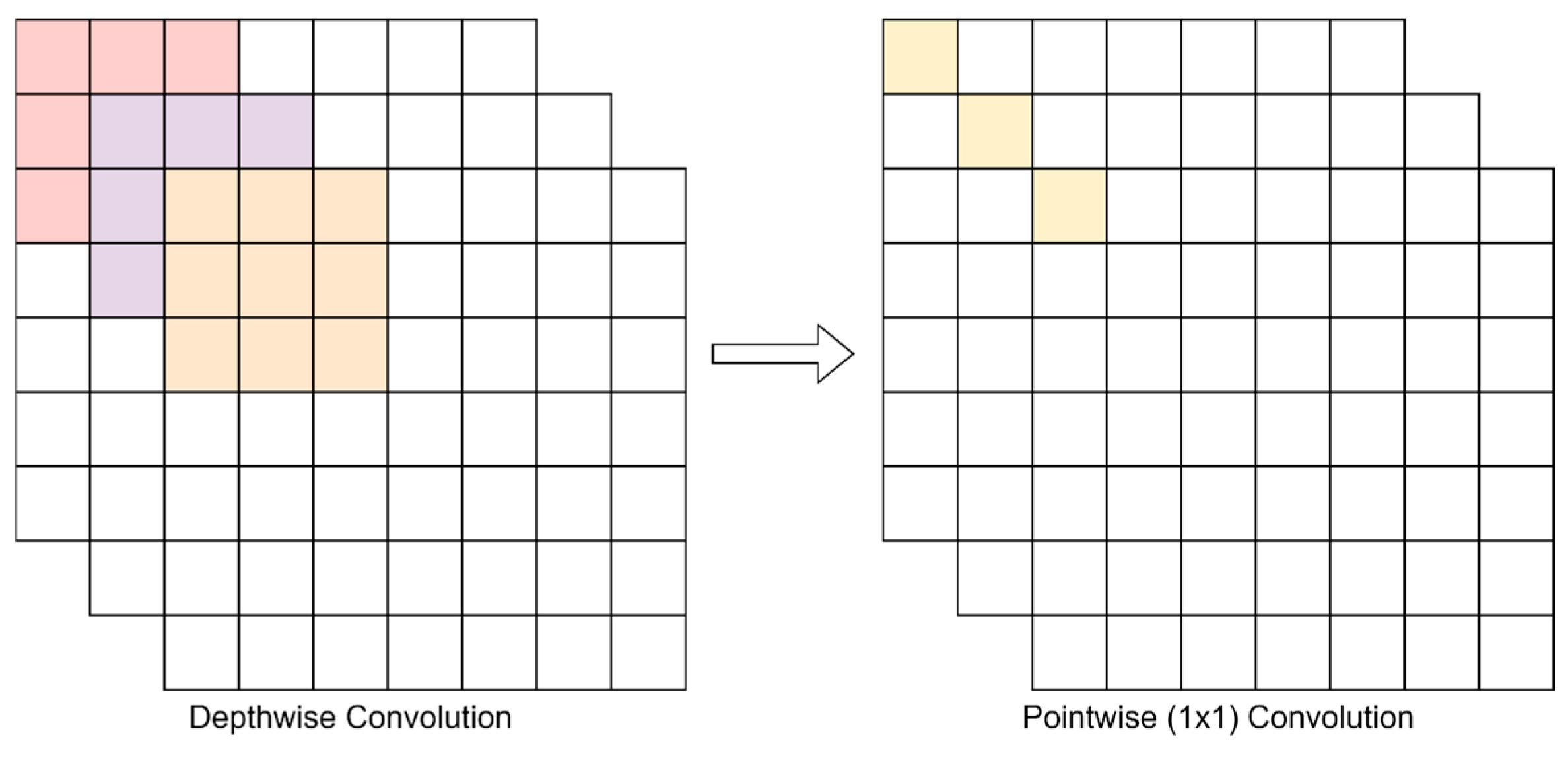
4.1.1. Depthwise Separable Convolution

We built a new residual block to lower the parameters and increase the performance of the network using depthwise separable convolution layers inspired by Mobilenet [52] for mobile devices and embedded vision applications. Depthwise separable convolution [53] is illustrated in Figure 11. Depthwise separable convolution performed pointwise (1 × 1) convolution following depthwise convolution, which was performed using an independent kernel for each channel. For example, for an input image of shape (7 × 7 × 3), convolution with 3 kernels with shape (3 × 1 × 1) is performed. Each kernel iterates on only one channel of the image, which produces an output of shape (5 × 5 × 1), and then all the outputs are stacked to create an output of shape (5 × 5 × 3). This process is called depthwise convolution. Then pointwise convolution is performed to increase the depth of the output by convoluting with a kernel with shape (1 × 1 × depth). If the depth is 32, after the pointwise convolution, the output shape would be (5 × 5 × 32), which is equivalent to convolution with 32 filters of shape (5 × 5). This results in slightly less performance than the traditional convolution, but the number of parameters is greatly reduced, which is essential in multi-stage and real-time applications, as in our case.

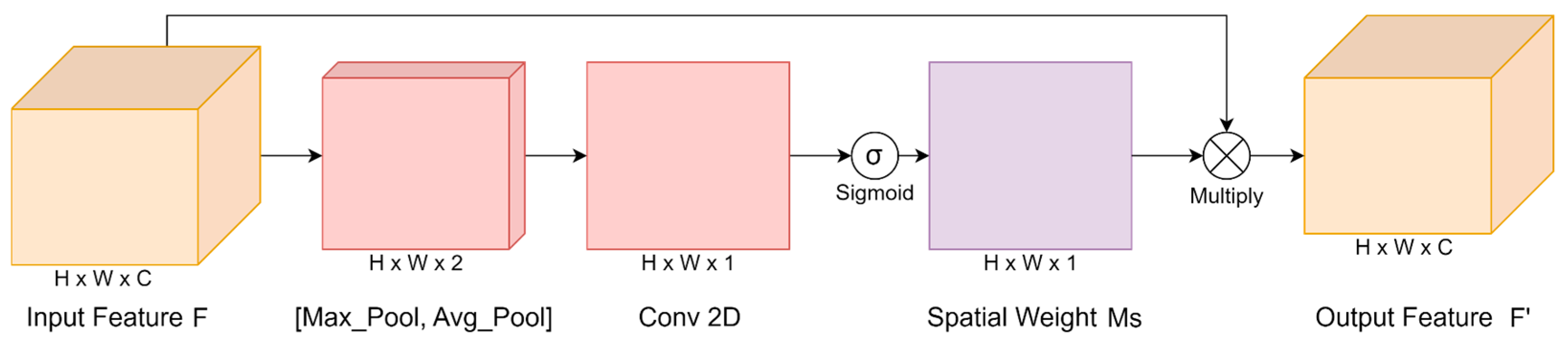
4.1.2. Spatial and Channel Attention Modules

Spatial and channel attention modules are added at each hourglass stage to enhance the feature maps extracted from the network. Since our main focus is to obtain accurate output predictions for the text classes, we add the attention modules to the hourglass network so that they contribute to the best AP (average precision) for the text object classes. We found that the best position to place the attention modules is at the end of the encoder stage before the bottleneck layer for the channel attention, and at the end of the decoder stage at the final feature maps before the output prediction heads for the spatial attention.

The intermediate feature map$F$ of dimension $C\times H\times W$ is passed through a 2D spatial attention weights $Ms$ and channel attention weights $Mc$ of dimension $1\times H\times W$ and $C\times 1\times 1$, respectively. Here, the attention maps/weights are element-wise multiplied with the original feature map F to obtain the refined feature map $F^{\prime }$ and $F^{″}$ as shown in Equation (3).

$$\begin{gathered} {\mathrm{F}}^{\prime }={\mathrm{M}}_s\left(\mathrm{F}\right)\otimes \mathrm{F} \\ {\mathrm{F}}^{″}={\mathrm{M}}_c\left(\mathrm{F}\right)\otimes \mathrm{F} \end{gathered}$$

(3)

The process of obtaining spatially refined features using the spatial attention module is illustrated above in Figure 12. ${\mathrm{F}}_{\mathrm{a}\mathrm{v}\mathrm{g}}^{\mathrm{s}}$ and ${\mathrm{F}}_{\mathrm{m}\mathrm{a}\mathrm{x}}^{\mathrm{s}}$, the global average pooling and global max pooling operations across the channel axis, are used to reduce the feature dimensions from $C\times H\times W$ to $1\times H\times W$ for spatial attention. Avg-Pooling is a mechanism that optimizes a feature map’s spatial size while also providing the network with translation invariance. However, in the attention modules, it is performed over the channel axis by selecting the average pixel value out of all the channels from the feature to reduce the dimension of the feature to a single dimension. Similarly, Max-Pooling is performed over the channel axis by selecting the maximum pixel value out of all the channels. Equation (4) illustrates how these 2D vectors are concatenated, sent to a (3 × 3) convolution filter, and then used in sigmoid activation to learn the inter-spatial relationship and create the spatial attention map $Ms$ of dimension, $1\times H\times W$.

$$\begin{array}{c}{\mathrm{M}}_s\left(\mathrm{F}\right)=\sigma \left(f^{3\times 3}\left(\left[\mathrm{A}\mathrm{v}\mathrm{g}\mathrm{P}\mathrm{o}\mathrm{o}\mathrm{l}\left(\mathrm{F}\right);\mathrm{M}\mathrm{a}\mathrm{x}\mathrm{P}\mathrm{o}\mathrm{o}\mathrm{l}\left(\mathrm{F}\right)\right]\right)\right)\\ =\sigma \left(f^{3\times 3}\left(\left[{\mathrm{F}}_{\mathrm{a}\mathrm{v}\mathrm{g}}^{\mathrm{s}};{\mathrm{F}}_{\mathrm{m}\mathrm{a}\mathrm{x}}^{\mathrm{s}}\right]\right)\right)\end{array}$$

(4)

where σ denotes the sigmoid function, $f^{3\times 3}$is the convolution filter size, $\mathrm{A}\mathrm{v}\mathrm{g}\mathrm{P}\mathrm{o}\mathrm{o}\mathrm{l}\left(\mathrm{F}\right)$ is the average pooling function, and $\mathrm{M}\mathrm{a}\mathrm{x}\mathrm{P}\mathrm{o}\mathrm{o}\mathrm{l}\left(\mathrm{F}\right)$ is the maximum pooling function. We use the number of filters as 16, 32, and 64 during convolution. Following sigmoid activation, these attention maps, which are effectively weighted spatial maps with values ranging from 0 to 1, are multiplied by the original feature map according to Equation (3) to produce the refined spatial attentive feature map.

Figure 13 above shows how to use the channel attention module to obtain channel-wise refined features. Rather than using the traditional way to select the kernel for channel weight determination in the channel attention module, we employ the Efficient Channel Attention Network (ECANET) [47]. The authors claim that it is an enhancement over Squeeze-and-Excitation Attention (SENET) [54], where dimensionality reduction and dependent cross-channel interaction are resolved. The channel weights are learned by the SENET in relation to other channels, not in an independent manner. This is resolved by the ECANET by cross-channel interaction with regard to all other channels in this neighborhood and adaptive local neighborhood size 8. Similar to the SENET, the feature maps are initially refined by using global max pooling to lower the feature map’s dimension from $C\times H\times W$ to $C\times 1\times 1$. After that, it is passed through an adaptive kernel, the size of which describes the neighborhood size, as it slides across this space. It is a one-dimensional convolutional, with a kernel size $k$ that is defined by the following formula and adaptive to the global channel space $C$:

$$k=\psi \left(C\right)={\left|{\displaystyle \frac{{\log }_2\left(C\right)}{\gamma }}+{\displaystyle \frac{b}{\gamma }}\right|}_{odd}$$

(5)

$$\begin{array}{c}{\mathrm{M}}_c\left(\mathrm{F}\right)=\sigma \left(f^{3\times 3}\left(\left[\mathrm{A}\mathrm{v}\mathrm{g}\mathrm{P}\mathrm{o}\mathrm{o}\mathrm{l}\left(\mathrm{F}\right);\mathrm{M}\mathrm{a}\mathrm{x}\mathrm{P}\mathrm{o}\mathrm{o}\mathrm{l}\left(\mathrm{F}\right)\right]\right)\right)\\ =\sigma \left(f^{3\times 3}\left(\left[{\mathrm{F}}_{\mathrm{a}\mathrm{v}\mathrm{g}}^{\mathrm{s}};{\mathrm{F}}_{\mathrm{m}\mathrm{a}\mathrm{x}}^{\mathrm{s}}\right]\right)\right)\end{array}$$

(6)

where $\mathrm{A}\mathrm{v}\mathrm{g}\mathrm{P}\mathrm{o}\mathrm{o}\mathrm{l}\left(\mathrm{F}\right)$ is the average pooling function and $\mathrm{M}\mathrm{a}\mathrm{x}\mathrm{P}\mathrm{o}\mathrm{o}\mathrm{l}\left(\mathrm{F}\right)$ is the maximum pooling function, and ${\left|t\right|}_{odd}$ denotes the nearest odd number of t. We have set γ to 2 and b to 1, in that order. In other words, when mapping the per-channel attention weights, k basically gives the size of the local neighborhood area that will be utilized to record cross-channel interaction. In essence, the function ψ(C) uses the closest odd number as the 1D convolutional kernel size. Because of this, high-dimensional channels interact over a greater range with this mapping ψ, while low-dimensional channels interact over a shorter range with a nonlinear mapping. The subsequent phase bears similarities to spatial attention in that it involves subjecting the features to sigmoid activation. This yields the final channel attention map, which is subsequently multiplied by the initial feature map to obtain the updated feature map. The model can learn “what” and “where” to look in the image by applying the attention modules, which will result in the best performance.

4.2. Text Character Recognition

For OCR, we use the image-based sequence model, which converts image features into sequential features using the RNN and CTC layers proposed in [55]. Figure 14 illustrates the post-processing steps, which involve localizing the words from the text class heatmaps. The bounding boxes for all the objects in the scene are calculated from the heatmap, size, and offset predictions. For OCR, only the text classes are considered, and a mask is created for the character-level bounding box predictions. There are a total of eight text classes, such as place names, motorway names, information in Japanese and English, distance numbers, and motorway numbers. Then the multiplication operation is performed between the text mask and the input image to obtain the image containing only the text. It is followed by binary and Otsu thresholding operations using OpenCV functions. Then morphology and dilation operations are performed to clean and connect the components based on the kernel size. It can be seen that even when some of the character detection fails, an appropriate dilation kernel size is chosen based on the type of text class, and then it is grouped into words. We follow a fixed dilation kernel size for each text class based on the average length of words used during the text augmenting step. There is scope to improve on this technique of grouping words dynamically. It is followed by a contour detection operation to produce the word-level bounding boxes, which are then used to crop the words from the image. These operations are performed for each text class separately. The image shown below represents combining all the masks into a single image for illustration purposes. Some of the challenges faced in the post-processing steps are discussed in Section 5.2.2.

4.2.1. Generate OCR Data

We generate random images and labels for training the OCR model. For the images, we generate random texts with matching font styles similar to the ones used to generate 3D sign boards for English characters, numbers, and Japanese characters. The images are generated by writing the texts of various lengths on the empty NumPy arrays with 10 degrees of rotation using OpenCV functions along with their corresponding labels, where each character is mapped from text to integers and padded with −1 to fill the maximum string length for training. The image dimension is since a grayscale image is used. Some examples of generated images for OCR model training are illustrated in Figure 15. The maximum length of the text is set to 8 with a timestep of 32 for performance reasons. The character list length used to generate images is 1647, consisting of the alphabets a-z, A-Z, numbers 0–9, and 1585 Japanese kanji based on the frequent occurrences while creating text augmentation for the 3D dataset.

4.2.2. Optical Character Recognition Model

Figure 16 illustrates the overview of the OCR model developed to recognize the detected texts. Convolutional networks are used to extract features from the image first, then reshape and density are used to reduce the feature vector dimensions. Then, the bidirectional LSTM is used to process sequential data. Convolutional filters, max-pooling, and fully connected layers from a conventional CNN model with a Resnet backbone are used to build the convolutional feature extraction component. Dropouts are only utilized in full-connected layers, and max-pooling units are used after each convoluted and full-connected layer. These components are used to move a sub-window across the text image in order to extract a feature sequence from an input image. The final feature size is (64 × 512), which is condensed into (64 × 32), where each feature is a time step of input for the recurrent layers and consists of 512 vector elements. The horizontally divided image features are the sequential data fed into the LSTM.

The recurrent connection uses historical contextual information by allowing information from previous inputs to stay in the internal states of the network. LSTM is a type of RNN that solves the vanishing gradient problem and is able to recognize long-term dependencies. The memory blocks that make up the LSTM layer are a collection of blocks that are connected recurrently. Three multiplicative gate units regulate the activation of a set of internal units called cells that make up each block. The gates allow for long-term information storage and access within the cells. Future and past contextual information is useful for many tasks, including text and voice recognition. However, traditional LSTM can only leverage previous contextual data in one way. Bi-directional LSTM (BLSTM) [56], which can learn long-range context dynamics in both input directions, can be used to get around this. The resultant product the output of a given image is transformed by the dense layer into an array representing the number of horizontal steps and character labels in the shape of 32 × 1648. Here, 32 represents the time steps for the CTC layer, and 1648 represents the maximum number of labels.

4.2.3. CTC Loss

CTC loss [57] is used to match the input segments into the desired sequence. CTC aligns a probability output sequence with the label sequence. In text recognition systems, the transcription layer is constructed on top of the recurrent layers to carry out segmentation. The character set is represented by the notation $C^{\prime }=C\cup \left\{blank\right\}$, where $C$ is a fixed set of labels and “$blank”$ stands for no labels. Multiplying the probabilities of labels along this path yields the conditional probability of a path $\pi$ across the lattice of output labels over all time steps for an input sequence of length T, $x=x_1,x_2,\dots ,x_T$

$$p\left(\pi ∣x\right)=\prod _{t=1}^{T}p\left({\pi }_t,t∣x\right)$$

(7)

where the path $\pi$ label at time t is represented by ${\pi }_t$t. A reduction procedure, represented by the letter B, extracts the label sequence from a path by first eliminating duplicate labels and then eliminating any blanks in the path (e.g., B(_hh_e_ll_lll_oo_) = B(_h_ee_l_ll_o) = hello). The overall probability of all the paths, where each path is converted into this label sequence by B, is the likelihood of a label sequence l from an input sequence x. It appears as follows:

$$p\left(\begin{array}{c}l\mid x\end{array}\right)=\sum _{\pi :B\left(\pi \right)=l} p\left(\begin{array}{c}\pi \mid x\end{array}\right)$$

(8)

The best label is decoded by

$$l_{max}=B\left({\pi }_{max}\right);{\pi }_{max}^t=\arg \underset{k}{max} \left(y_k^t\right),t=1\dots T$$

(9)

5. Experiments and Results

5.1. Training

For the first stage, we train on an input resolution of 512 × 512, which yields an output resolution of 128 × 128 for the modified hourglass network of stride 4. Data augmentation was not used since the rotations and scaling were performed while generating the synthetic dataset. The Adam [58] optimizer was used to optimize the overall loss function. A batch size of 32 with an NVIDIA GeForce RTX 3090 GPU and a learning rate of 2.5 × 10⁻⁴ is used for 150 epochs and decreased in steps of 0.1 if there is no improvement in the validation set for 5 epochs.

For the second stage, we train on an input resolution of 128 × 32, which yields an output resolution of 32 × 1648 for the Conv + LSTM network. Data augmentation of scaling and rotation of 10 degrees in both directions was performed. The Adam optimizer was used to optimize the CTC loss. A batch size of 256 with an NVIDIA GeForce RTX 3090 GPU (NVIDIA, Santa Clara, CA, USA) and a learning rate of 1 × 10⁻⁴ is used for 50 epochs and decreased in steps of 0.1 if there is no improvement in the validation set for 10 epochs.

The depth map prediction head is predicted using Mean Absolute Error (MAE) or L1 distance regression loss, while the Gaussian heatmap, width-height, and offset prediction heads are predicted using Mean Squared Error (MSE) or L2 distance regression loss, according to the equation. To update the model weights according to Equations (10) and (11), where $y_i$ is the ground truth, ${\widehat{y}}_i$ is the prediction, and is the total number of samples for a given batch, one can find the mean square error (MSE) by calculating the squared pixel-wise difference between the predicted heatmap and the ground-truth heatmap, and the mean absolute pixel-wise difference between the predicted output and the ground-truth.

$$MSE={\displaystyle \frac{1}{N}}\sum _{i=1}^N (y_i-{\widehat{y}}_i{)}^2$$

(10)

$$MAE={\displaystyle \frac{1}{N}}\sum _{i=1}^N |y_i-{\widehat{y}}_i|$$

(11)

The total loss $L_T$of the object detection model is shown in Equation (12). Here, $L_{hm}$ represents the heatmap loss, $L_{wh}$ and ${\lambda }_{wh}$ represents the width-height loss and weights, $L_{off}$ and ${\lambda }_{off}$ represents the x-y offset loss and weights, $L_{dm}$ and ${\lambda }_{dm}$ represents the depth-map loss and weights.

$$L_T=L_{hm}+L_{wh}{\lambda }_{wh}+L_{off}{\lambda }_{off}+L_{dm}{\lambda }_{dm}$$

(12)

The loss weight values for ${\lambda }_{wh}$, ${\lambda }_{off}$, ${\lambda }_{dm}$ are 5, 5, and 0.5, respectively. These values are decided based on the maximum model performance for the text class heatmap regression.

5.2. Qualitative Analysis

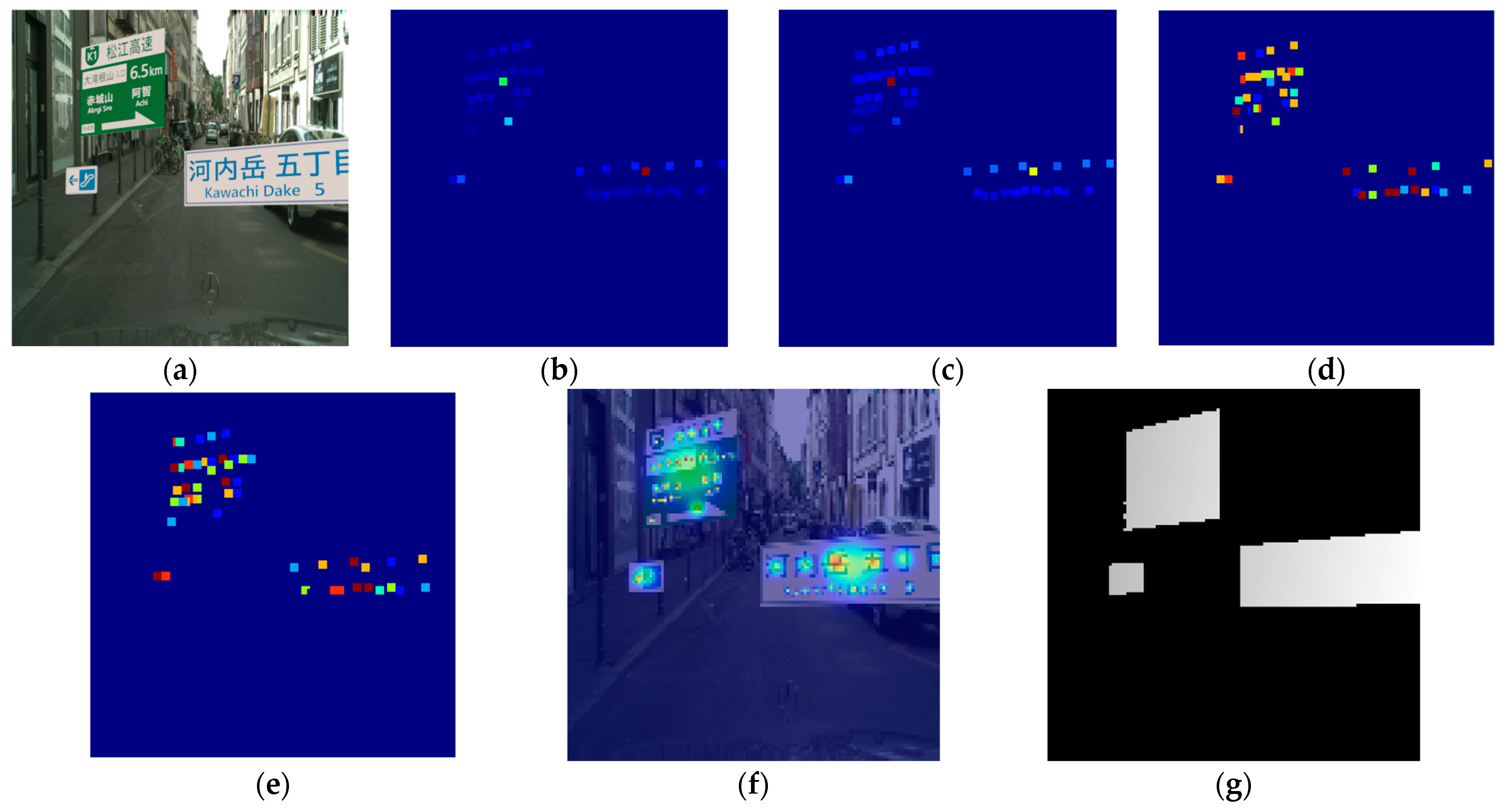
5.2.1. Heatmap Regression and Bounding Box Predictions

Figure 17 illustrates the predictions of the modified two-stage hourglass model. The object center points are decoded from each class of confidence maps by performing the argmax and using a threshold value rather than non-maximum suppression for faster inference. Now that the center coordinate values are available for the downsampled output, the upsampled center coordinates are found by subtracting the offset error given by the offset prediction array. Similarly, the width and height of the objects are decoded from the width-height prediction array. From the depth map, the approximate distance of the sign boards is calculated.

Figure 18 illustrates some of the bounding box predictions of easy samples decoded from the prediction heads of the modified two-stage hourglass model. Figure 18a–d shows various attribute class bounding boxes located within the general information sign board class. Figure 18e–h shows the attribute class bounding boxes for national highway, prefectural, regulatory, and warning sign board classes.

Figure 19 illustrates some of the challenges faced during the bounding box predictions of hard samples. Figure 19b–d,g show some cases where English alphabets and numbers are missed because of very small object sizes and tilted sign boards. Figure 19a,e–h show some cases where the text or arrow attribute appears in the exact center of the outer object category. The object prediction heads can only hold one value per pixel, and as a result, the model learns either the text size or the larger object size. This issue can be resolved using extra prediction head channels for holding the main object (outer) and the attributes (inner), which increase the model parameters, or by using sliding-window techniques. The issue of objects within objects is not addressed in this paper because of the performance issues caused by the need for extra prediction heads. However, in the case of text attributes that were missed in between the words, the problem is resolved during the post-processing stage when converting the characters into words using morphology, dilation, and contour detection. We set the dilation filter size to match the word length required for detection.

Figure 20 illustrates the depth map predictions for some of the test images. We set the maximum distances up to 100 m while creating the dataset, and hence the model can learn to estimate depths up to 100 m. Nearer objects have brighter pixels, and farther objects have darker pixels. The depthmap pixel values are denormalized to find the estimated distance of the object.

Figure 21 illustrates the bounding box predictions for some of the real images and video frames from the in-vehicle camera. There are some missed predictions for smaller text characters. Figure 21a–d shows the predictions for real images; Figure 21e–h shows the predictions for video frames; and Figure 21i–l shows the missed predictions of texts when the signboard is farther, smaller, or of poor quality. The outermost bounding box class predictions seem to be stable for almost all the cases in the real-world dataset. There is definitely room for improvement in the model to detect objects that are smaller.

Figure 22 illustrates the encoder stage’s convolution filter outputs with and without attention blocks for the modified hourglass model. It is visible how the current spatial and channel attention mechanisms help the model learn better features. The attention layers give better filter responses, focusing more on the object of interest.

5.2.2. Text Recognition

Since we have character-level annotations, the goal is to group them into words before they are fed into the OCR model for recognition. Figure 23 illustrates the post-processing outputs of easy samples after the text heatmap regression discussed in Section 5.2.1. Figure 23a–d shows the easy predictions with clean horizontal texts without tilted signboards. Figure 24 shows the challenging scenarios when the horizontal texts are rotated or tilted. Figure 24a–d shows the dilation masks for all the text classes combined for hard samples. Figure 24e–h shows the corresponding word grouping performed in the post-processing step. These images, when cropped for the OCR model, lead to poor character recognition. OCR for rotated images is still a challenging task in the field of AI. We fixed this issue to some extent, as shown in Figure 24i–l, using improved contour masking, but with the penalty of increased post-processing time. Figure 25 illustrates the prediction differences between the YOLOv3 and our model. It can be seen that the YOLOv3 model performs well on large and medium objects, whereas our anchorless model performs well on small objects. It is safe to say that our model performs well on small objects, in our case, text characters.

Table 1. OCR model predictions for easy and hard samples.

Easy Samples	CTC Output	Decoded Label	Hard Samples	CTC Output	Decoded Label
	[30, 49, 34, 45]	EXIT		[35, 28, 45, 20]	XeV
	[53, 53, 36, 12]	11 Km		[28, 42]	CQ
	[40, 10, 4, 19, 14]	Oketo		[]
	[55, 54, 10, 12]	32 km		[50, 1176]	Y口
	[126, 407]	五木		[55, 19, 40, 13, 20]	3tOnu
	[362, 564, 407, 1304]	香ノ木山		[28, 60, 48, 10]	C8Wk

illustrates some of the OCR model predictions for easy and hard samples. “CTC Output” indicates the labels predicted by the OCR model, which are then decoded into words from the dictionary indicated by “Decoded Label”. The model fails to detect texts that are very small because of poor image quality after cropping. The OCR dataset was generated randomly up to a maximum length of eight. Better predictions may be obtained if the dataset is generated with similar words used when text augmenting the 3D model dataset. We found that the model is more accurate for English alphabets compared to Japanese kanji characters.

5.3. Quantitative Analysis

Precision and recall metrics are used to measure the effectiveness of the first-stage model bounding box predictions, which are given by Equations (13) and (14).

$$Precision={\displaystyle \frac{TP}{TP+FP}}$$

(13)

$$Recall={\displaystyle \frac{TP}{TP+FN}}$$

(14)

To evaluate the weight-reduced and attention networks,

Table 2. Validation set mAP for the various models. (# Params is the total number of parameters).

Network Architecture	# Params	mAP@0.5 (Mean)
Hourglass (Baseline)	192.63 M	0.783
YOLOv3	62.49 M	0.723
YOLOv9e	58.1 M	0.833
Hourglass + Depthwise Separable	28.20 M	0.778
Hourglass + Depthwise Separable + Attention	28.25 M	0.819

shows the experimental result obtained by constructing a double-stack hourglass network, where the number of parameters in the table represents the total number of parameters. The mean average precision is calculated as the mean over all the 183 classes of objects. The number of parameters is greatly reduced using the depthwise separable convolution. Also, the inference time is improved by converting the model into TensorFlow Lite for mobile and embedded devices. The model weights are converted into 16-bit floating point and 8-bit unsigned integer values using the quantization technique. This will reduce the model size by 2 and 4, with the least impact on model accuracy and latency. The modified model has a mAP of 81.9%, which is a 4.4% improvement over the baseline centernet model and a 6.37% improvement over the YOLOv3 [59] model. The YOLOv9e [60] provides a mAP of 83.3%, surpassing all the models. Default training parameters are used as per the original papers for Yolo training without changing any hyperparameters. The YOLO models were used to compare our model with the state-of-the-art models, and the tuning of hyperparameters is out of the scope of this paper. The inference time is calculated for the heatmap prediction stage and the post-processing stage after GPU warmup. The post-processing stage time depends on the number of text characters present in the input image. The mean time of a single batch is noted in the below table.

Table 3. Validation set AP for top object classes.

Object Class	AP@0.5	AP@0.75
Japanese Place Names	0.851	0.695
English Place Names	0.822	0.670
Distance Numbers	0.813	0.645
Expressway Numbers	0.808	0.621
General Information	0.78	0.617

shows the average precision values for the top five object classes, which are the text classes since the number of objects in these classes is comparatively higher.

Table 4. Validation set inference times for the various models. Our model provides better inference speed compared to the YOLOv3 model.

Network Architecture	Inference Time
Hourglass (Baseline)	0.174 s
YOLOv3	0.230 s
YOLOv9e	0.039 s
Hourglass + Depthwise Separable	0.139 s
Hourglass + Depthwise Separable + Attention	0.157 s
Hourglass + Depthwise Separable + Attention + Find Peaks	0.225 s
Hourglass + Depthwise Separable + Attention + Find Peaks + Post-Process	0.267 s

shows the average inference times for a batch of validation datasets. The inference times of the models are 0.174 s for the baseline model, 0.23 s for the YOLOv3 model, 0.157 s for our model, and 0.039 s for the YOLOv9 model. There is room for improvements in the model speed for our anchorless model in the future. Nevertheless, the YOLOv9 model has better accuracy and faster inference time compared to any of the models under study but comes with the cost of a higher number of parameters.

Figure 26 illustrates the total loss curves for the object detection model. The validation loss improved until epoch 350, then the training was stopped at 500 epochs to avoid overfitting, and the best weights for the validation loss were saved.

Table 5. Results for validation sets in a modified double-stack hourglass network. (# Params is the total number of parameters).

Network Architecture	# Params	Accuracy	Inference Time	Inference Time + CTC Decode
OCR 1	5.95 M	92.4%	0.027 s	0.031 s

shows the average inference times for a batch of validation datasets. The inference time of the model is 0.031 s for the OCR model.

Figure 27 illustrates the loss curves for the text recognition model. The validation loss improved until epoch 50, then the training was stopped at 60 epochs to avoid overfitting, and the best weights for the validation loss were saved. Around 500 k samples were used to train the OCR model, hence the faster convergence. However, the images while predicting are different from the training dataset but have similar fonts.

6. Conclusions

In this paper, we developed a two-stage anchorless object detection model with text recognition for 3D synthetic traffic sign boards. Our model is further tuned by refining the feature maps using spatial and channel attention modules to yield better predictions, especially for the text classes. Also, we use lightweight convolution filters to reduce the model parameters and improve the performance in real-time applications. Furthermore, our dataset generated from the 3D models is more realistic, mimicking real-world lighting, environment, and weather conditions. The OCR model is capable of recognizing numbers and Japanese and English texts of variable lengths. Our approach to traffic signboard detection using 3D models with the capabilities of extracting various object attributes such as texts, numbers, and direction marks along with depth maps makes it suitable for practical scenarios where more meaningful information can be derived from a 2D image. In summary, this paper’s contributions extend beyond the development of a custom object detection model, offering insights and methodologies that may be applicable to other domains that require the processing of large 3D datasets. We aim to contribute to machine vision by facilitating the development of more meaningful and efficient solutions for real-world applications.

References

1. Denninger, M.; Winkelbauer, D.; Sundermeyer, M.; Boerdijk, W.; Knauer, M.W.; Strobl, K.H.; Humt, M.; Triebel, R. BlenderProc2: A Procedural Pipeline for Photorealistic Rendering. J. Open Source Softw. 2023, 8, 4901. [Google Scholar] [CrossRef]
2. Community, B.O. Blender—A 3D Modelling and Rendering Package. Stichting Blender Foundation, Amsterdam: Blender Foundation. 2018. Available online: https://www.blender.org (accessed on 15 April 2022).
3. Haas, J.K. A History of the Unity Game Engine. Ph.D. Thesis, Worcester Polytechnic Institute, Worcester, MA, USA, 2014. Available online: https://www.unity.com (accessed on 15 April 2022).
4. Richter, S.R.; Vineet, V.; Roth, S.; Koltun, V. Playing for Data: Ground Truth from Computer Games. In Computer Vision—ECCV 2016, Proceedings of the 14th European Conference, Amsterdam, The Netherlands, 11–14 October 2016; Leibe, B., Matas, J., Sebe, N., Welling, M., Eds.; Lecture Notes in Computer Science; Springer International Publishing: Cham, Switzerland, 2016; pp. 102–118. [Google Scholar]
5. Tremblay, J.; Prakash, A.; Acuna, D.; Brophy, M.; Jampani, V.; Anil, C.; To, T.; Cameracci, E.; Boochoon, S.; Birchfield, S. Training Deep Networks with Synthetic Data: Bridging the Reality Gap by Domain Randomization. In Proceedings of the IEEE/CVF Conference on Computer Vision and Pattern Recognition Workshops (CVPRW), Salt Lake City, UT, USA, 18–22 June 2018; pp. 1082–10828. [Google Scholar]
6. Baek, Y.; Lee, B.; Han, D.; Yun, S.; Lee, H. Character Region Awareness for Text Detection. In Proceedings of the IEEE/CVF Conference on Computer Vision and Pattern Recognition (CVPR), Long Beach, CA, USA, 15–20 June 2019; pp. 9357–9366. [Google Scholar]
7. Lin, T.Y.; Maire, M.; Belongie, S.; Hays, J.; Perona, P.; Ramanan, D.; Dollár, P.; Zitnick, C.L. Microsoft COCO: Common Objects in Context. In Proceedings of the 13th European Conference on Computer Vision (ECCV), Zurich, Switzerland, 6–12 September 2014; pp. 740–755. [Google Scholar]
8. Ren, S.; He, K.; Girshick, R.B.; Sun, J. Faster R-CNN: Towards Real-Time Object Detection with Region Proposal Networks. IEEE Trans. Pattern Anal. Mach. Intell. 2015, 39, 1137–1149. [Google Scholar] [CrossRef] [PubMed]
9. Redmon, J.; Divvala, S.; Girshick, R.; Farhadi, A. You only look once: Unified, real-time object detection. In Proceedings of the IEEE Conference on Computer Vision and Pattern Recognition, Las Vegas, NV, USA, 27–30 June 2016; pp. 779–788. [Google Scholar]
10. Law, H.; Deng, J. CornerNet: Detecting Objects as Paired Keypoints. Int. J. Comput. Vis. 2018, 128, 642–656. [Google Scholar] [CrossRef]
11. Duan, K.; Bai, S.; Xie, L.; Qi, H.; Huang, Q.; Tian, Q. CenterNet: Keypoint Triplets for Object Detection. In Proceedings of the 2019 IEEE/CVF International Conference on Computer Vision (ICCV), Seoul, Republic of Korea, 27 October–2 November 2019; pp. 6568–6577. [Google Scholar]
12. Zhou, X.; Zhuo, J.; Krahenbuhl, P. Bottom-up object detection by grouping extreme and center points. In Proceedings of the IEEE/CVF Conference on Computer Vision and Pattern Recognition, Long Beach, CA, USA, 15–20 June 2019; pp. 850–859. [Google Scholar]
13. Zhou, X.; Wang, D.; Krähenbühl, P. Objects as points. arXiv 2019, arXiv:1904.07850. [Google Scholar]
14. Liu, C.; Li, S.; Chang, F.; Wang, Y. Machine Vision Based Traffic Sign Detection Methods: Review, Analyses and Perspectives. IEEE Access 2019, 7, 86578–86596. [Google Scholar] [CrossRef]
15. Zakir, U.; Leonce, A.N.J.; Edirisinghe, E. Road Sign Segmentation Based on Colour Spaces: A Comparative Study. In Proceedings of the 11th Iasted International Conference on Computer Graphics and Imgaing, Innsbruck, Austria, 17–19 February 2010; pp. 17–19. [Google Scholar]
16. Youssef, A.; Albani, D.; Nardi, D.; Bloisi, D.D. Fast Traffic Sign Recognition Using Color Segmentation and Deep Convolutional Networks. In Advanced Concepts for Intelligent Vision Systems; Blanc-Talon, J., Distante, C., Philips, W., Popescu, D., Scheunders, P., Eds.; Lecture Notes in Computer Science; Springer International Publishing: Cham, Switzerland, 2016; Volume 10016, pp. 205–216. [Google Scholar]
17. Prisacariu, V.A.; Timofte, R.; Zimmermann, K.; Reid, I.; Van Gool, L. Integrating Object Detection with 3D Tracking towards a Better Driver Assistance System. In Proceedings of the 2010 20th International Conference on Pattern Recognition, Istanbul, Turkey, 23–26 August 2010; pp. 3344–3347. [Google Scholar]
18. Saadna, Y.; Behloul, A. An Overview of Traffic Sign Detection and Classification Methods. Int. J. Multimed. Inf. Retr. 2017, 6, 193–210. [Google Scholar] [CrossRef]
19. Rajendran, S.P.; Shine, L.; Pradeep, R.; Vijayaraghavan, S. Real-Time Traffic Sign Recognition Using YOLOv3 Based Detector. In Proceedings of the 2019 10th International Conference on Computing, Communication and Networking Technologies (ICCCNT), Kanpur, India, 6–8 July 2019; pp. 1–7. [Google Scholar]
20. Li, Y.; Li, J.; Meng, P. Attention-YOLOV4: A Real-Time and High-Accurate Traffic Sign Detection Algorithm; Springer: Berlin/Heidelberg, Germany, 2022; pp. 1–16. [Google Scholar]
21. Newell, A.; Yang, K.; Deng, J. Stacked Hourglass Networks for Human Pose Estimation. In Proceedings of the European Conference on Computer Vision, Amsterdam, The Netherlands, 11–14 October 2016; pp. 483–499. [Google Scholar]
22. Soans, R.V.; Fukumizu, Y. Improved Facial Keypoint Regression Using Attention Modules. In Proceedings of the Communi-cations in Computer and Information Science, Frontiers of Computer Vision, Hiroshima, Japan, 21–22 February 2022; pp. 182–196. [Google Scholar]
23. Shivanna, V.M.; Guo, J. Object Detection, Recognition, and Tracking Algorithms for ADASs—A Study on Recent Trends. Sensors 2023, 24, 249. [Google Scholar] [CrossRef]
24. Diwan, T.; Anirudh, G.S.; Tembhurne, J.V. Object detection using YOLO: Challenges, architectural successors, datasets and applications. Multimed. Tools Appl. 2022, 82, 9243–9275. [Google Scholar] [CrossRef] [PubMed]
25. Wang, J.; Chen, Y.; Dong, Z.; Gao, M. Improved YOLOv5 network for real-time multi-scale traffic sign detection. Neural Comput. Appl. 2021, 35, 7853–7865. [Google Scholar] [CrossRef]
26. Chu, J.; Zhang, C.; Yan, M.; Zhang, H.; Ge, T. TRD-YOLO: A Real-Time, High-Performance Small Traffic Sign Detection Algorithm. Sensors 2023, 23, 3871. [Google Scholar] [CrossRef]
27. Liu, H.; Zhou, K.; Zhang, Y.; Zhang, Y. ETSR-YOLO: An improved multi-scale traffic sign detection algorithm based on YOLOv5. PLoS ONE 2023, 18, e0295807. [Google Scholar] [CrossRef] [PubMed]
28. Wang, Y.; Bai, M.; Wang, M.; Zhao, F.; Guo, J. Multiscale Traffic Sign Detection Method in Complex Environment Based on YOLOv4. In Computational Intelligence and Neuroscience; John Wiley & Sons Ltd.: Hoboken, NJ, USA, 2022; p. 5297605. [Google Scholar]
29. Liu, Y.; Shi, G.; Li, Y.; Zhao, Z. M-YOLO: Traffic Sign Detection Algorithm Applicable to Complex Scenarios. Symmetry 2022, 14, 952. [Google Scholar] [CrossRef]
30. Shen, J.; Zhang, Z.; Luo, J.; Zhang, X. YOLOv5-TS: Detecting traffic signs in real-time. Front. Phys. 2023, 11, 1297828. [Google Scholar] [CrossRef]
31. Zhang, K.; Chen, J.; Zhang, R.; Hu, C. A Hybrid Approach for Efficient Traffic Sign Detection Using Yolov8 and SAM. In Proceedings of the 2024 3rd Asia Conference on Algorithms, Computing and Machine Learning, Shanghai, China, 22–24 March 2024; pp. 298–302. [Google Scholar]
32. Luo, Y.; Ci, Y.; Jiang, S.; Wei, X. A novel lightweight real-time traffic sign detection method based on an embedded device and YOLOv8. J. Real Time Image Process. 2024, 21, 24. [Google Scholar] [CrossRef]
33. Liu, X.; Yan, W.Q. Traffic-light sign recognition using capsule network. Multimed. Tools Appl. 2021, 80, 15161–15171. [Google Scholar] [CrossRef]
34. Kumar, A.D. Novel Deep Learning Model for Traffic Sign Detection Using Capsule Networks. arXiv 2018, arXiv:1805.04424. [Google Scholar]
35. Yalamanchili, S.; Kodepogu, K.; Manjeti, V.B.; Mareedu, D.; Madireddy, A.; Mannem, J.; Kancharla, P.K. Optimizing Traffic Sign Detection and Recognition by Using Deep Learning. Int. J. Transp. Dev. Integr. 2024, 8, 131–139. [Google Scholar] [CrossRef]
36. Sheeba, S.; Vamsi, V.M.S.; Sonti, H.; Ramana, P. Intelligent Traffic Sign Detection and Recognition Using Computer Vision. In Intelligent Systems Design and Applications; Abraham, A., Pllana, S., Hanne, T., Siarry, P., Eds.; Springer: Berlin/Heidelberg, Germany, 2024; Volume 1048. [Google Scholar]
37. Chi, X.; Luo, D.; Liang, Q.; Yang, J.; Huang, H. Detection and Identification of Text-based Traffic Signs. Sens. Mater. 2023, 35, 153–165. [Google Scholar] [CrossRef]
38. Kiefer, B.; Ott, D.; Zell, A. Leveraging Synthetic Data in Object Detection on Unmanned Aerial Vehicles. In Proceedings of the 2022 26th International Conference on Pattern Recognition (ICPR), Montreal, QC, Canada, 21–25 August 2022; pp. 3564–3571. [Google Scholar]
39. Premakumara, N.; Jalaeian, B.; Suri, N.; Samani, H.A. Enhancing object detection robustness: A synthetic and natural perturbation approach. arXiv 2023, arXiv:2304.10622. [Google Scholar]
40. Clement, N.L.; Schoen, A.; Boedihardjo, A.P.; Jenkins, A. Synthetic Data and Hierarchical Object Detection in Overhead Imagery. ACM Trans. Multimed. Comput. Commun. Appl. 2021, 20, 1–20. [Google Scholar] [CrossRef]
41. Adobe Inc. Adobe Illustrator. 2019. Available online: https://adobe.com/products/illustrator (accessed on 7 January 2022).
42. Adobe Inc. Adobe Photoshop. 2019. Available online: https://www.adobe.com/products/photoshop.html (accessed on 20 April 2023).
43. The GIMP Development Team. GIMP. 2019. Available online: https://www.gimp.org (accessed on 7 January 2022).
44. Inkscape Project. Inkscape. 2020. Available online: https://inkscape.org (accessed on 7 January 2022).
45. Stallkamp, J.; Schlipsing, M.; Salmen, J.; Igel, C. The German traffic sign recognition benchmark: A multi-class classification competition. In Proceedings of the 2011 International Joint Conference on Neural Networks, San Jose, CA, USA, 31 July–5 August 2011; pp. 1453–1460. [Google Scholar]
46. Yang, Y.; Luo, H.; Xu, H.; Wu, F. Towards real-time traffic sign detection and classification. IEEE Trans. Actions Intell. Transp. Syst. 2016, 17, 2022–2031. [Google Scholar] [CrossRef]
47. Wang, Q.; Wu, B.; Zhu, P.F.; Li, P.; Zuo, W.; Hu, Q. ECA-Net: Efficient Channel Attention for Deep Convolutional Neural Networks. In Proceedings of the 2020 IEEE/CVF Conference on Computer Vision and Pattern Recognition (CVPR), Seattle, WA, USA, 14–19 June 2020; pp. 11531–11539. [Google Scholar]
48. Cordts, M.; Omran, M.; Ramos, S.; Rehfeld, T.; Enzweiler, M.; Benenson, R.; Franke, U.; Roth, S.; Schiele, B. The cityscapes dataset for semantic urban scene understanding. In Proceedings of the IEEE Conference on Computer Vision and Pattern Recognition, Las Vegas, NV, USA, 27–30 June 2016; pp. 3213–3223. [Google Scholar]
49. Cao, Z.; Hidalgo, G.; Simon, T.; Wei, S.; Sheikh, Y. OpenPose: Realtime Multi-Person 2D Pose Estimation Using Part Affinity Fields. IEEE Trans. Pattern Anal. Mach. Intell. 2018, 43, 172–186. [Google Scholar] [CrossRef] [PubMed]
50. Noh, H.; Hong, S.; Han, B. Learning deconvolution network for semantic segmentation. In Proceedings of the IEEE International Conference on Computer Vision, Santiago, Chile, 7–13 December 2015; pp. 1520–1528. [Google Scholar]
51. Badrinarayanan, V.; Kendall, A.; Cipolla, R. SegNet: A Deep Convolutional Encoder-Decoder Architecture for Image Segmentation. IEEE Trans. Pattern Anal. Mach. Intell. 2015, 39, 2481–2495. [Google Scholar] [CrossRef] [PubMed]
52. Howard, A.G.; Zhu, M.; Chen, B.; Kalenichenko, D.; Wang, W.; Weyand, T.; Andreetto, M.; Adam, H. Mobilenets: Efficient convolutional neural networks for mobile vision applications. arXiv 2017, arXiv:1704.04861. [Google Scholar]
53. Chollet, F. Xception: Deep learning with depthwise separable convolutions. In Proceedings of the 2017 IEEE Conference on Computer Vision and Pattern Recognition (CVPR), Honolulu, HI, USA, 21–26 July 2017; pp. 1800–1807. [Google Scholar]
54. Hu, J.; Shen, L.; Albanie, S.; Sun, G.; Wu, E. Squeeze-and-Excitation Networks. In Proceedings of the 2018 IEEE/CVF Conference on Computer Vision and Pattern Recognition, Salt Lake City, UT, USA, 18–22 June 2018; pp. 7132–7141. [Google Scholar]
55. Graves, A.; Fern’andez, S.; Gomez, F.J.; Schmidhuber, J. Connectionist Temporal Classification: Labelling Unsegmented Sequence Data with Recurrent Neural Networks. In Proceedings of the 23rd International Conference on Machine Learning, Pittsburgh, PA, USA, 25–29 June 2006; pp. 369–376. [Google Scholar]
56. Hochreiter, S.; Schmidhuber, J. Long short-term memory. Neural Comput. 1997, 9, 1735–1780. [Google Scholar] [CrossRef] [PubMed]
57. Shi, B.; Bai, X.; Yao, C. An end-to-end trainable neural network for image-based sequence recognition and its application to scene text recognition. IEEE Trans. Pattern Anal. Mach. Intell. 2017, 39, 2298–2304. [Google Scholar] [CrossRef]
58. Kingma, D.P.; Ba, J. Adam: A Method for Stochastic Optimization. arXiv 2014, arXiv:1412.6980. [Google Scholar]
59. Redmon, J.; Farhadi, A. YOLOv3: An Incremental Improvement. arXiv 2018, arXiv:1804.02767. [Google Scholar]
60. Wang, C.; Yeh, I.; Liao, H. YOLOv9: Learning What You Want to Learn Using Programmable Gradient Information. arXiv 2024, arXiv:2402.13616. [Google Scholar]
Figure 1. Various steps involved in the 3D modeling of the dataset.
Applsci 14 06352 g001
Figure 2. Synthetic traffic sign board variations (a) Warning Sign Boards; (b) Urban Expressway Sign Boards; (c) Supplementary Sign Boards.
Applsci 14 06352 g002
Figure 3. Synthetic traffic sign board variations (a) Regulatory Sign Boards; (b) Prefectural Sign Boards; (c) Intersection Sign Boards.
Applsci 14 06352 g003
Figure 4. Synthetic traffic sign board variations (a) National Highway Sign Boards; (b) Expressway Sheild Sign Boards; (c) General Information Sign Boards.
Applsci 14 06352 g004
Figure 5. Synthetic traffic sign board (a) 3D models for GTSDB [47]; (b) 3D models for CTSD [21].
Applsci 14 06352 g005
Figure 6. Simulate adverse weather conditions with Cityscapes [48] dataset as background (a) Rain; (b) Snow; (c) Fog.
Applsci 14 06352 g006
Figure 7. Ground-truth generated for an image (a) Input Image; (b) Height Mask; (c) Width Mask; (d) Offset_x Mask; (e) Offset_y Mask; (f) Gaussian Heatmap (sum on all axis); (g) Depth Map.
Applsci 14 06352 g007
Figure 8. Traffic sign board detection workflow.
Applsci 14 06352 g008
Figure 9. Two-Stage Hourglass model.
Applsci 14 06352 g009
Figure 10. Modified Hourglass module.
Applsci 14 06352 g010
Figure 11. Depthwise separable convolution.
Applsci 14 06352 g011
Figure 12. Spatial attention module.
Applsci 14 06352 g012
Figure 13. Efficient channel attention module [28].
Applsci 14 06352 g013
Figure 14. Post-processing: Character level heatmap to word segments.
Applsci 14 06352 g014
Figure 15. Random grayscale images generated for the OCR model training.
Applsci 14 06352 g015
Figure 16. Optical character recognition model.
Applsci 14 06352 g016
Figure 17. Prediction results of the proposed method for the synthetic dataset. (a) Input image; (b) Width prediction; (c) Height prediction; (d) Offset x prediction; (e) Offset y prediction; (f) Heatmap prediction; (g) Depth map prediction; (h) Bounding Box prediction.
Applsci 14 06352 g017aApplsci 14 06352 g017b
Figure 18. Bounding box predictions for easy samples (ah).
Applsci 14 06352 g018
Figure 19. Bounding box predictions for hard samples (ah).
Applsci 14 06352 g019
Figure 20. Depth map predictions for validation samples (ah).
Applsci 14 06352 g020aApplsci 14 06352 g020b
Figure 21. Bounding box predictions of real images and video frames. (ad) Real images; (eh) Video frames; (il) Hard samples.
Applsci 14 06352 g021
Figure 22. Activation maps of the intermediate layers of hourglass model (a) Without attention modules; (b) With attention modules.
Applsci 14 06352 g022
Figure 23. Character level predictions to word grouping for easy samples (ad).
Applsci 14 06352 g023
Figure 24. Character level predictions to word grouping for hard samples. (ad) Dilation masks; (eh) Character to word grouping; (il) Improved character to word grouping.
Applsci 14 06352 g024
Figure 25. Comparison results of YOLO v3 vs. our model for worst-case conditions. (ad) YOLOv3 predictions; (eh) Our model predictions.
Applsci 14 06352 g025aApplsci 14 06352 g025b
Figure 26. Object detection model training loss curves.
Applsci 14 06352 g026
Figure 27. OCR model training curves (a) Loss curves; (b) Accuracy curves.
Applsci 14 06352 g027