A Study on Three-Dimensional Multi-Cluster Fracturing Simulation under the Influence of Natural Fractures

Abstract

Multi-cluster fracturing has emerged as an effective technique for enhancing the productivity of deep shale reservoirs. The presence of natural bedding planes in these reservoirs plays a significant role in shaping the evolution and development of multi-cluster hydraulic fractures. Therefore, conducting detailed research on the propagation mechanisms of multi-cluster hydraulic fractures in deep shale formations is crucial for optimizing reservoir transformation efficiency and achieving effective development outcomes. This study employs the finite discrete element method (FDEM) to construct a comprehensive three-dimensional simulation model of multi-cluster fracturing, considering the number of natural fractures present and the geo-mechanical characteristics of a target block. The propagation of hydraulic fractures is investigated in response to the number of natural fractures and the design of the multi-cluster fracturing operations. The simulation results show that, consistent with previous research on fracturing in shale oil and gas reservoirs, an increase in the number of fracturing clusters and natural fractures leads to a larger total area covered by artificial fractures and the development of more intricate fracture patterns. Furthermore, the present study highlights that an escalation in the number of fracturing clusters results in a notable reduction in the balanced expansion of the double wings of the main fracture within the reservoir. Instead, the effects of natural fractures, geo-stress, and other factors contribute to enhanced phenomena such as single-wing expansion, bifurcation, and the bending of different main fractures, facilitating the creation of complex artificial fracture networks. It is important to note that the presence of natural fractures can also significantly alter the failure mode of artificial fractures, potentially resulting in the formation of small opening shear fractures that necessitate careful evaluation of the overall renovation impact. Moreover, this study demonstrates that even in comparison to single-cluster fracturing, the presence of 40 natural main fractures in the region can lead to the development of multiple branching main fractures. This finding underscores the importance of considering natural fractures in deep reservoir fracturing operations. In conclusion, the findings of this study offer valuable insights for optimizing deep reservoir fracturing processes in scenarios where natural fractures play a vital role in shaping fracture development.

1. Introduction

Oil and gas resources continue to play a significant role in the global energy landscape. Therefore, there is a pressing need to ramp up the extraction and utilization of these resources [1]. Deep shale oil and gas resources at depths of over 3500 m account for a huge proportion of the current energy structure. Optimizing the construction and exploitation of deep oil and gas resources through construction techniques such as multi-cluster fracturing is a necessary means to achieve efficient exploitation of deep oil and gas resources [2]. It is noteworthy that deep oil and gas reservoirs are often found in high-stress environments with complex fracture characteristics (discontinuous structures such as bedding, joints, and fractures formed by the sedimentation and tectonic processes of deep reservoirs) [3], which significantly affects the effectiveness of reservoir transformation [4,5]. Therefore, an in-depth exploration of the impact of natural fractures on the multi-cluster fracturing construction technology of deep oil and gas reservoirs is of great significance for the development of deep oil and gas resources.

Both theoretical solutions and indoor tests can be used to study the propagation of fracturing fractures. Over the years, various theoretical solution models such as the KGD model, PKN model, and Penny model, among others, have been established through theoretical derivations [2,6,7,8,9,10]. Meanwhile, some scholars have found in their research that there may be multiple control mechanisms in the reservoir due to the influence of fracture toughness and the fracturing injection rate of reservoir rocks. Therefore, a theoretical model for artificial fracture propagation in reservoirs under the influence of comprehensive parameters such as viscosity control and toughness control has been derived. However, the reservoir rock is often assumed to be a homogenous and isotropic medium in theoretical derivation, meaning that the impact of naturally occurring fractures and the growth of numerous fracture groups cannot be considered. Of course, scholars have also conducted extensive physical simulation research using laboratory experimental methods [5,11,12,13,14,15]. In the initial stages, conventional triaxial loading systems were predominantly utilized, focusing on the influence of reservoir geo-stress by controlling surrounding rock and axial pressure. However, real reservoirs typically experience stress conditions under true triaxial stress, prompting some researchers to develop authentic triaxial experimental setups to simulate fracturing from single to multiple clusters. Through these experiments, they have been able to glean insights into the propagation patterns of artificial fractures. Nevertheless, replicating the impact of natural fractures in laboratory settings proves to be a challenge, and further examination is warranted for the transferability of specimen-scale results to reservoir-scale scenarios. Consequently, there is a growing interest in the simulation analysis of reservoir fracturing at the reservoir scale [16,17].

The principle of multi-cluster fracturing in tight reservoirs is illustrated in Figure 1. This method involves creating multiple hydraulic fracture networks in various blocks within the reservoir by strategically establishing multiple perforation positions and adjusting the fluid distribution across different clusters. The overarching objective is to enhance reservoir permeability and facilitate efficient development. Early reservoir fracturing simulations were mainly achieved through finite element methods. Subsequently, considering that reservoir rocks are a discontinuous medium, some new numerical simulation methods were proposed successively, such as the extended finite element method [18], particle flow dispersion element method [19,20], block discrete element method [2], discontinuous element method [21], finite discrete element method (FDEM) [22], etc. These methods make it possible to predict the fracturing construction effect of the target reservoir more accurately, but they have different advantages and limitations. For example, the extended finite element method uses virtual functions to construct a discontinuous displacement field, which can simulate the phenomenon of fracture deflection and propagation inside the element, but it is difficult to simulate the effects of natural fractures and other factors such as fracture bifurcation. The particle flow dispersion element method has an excellent performance in simulating reservoir fracturing at the micro-scale, but it usually assumes that the reservoir is composed of particles, which has great computational limitations and is no longer suitable for reservoir-scale simulation analysis [23,24]. The block discrete element method and finite discrete element method developed in recent years have effectively solved the scale limitations, thus enabling better simulation and evaluation of reservoir fracturing from micro- to macro-scales. Among them, the finite discrete element method [25] assumes that the reservoir is composed of rock blocks and their fractured interfaces (Figure 1). The rock block elements are used to simulate the deformation characteristics of the reservoir matrix during the fracturing process, and the interface elements are used to simulate the propagation of artificial fractures in the reservoir. Meanwhile, with years of development, the characteristics of natural fractures in reservoirs can be described by changing parameters such as the strength and stiffness of different interface elements, thereby achieving fracturing simulation on reservoirs containing natural fractures. Based on the FDEM method, Wu et al. [26] conducted a hydraulic fracturing inversion simulation study considering the natural bedding/fracture interfaces in rocks. Their findings confirmed the viability of utilizing the FDEM to simulate fracture formation in rocks containing such natural features. Additionally, they developed hydraulic fracturing models for reservoir areas considering various heterogeneous structures and conducted a detailed analysis on the impact of factors like natural discrete fractures and large embedded rock blocks on the propagation of hydraulic fractures [27]. Therefore, conducting a simulation study on fracturing in fractured reservoirs using the FDEM proves to be an effective method for unveiling the propagation behavior of hydraulic fractures in reservoir rocks containing natural fractures.

Based on the finite discrete element method (FDEM), this paper establishes a three-dimensional multi-cluster fracturing simulation model considering the number of natural fractures. The conventional quantitative parameters such as fracture area, fracture length, and maximum fracture aperture were used to systematically analyze the expansion law of artificial fractures under the combined influence of natural fractures and multi-cluster fracturing. The numerical model, the comparative analysis results, and the conclusion are presented in Section 2, Section 3, and Section 4, respectively.

2. Numerical Model

This paper uses cohesive elements and rock block elements to construct an FDEM model [28,29,30] and divides cohesive elements into cohesive elements within the matrix and cohesive elements representing natural fractures, thus achieving multi-cluster fracturing modeling of reservoirs containing natural fractures. The detailed modeling equations are as follows.

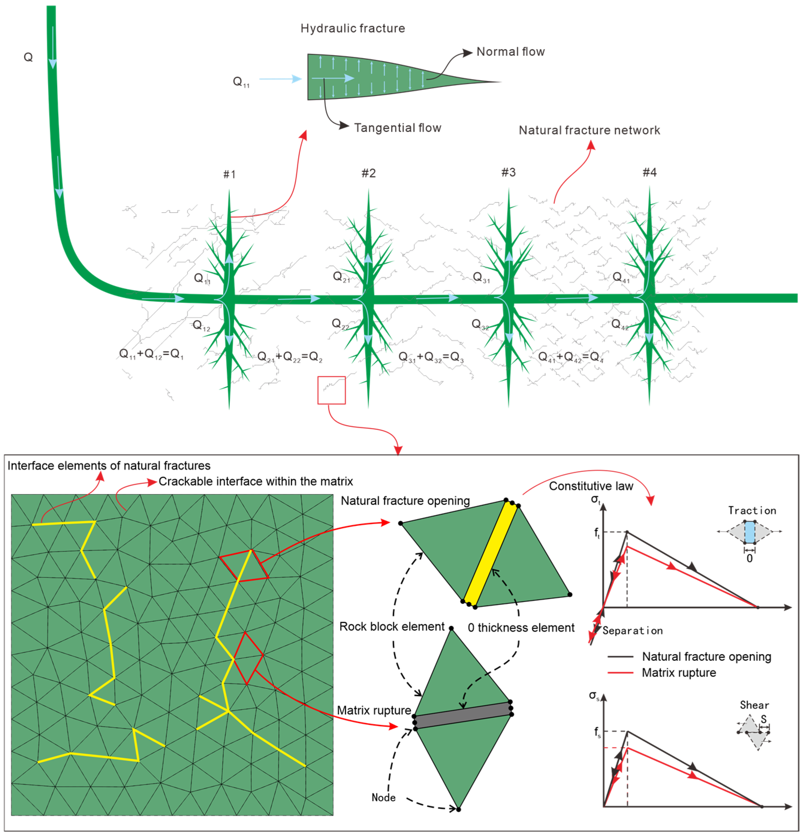
2.1. Simulation Method

Multi-cluster hydraulic fracturing in reservoirs is a typical fluid structure coupling process that involves the interaction between fluids and solids. When considering the interaction between fluids and solids during hydraulic fracturing, the stress balance equation of hydraulic fracturing can be expressed as [31]

$${\displaystyle \underset{V}{\int }\left(\overline{\mathit{\sigma }}-p_w\mathit{I}\right)\delta \mathit{\epsilon }\delta dV=\underset{S}{\int }\mathit{t}·\delta \mathit{v}dS+\underset{V}{\int }\mathit{f}\delta \mathit{v}dV}$$

(1)

where $\overline{\sigma }$ represents the effective stress matrix, MPa; $p_w$ denotes the pore pressure, MPa; $\delta \mathit{\epsilon }/s^{-1}$ is the virtual strain rate matrix; $\mathit{t}$ is the surface force matrix, N/m²; ${\delta }_{\mathit{v}}$ (m/s) and $\mathit{f}$ (N/m³) are the virtual velocity matrix and the physical force matrix.

During the fracturing process, fluid density and matrix porosity influence the behavior of the fluid within the reservoir. The fluid continuity equation captures the conservation of mass during this process, providing a mathematical representation of the fluid’s movement and distribution. It enables a more accurate description of the fluid flow dynamics within the reservoir [32].

$${\displaystyle \frac{d}{dt}}\left(\underset{V}{\int }\left({\displaystyle \frac{{\rho }_w}{{\rho }_w^0}}ndV\right)\right)+\underset{S}{\int }{\displaystyle \frac{{\rho }_w}{{\rho }_w^0}}n\mathit{n}·v_{w}dS=0$$

(2)

where $J$ represents the volume change ratio, dimensionless; ${\rho }_w$ is the fluid density, kg/m³; $n_w$ is the void ratio, dimensionless; and $v_w$ is the fluid seepage velocity, m/s.

It is important to mention that the fracturing process also involves the influence of fluid seepage within the matrix. The seepage behavior of reservoir rocks during fracturing can be calculated using Darcy’s law, which determines the velocity and flow rate of fluids through factors such as fluid viscosity, permeability, and pressure gradient [33]:

$${\mathit{v}}_w=-{\displaystyle \frac{1}{n_w\mathit{g}{\rho }_w}}\mathit{k}·\left({\displaystyle \frac{\partial p_w}{\partial \mathit{x}}}-{\rho }_w\mathit{g}\right)$$

(3)

where $\mathit{k}$ represents a permeability matrix, m/s, and $\mathit{g}$ is the gravity acceleration vector, m/s².

As fluid starts to seep into the reservoir rock mass, the influx of fluid will lead to an elevation in pore pressure, consequently facilitating the propagation of microfractures. It is generally believed that before hydraulic fractures open, the cohesive elements used to simulate hydraulic fractures follow a linear elastic relationship [6],

$${\mathit{\sigma }}_{coh}=\left\{\begin{array}{c}{\sigma }_{coh\_n}\\ {\sigma }_{coh\_s}\\ {\sigma }_{coh\_t}\end{array}\right\}={\mathit{K}}_{coh}{\mathit{\epsilon }}_{coh}=\left[\begin{array}{ccc}{K}_{coh\_nn}& K_{coh\_ns}& K_{coh\_nt}\\ K_{coh\_ns}& K_{coh\_ss}& K_{coh\_st}\\ K_{coh\_nt}& K_{coh\_st}& K_{coh\_tt}\end{array}\right]\left\{\begin{array}{c}{\epsilon }_{coh\_n}\\ {\epsilon }_{coh\_s}\\ {\epsilon }_{coh\_t}\end{array}\right\},$$

(4)

where ${\mathit{\sigma }}_{coh}$ denotes the stress vector; ${\mathit{\sigma }}_{coh\_h,} {\mathit{\sigma }}_{coh\_s,} {\mathit{\sigma }}_{coh\_t}$ are the normal stress, the first tangent stress and the second tangent stress, respectively. Here, ${\mathit{K}}_{coh}$ denotes the stiffness matrix; ${\mathit{\epsilon }}_{coh}$ is the strain matrix, and ${\mathit{\epsilon }}_{coh\_n,} {\mathit{\epsilon }}_{coh\_s,} {\mathit{\epsilon }}_{coh\_t}$ represent the normal strain, the first tangential strain, and the second tangential strain, respectively. They are defined as follows [25]:

$${\epsilon }_{coh\_n}={\displaystyle \frac{d_n}{T_0}},{\epsilon }_{coh\_s}={\displaystyle \frac{d_s}{T_0}},{\epsilon }_{coh\_t}={\displaystyle \frac{d_t}{T_0}}$$

(5)

where $d_n, d_s, d_t$ represent the normal displacement, the first displacement, and the second tangential displacement, respectively. Here, $T_0$ is the constitutive thickness.

With continued fluid injection, hydraulic fractures will gradually emerge within the reservoir rock mass, a phenomenon that can be simulated by modeling the damage and failure of interface elements. When the interface element is damaged, the anti-deformation ability of the interface element will significantly decrease, leading to the rapid opening of hydraulic fractures. The presence or absence of interface elements can be determined using the following formula [34]:

$${\left\{{\displaystyle \frac{〈{\sigma }_n〉}{{\sigma }_n^0}}\right\}}^2+{\left\{{\displaystyle \frac{{\sigma }_s}{{\sigma }_s^0}}\right\}}^2+{\left\{{\displaystyle \frac{{\sigma }_t}{{\sigma }_t^0}}\right\}}^2=\lambda$$

(6)

where ${\sigma }_n$ is the normal stress; ${\sigma }_s,{\sigma }_t$ represent the tangential stress, MPa; ${\sigma }_s^0,{\sigma }_t^0$ are the threshold stress, MPa; $\lambda$ indicates that cohesive elements resist tension stress but not compression stress: $1\le \lambda \le 1.05$.

After the hydraulic fractures are initiated, the fractures will not continue to open indefinitely due to factors such as interfacial forces. The deformation behavior after reaching the peak can be described by damage factors [28,35],

$$E=\left(1-d\right)\times E^0$$

(7)

$$d={\displaystyle \frac{{\delta }_m^f\left({\delta }_m^{max}-{\delta }_m^0\right)}{{\delta }_m^{max}\left({\delta }_m^f-{\delta }_m^0\right)}},$$

(8)

where $E_0$, $E$ are the initial elastic modulus and the elastic modulus after damage, Pa, respectively. Here, d is a damage factor, dimensionless. ${\delta }_m^{max}$, ${\delta }_m^f$, ${\delta }_m^0$ signify the distinct displacements in the context of element behaviour. Specifically, ${\delta }_m^{max}$ refers to the maximum displacement experienced. ${\delta }_m^f$ and ${\delta }_m^0$ denote the displacement.

When performing multi-cluster fracturing, the injected fluid will flow into the formation through the wellbore, resulting in flow distribution within the wellbore. Meanwhile, due to the long wellbore, there is also a corresponding pressure drop.

$$Q={\displaystyle \sum _{i=1}^N{Q}_i}$$

(9)

$$p_0=p_{pf,i}+p_{cf,i}+p_{wf,i}$$

(10)

When fluid flows into the wellbore, flow resistance is easily generated due to the roughness of the wellbore’s surface, and this behavior can be described by Bernoulli’s equation [36]:

$$\begin{array}{l}\nabla p-\rho g\mathsf{\Delta }Z=\left(C_L+K_i\right){\displaystyle \frac{\rho v^2}{2}},\\ C_L={\displaystyle \frac{fL}{D_h}},\\ f=8{\left[{\left({\displaystyle \frac{8}{\mathrm{Re}}}\right)}^{12}+{\displaystyle \frac{1}{{\left(A+B\right)}^{1.5}}}\right]}^{1/12},\\ A={\left[-2.457\mathrm{In}\left({\left({\displaystyle \frac{7}{\mathrm{Re}}}\right)}^{0.9}+0.27\left({\displaystyle \frac{K_s}{D_h}}\right)\right)\right]}^{16},\\ B={\left({\displaystyle \frac{37350}{\mathrm{Re}}}\right)}^{16}\end{array}$$

(11)

$$p_f=0.087249\times {\displaystyle \frac{\rho }{n^2{D}_p^4{C}^2}}{q}_i^2$$

(12)

where ΔP is the pressure difference at the node of the cluster, ΔZ is the elevation difference of the node, v is the fluid velocity in the wellbore, ρ is the fluid density, G is the acceleration of gravity, C_L is the loss coefficient, f is the friction force on the wellbore, L is the wellbore length, K_i is the loss term in a fixed direction, K_s is the roughness of the wellbore, D_h is the wellbore diameter, Re is the Reynolds number, n is the number of perforations, D_p is the perforation diameter, and C is a coefficient, generally 0.56~0.9 [6].

After the fracturing fluid is diverted from the wellbore, it will enter the fracturing fracture, and the fluid pressure drop inside can be described as

$$q={\displaystyle \frac{t^3}{12u}}\nabla p,$$

(13)

where q is the volume flow vector per tangential element length; t is the thickness, m; μ is the viscous coefficient; p is the fluid pressure, MPa.

It is worth mentioning that there is a certain phenomenon of crossflow between the fluid used for fracturing and the existing fluid in the reservoir. Meanwhile, due to the high fluid pressure in the fractures during fracturing, more fluid flows into the rock matrix from the fractures. At this point, the fluid loss in the fracture is

$$\left\{\begin{array}{c}{q}_t=c_t\left(p_i-p_t\right)\\ q_b=c_b\left(p_i-p_b\right)\end{array}\right.,$$

(14)

where $q_t$, $q_b$ represent the volumetric flow rate. The terms $c_t$, $c_b$ are the filtration coefficient, m/min^0.5; $p_t$, $p_b$ are the pore pressure, MPa; and $p_i$ is the fluid pressure, MPa.

2.2. Model Setup

The computational complexity of a three-dimensional (3D) fracturing model usually varies in magnitude compared to a two-dimensional (2D) fracturing model. Therefore, compared to the 2D fracturing model, the 3D modeling process has appropriately simplified the model. The main parts that deal with changes include the following: ① reducing the geometric size of the model and increasing the layer thickness of the model; ② During mesh generation, the largest possible mesh was used, and after multiple geometric modeling and mesh generation, a model with suitable mesh quality and geometry was selected for subsequent numerical simulation modeling and fracturing analysis. Based on this, the specific conditions set for this 3D simulation model are as follows:

① The target reservoir has a significant tendency toward a natural bedding structure, so the construction of the bedding network is achieved through Python programming.

② Based on field data, the depth of the target block in the simulation typically falls within the range from 4018.5 m to 4263.5 m, with a fracturing construction interval usually set at 60 m. For ease of simulation calculations, it is assumed that the reservoir area size in the simulation is 60 m × 60 m × 3 m.

③ During fracturing, fluid will flow from the wellbore into the target reservoir. fp3d2 elements are used to simulate the fluid pressure drop and flow distribution in the wellbore, and the fpc3d2 element is used to simulate the frictional resistance when the wellbore fluid flows into the target area of the reservoir. By binding nodes, the simulation process of fluid flowing from the wellbore to the target reservoir can be achieved. In addition, considering the randomness of perforation spacing during the fracturing construction of the target reservoir, 38 random perforations are also set in the simulation (Figure 2b).

④ Based on the on-site data collected, the target block displays typical characteristics of carbonic basin subsidence. Therefore, by aligning the x, y, and z directions with the maximum horizontal principal stress, minimum horizontal principal stress, and vertical principal stress, respectively, the impermeable model boundaries are defined. The model is constrained by applying directional displacements, ensuring an accurate representation of the in situ stress conditions and preventing fluid flow across the boundaries.

⑤ Based on the on-site data from the target reservoir, representative model parameters are selected. The benchmark calculation example focuses on single-cluster fracturing, assuming a reservoir thickness of 3 m. The injection parameters include a displacement rate of 18 m³/min and a total injection time of 3600 s. The in situ stress conditions are characterized by a minimum horizontal stress of 98 MPa, a maximum horizontal stress of 116 MPa, and a vertical stress of 112 MPa. The initial pore pressure is set to 90 MPa. Furthermore, the remaining rock material parameters are derived from the mechanical testing data of shale rocks obtained from the Lu214 block in the Sichuan Basin (as detailed in

Table 1. Main parameters used in simulation models.

Input Parameters	Value
Young’s modulus (GPa)	40
Poisson’s ratio	0.22
Permeability coefficient (m/s)	1 × 10−7
Porosity	0.04
Tensile strength of natural fractures (MPa)	2
Critical damage displacement of natural fractures (m)	0.0001
Tensile strength of matrix interfaces (MPa)	6
Critical damage displacement of matrix interfaces (m)	0.001
Injection rate (m3/min)	19–20
Fracturing fluid viscosity (mPa·s)	1
Pipe roughness (mm)	0.015 × 10−3
Perforation diameter (m)	0.01

).

3. Results and Analysis

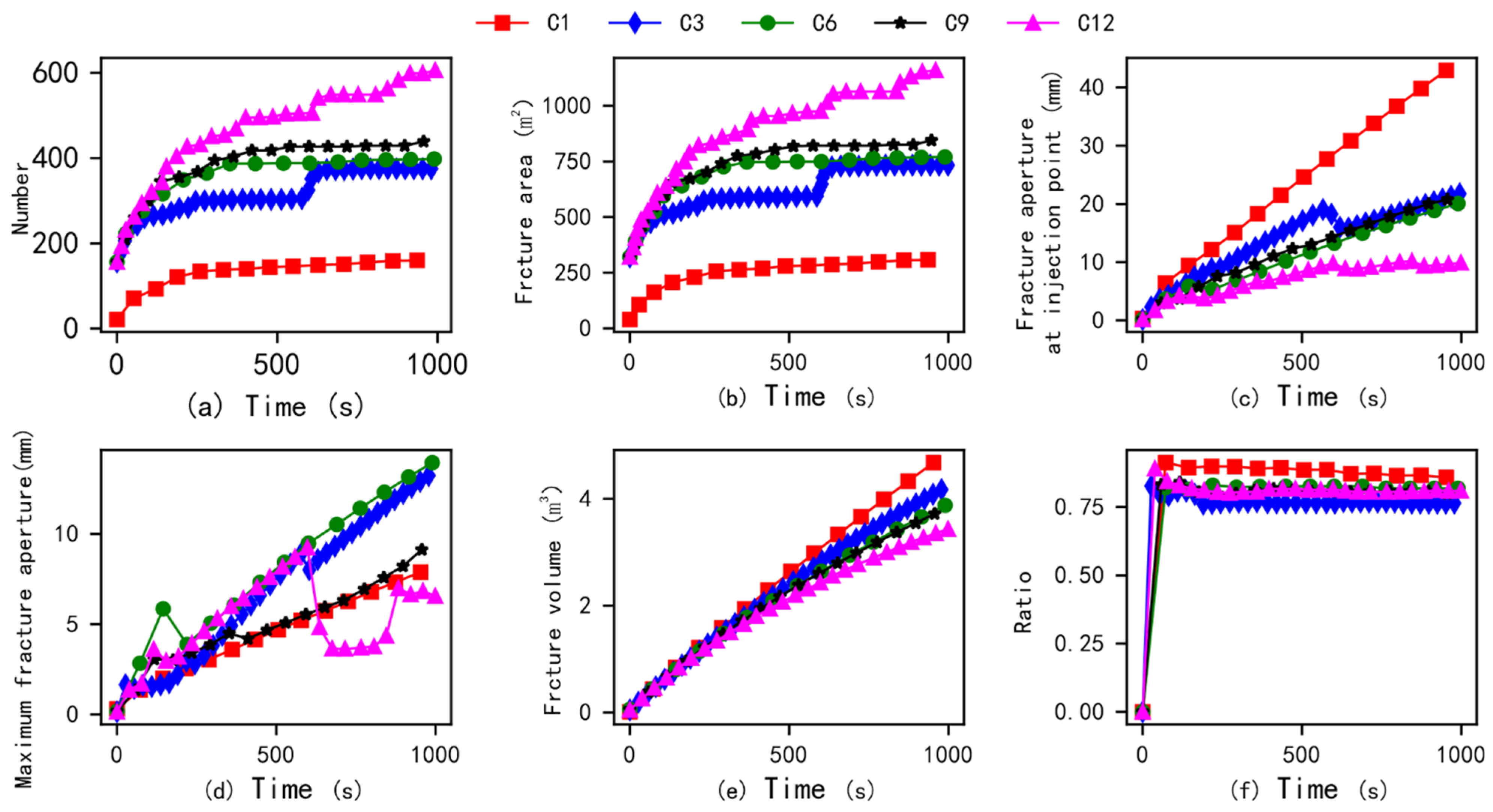
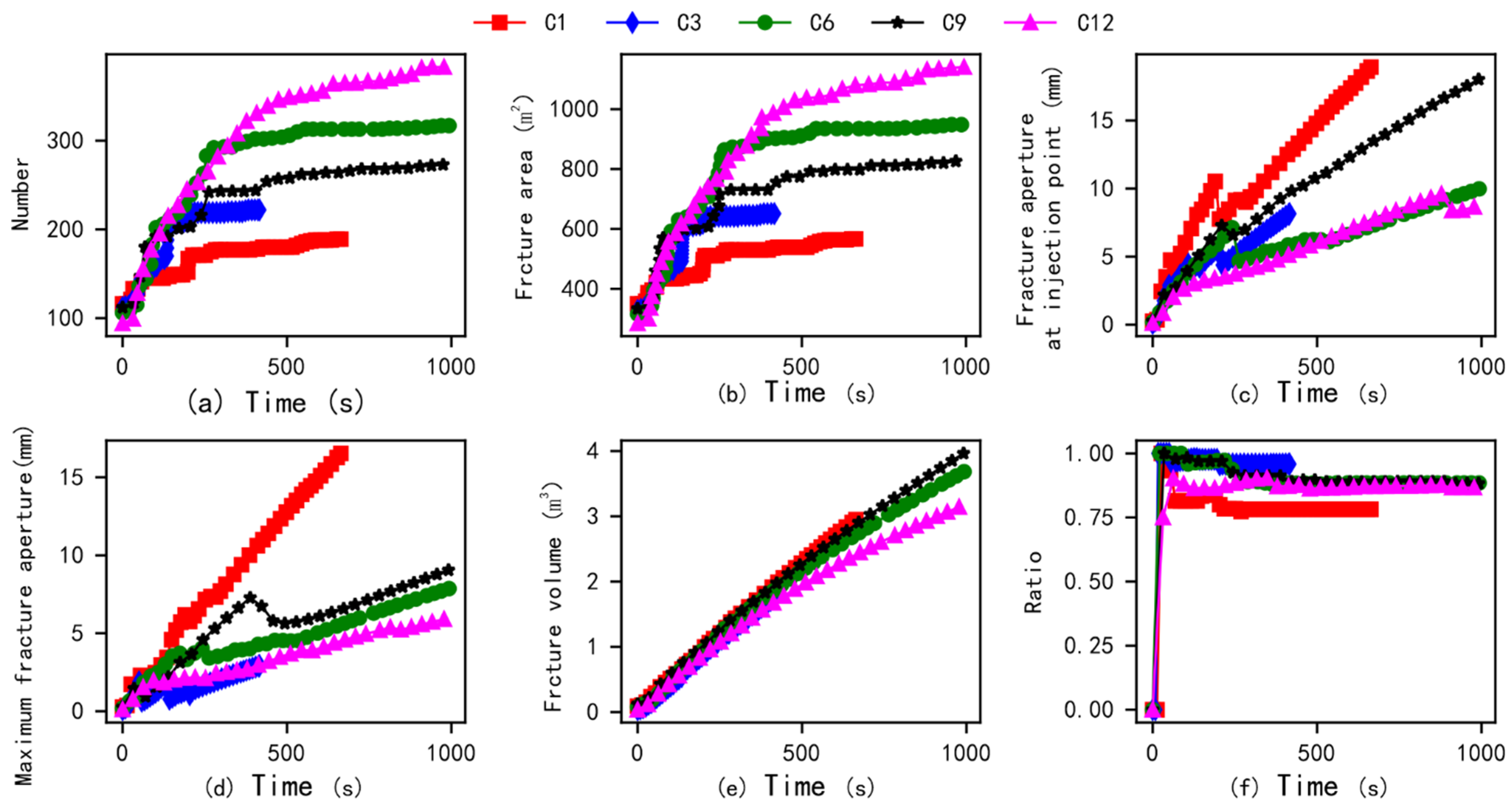
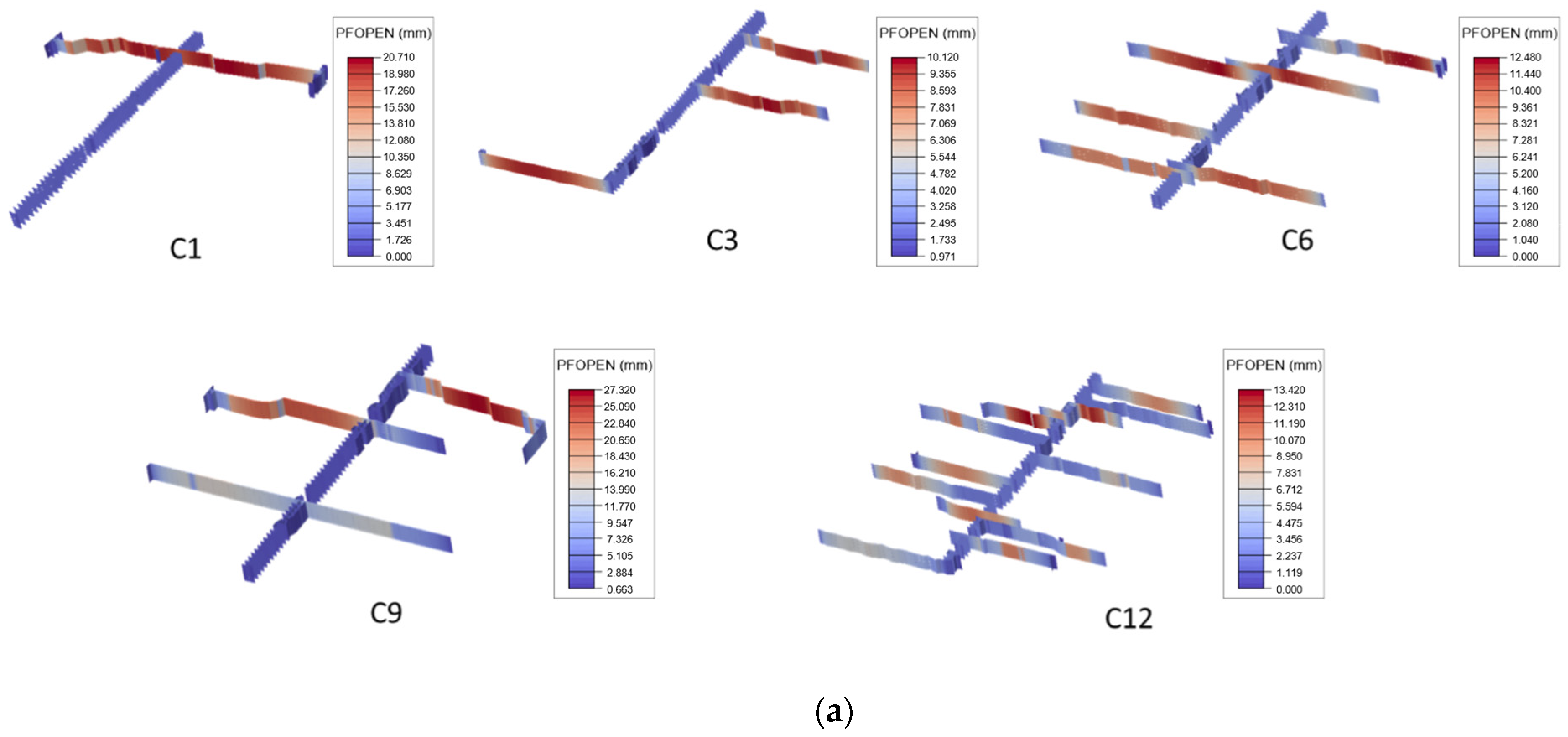
3.1. Effect of Fracturing Cluster Number

To investigate the behavior of multi-cluster fracturing under reservoir conditions in the target area, the fracture propagation results under different cluster numbers were first compared, and the results are shown in Figure 3. With inter-cluster distance increases, the fracturing simulation results of different numbers of clusters show different fracture propagation characteristics. As the number of clusters increases, the number of fracture elements and total area show an increasing trend. However, from single-cluster fracturing to triple-cluster fracturing, the increase in the number and area of fractures is relatively small. This indicates that as the number of clusters increases, the propagation of fractures is influenced by inter-cluster interactions. Concurrently, as the inter-cluster distance increases and the number of clusters is augmented, a reduction in fracture volume is observed. Intriguingly, the proportion of tensile failure within the fracture network shows a significant increase. This phenomenon suggests that single-cluster fracturing faces challenges in creating large-scale fractures. The injected fluid is primarily used to create and lengthen fractures. In contrast, multi-cluster fracturing facilitates the development of a more intricate fracture network and enhances the overall fracture volume. These observations underscore the influence of cluster configuration on fracture morphology and highlight the potential benefits of using multi-cluster fracturing strategies to optimize reservoir stimulation and enhance hydrocarbon recovery.

At a simulation time of 1000 s, the ultimate distribution of fractures is illustrated in Figure 4. It is noteworthy that as the number of clusters rises, the spacing between clusters diminishes within the model. Consequently, the total surface area covered by the induced fractures amplifies, whereas the aperture of fractures emanating from the injection point decreases. This finding indicates that with an increasing number of fracturing clusters, the area of medium-pressure fractures in the reservoir expands. However, as the total injection volume remains constant, there is a slight decreasing trend observed in the fracture aperture. Furthermore, the total volume of visible fractures decreases. These observations suggest that variations in the number of clusters and cluster spacing influence fracture morphology. The model tends to produce a higher quantity of smaller fractures influenced by a combination of factors including the model mesh, the presence of natural fractures, the number of fracturing clusters, and geo-stress conditions. This leads to an increase in the total fracture surface area and a reduction in the visible fracture volume. This behavior highlights the complex interplay between fracturing parameters and the resulting fracture network geometry.

Figure 5 presents a comparative analysis of the final morphology of artificial fractures generated under varying cluster configurations, including different numbers of clusters and cluster spacing. In single-cluster fracturing, a single dominant fracture is mainly formed, with limited fracture initiation and propagation in the near-wellbore region. However, as the number of clusters is increased to three, three primary fractures are observed to develop, exhibiting both single-wing and double-wing propagation. This suggests that increasing the number of clusters can stimulate the formation of fractures near the wellbore and facilitate the development of multiple main fractures, enhancing the overall fracture complexity. When using six clusters of fracturing, multiple fractures appeared near the wellbore. When the number of clusters increases to nine, more fractures initiate simultaneously. It is worth noting that the fracture morphology was magnified 10 times in the simulation results to observe most of the artificial fractures. However, the main path of the fractures in cluster 6 fracturing is more obvious, while cluster 9 fracturing shows a discontinuous main path, indicating the presence of many locally small opening fractures, which is not conducive to the transportation of proppants and subsequent mining. More than 12 artificial fractures have sprouted in the near-wellbore area of 12-cluster fracturing. As the fracturing process progresses, competition expands, causing some of the newly formed fractures to not open further, ultimately leading to the expansion of 10 main fractures. The above results indicate that the more fracturing clusters there are, the smaller the cluster spacing, which usually significantly increases the volume of artificial fractures, thereby improving the effectiveness of reservoir transformation. Similar conclusions can also be observed in some studies on on-site earthquake monitoring methods [37,38,39,40,41]. For example, Chen et al. found through micro seismic monitoring of shale gas reservoirs in the southwestern region that an increase in the number of fracturing clusters can promote the occurrence of more micro seismic events, and micro seismic event points near the wellbore gradually gather to form multiple bands, indicating the possibility of producing more artificial fractures. At the same time, they also found that under the influence of natural fractures and other factors, many micro seismic events may occur in areas far from the wellbore, which is significant in the expansion results of the fracturing of a single cluster in Figure 5. It is worth mentioning that compared to the 3D view, only a portion of the main seam shape is observed in the top view. This is obviously due to some fractures opening too little. Therefore, increasing the number of clusters does not necessarily lead to a proportional increase in the number of main fractures. It is crucial to consider the influence of proppant size on the effective number of supported fractures. Proppant size plays a significant role in determining the aperture and conductivity of the fractures, which ultimately affects the overall effectiveness of the fracturing treatment. By optimizing the proppant size according to the reservoir and fracturing conditions, it is possible to maximize the number of fractures effectively supported and enhance hydrocarbon recovery.

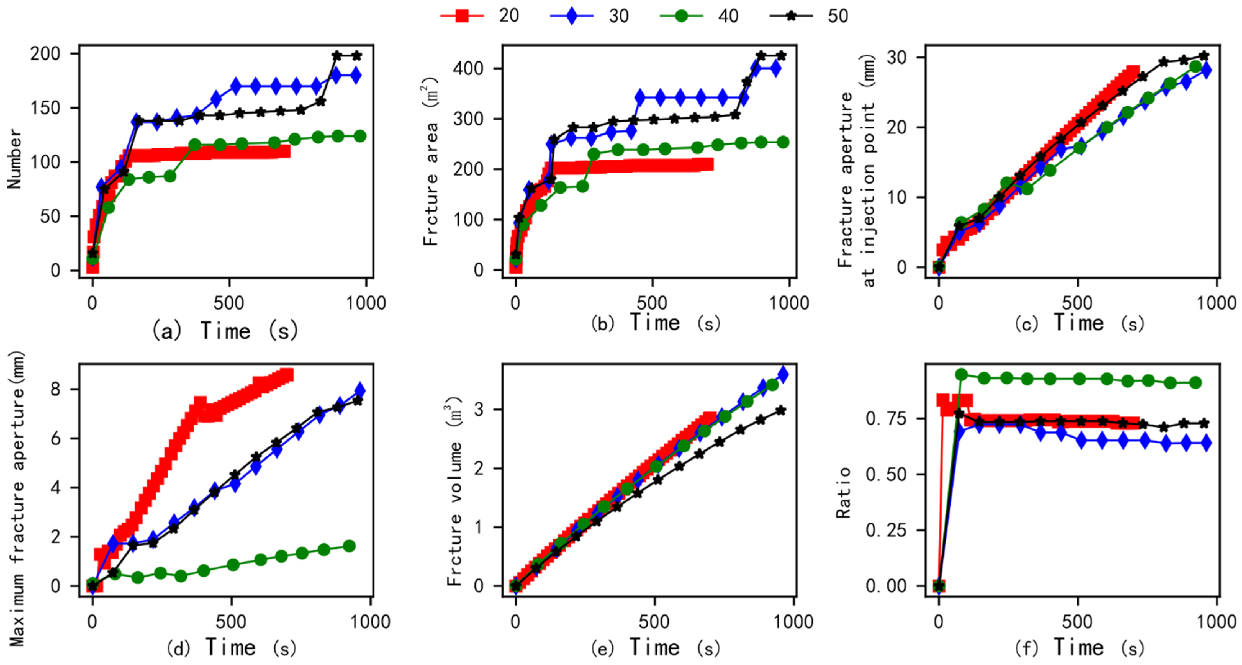
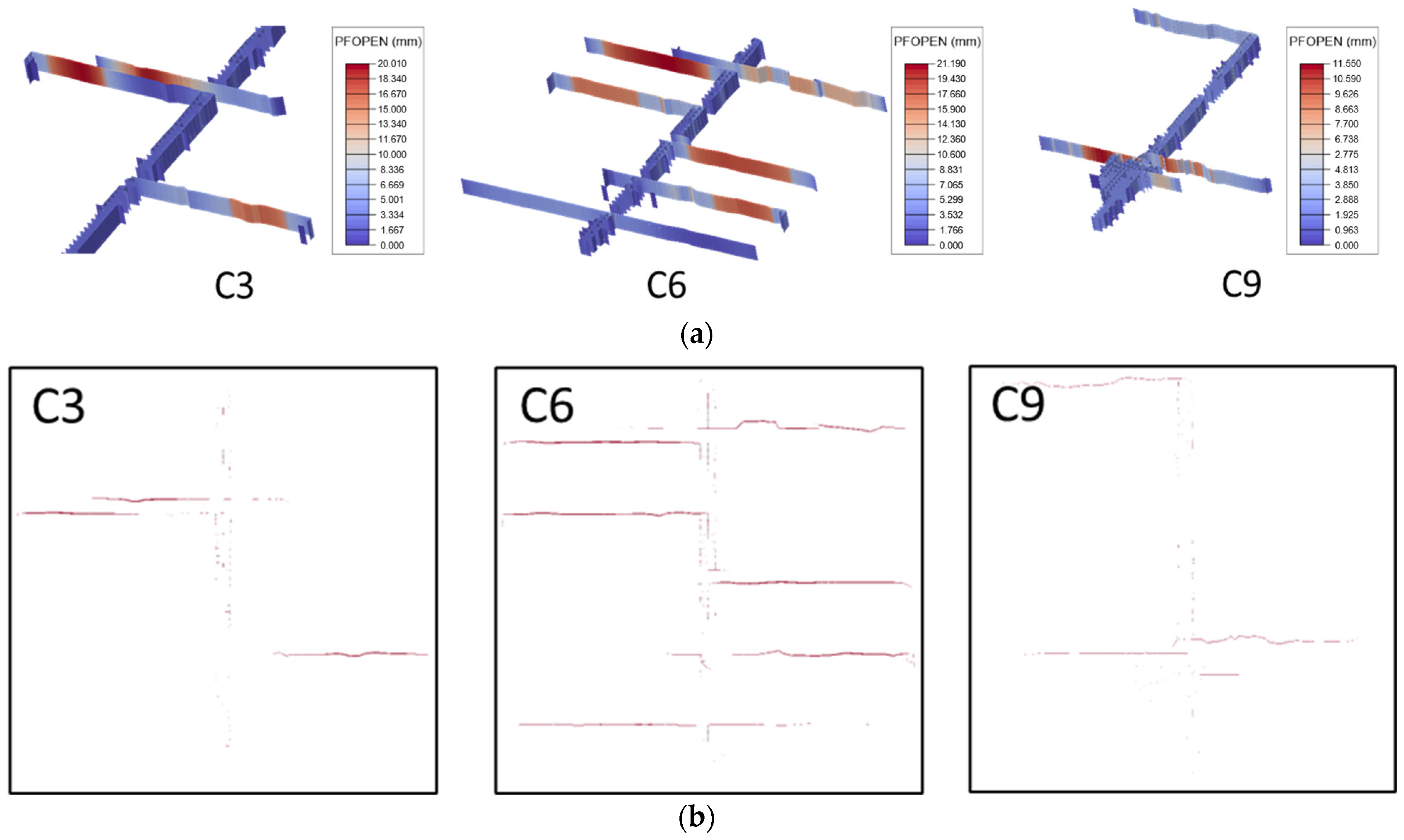
3.2. Effect of Number of Natural Fractures

The distribution of natural fractures plays a crucial role in influencing fracturing effectiveness within reservoirs. Therefore, this section undertook a simulation analysis to investigate the impact of varying numbers of natural fractures in the simulated target block. Based on the field data obtained from the target block, the linear density of natural fractures within the block falls approximately within the range from 0.3 to 0.8. Considering a simulated area of 60 m × 60 m, the number of natural fractures in the model varies from 20 to 50. The simulation results obtained are shown in Figure 6.

Figure 6 shows that with the increase in fracture density, the number of fracture elements and the total area of fractures show an increasing trend. Meanwhile, the aperture and volume of fractures seem to show a certain decreasing trend. This may be due to the increased density of natural fractures, which makes reservoir fracturing more susceptible to the influence of fractures, resulting in the formation of many low-opening shear fractures. Therefore, with the increase in natural fractures, the shear fractures generated by shear stimulation significantly increase, and the fracture area increases. At the same time, since shear fractures are mostly low-opening fractures, the visible volume of artificial fractures shows a certain fluctuation and decreasing trend.

Figure 7 illustrates the opening of artificial fractures in reservoirs under the influence of varying natural fracture densities. As depicted in the figure, with the increase in natural fractures, the number of artificial fractures in the reservoir significantly increases, and more branches and extensions of artificial fractures occur. Simultaneously, an increase in natural fractures leads to a higher likelihood of large openings in artificial fractures near the reservoir wellbore. In addition, when the number of natural fractures increases to a certain extent, it may induce single-cluster fracturing to form a multi-cluster extended artificial fracture network. The above results indicate that natural fractures have a significant impact on the development of artificial fractures during reservoir fracturing, which may alter the position of the main fractures, the distribution of fractures near the wellbore, and the bending and branching morphology of the main fractures, thereby inducing the formation of complex fracture networks and improving the effectiveness of reservoir fracturing.

3.3. Comprehensive Impact Analysis

The previous research results indicate that both the number of fracturing clusters and the number of natural fractures significantly affect the propagation pattern of artificial fractures in reservoirs [26,27]. Among them, the number of natural fractures is usually the internal condition of the reservoir, which is difficult to change through construction methods, while the number of fracturing clusters is a construction method that can be directly adjusted during on-site construction. If different cluster fracturing is used for areas with different natural fractures, it may further enhance the effectiveness of reservoir transformation. Therefore, to further discuss the comprehensive impact of multi-cluster fracturing construction and natural fractures, this section comprehensively compares and simulates the expansion of multi-cluster fracturing fractures in target reservoir areas with different numbers of natural fractures.

In Figure 8, there is a phenomenon of incomplete calculation in the fracturing results of six clusters. Therefore, the analysis is only based on the fracturing results of three and nine clusters. From the above figure, when the fracture density is 20, multi-cluster fracturing does not necessarily increase the area of reservoir fractures but has a significant impact on the volume of reservoir fractures. This phenomenon refers to the different behavior of artificial fractures within the reservoir caused by the presence of natural fractures. Notably, the presence of natural fractures often leads to a further increase in the stimulated reservoir volume (SRV). This observation highlights the importance of considering the interplay between natural fractures and hydraulic fracturing operations.

It can be significantly observed from Figure 9 that in this simulation model, there were three main fracture extensions in three clusters of fracturing, six main fracture extensions in six clusters of fracturing, and two main fractures and local complex fracture network extensions in nine clusters of fracturing. This result suggests that with an increasing number of fracturing clusters, complex fracture networks are more likely to form in the reservoir. Meanwhile, it is not difficult to observe from the results in the above figure that the two-dimensional view of the nine-cluster fracturing results is not significant, with many low-opening fractures. When considering fracture opening, the fracturing results of cluster 6 are significantly better than those of cluster 3 and cluster 9.

Figure 10 presents comparative results of traditional quantitative metrics across various cluster configurations in the presence of 30 significant natural fractures within the region of interest. Compared to the simulation results with a fracture density of 20, the simulations of 1, 3, 6, 9, and 12 clusters were all fully calculated with a fracture density of 30. Therefore, the results for different clusters with a fracture density of 30 were further extracted. From the above figure, as the number of fracturing clusters increases, the artificial fracture area, fracture opening, and shear failure ratio of the reservoir all significantly increase.

The process of fracture morphology changes when the fracture number is 30 is shown in Figure 11. As the number of fracturing clusters increases, the main artificial fractures in the reservoir show an increasing trend. Unfortunately, when fracturing 1 cluster, 1 main fracture was formed, when fracturing 3 clusters, 3 main fractures were formed, when fracturing 6 clusters, 6 main fractures were formed, and when fracturing 12 clusters, 12 main fractures were formed. However, when fracturing nine clusters, only three main fractures were formed. We speculate that this is due to the large number of fractures near the wellbore generated in the simulation model of nine-cluster fracturing, indicating that implementing nine-cluster fracturing under the conditions of this model will make it difficult to achieve economic fracturing effects.

Figure 12 presents a comparative analysis of conventional quantitative metrics across different cluster configurations in the presence of 40 natural fractures within the region of interest. In comparison to the simulation results obtained at a fracture density of 20, comprehensive simulations were conducted for 1 cluster, 3 clusters, 6 clusters, 9 clusters, and 12 clusters at a fracture density of 40. A thorough comparison was then performed on the conventional quantization parameters for various cluster configurations. As evident from the graphical representation of the results, the artificial fracture area, fracture aperture, and shear failure ratio within the reservoir all exhibit a noticeable upward trend with an increasing number of fracturing clusters. These observations highlight the significant influence of cluster configuration on fracture development and provide valuable insights for optimizing fracturing strategies to enhance reservoir stimulation and hydrocarbon recovery.

Figure 13 illustrates the evolution of fracture morphology with varying fracturing cluster configurations at a fracture density of 40. As shown in the figure, the quantity of primary artificial fractures within the reservoir progressively increases as the number of fracturing clusters grows. This observation highlights the influence of cluster configuration on fracture development and the potential for optimizing fracturing strategies to enhance reservoir stimulation and hydrocarbon recovery. Among them, there was a phenomenon of multiple main fractures branching out during the fracturing of cluster 1, indicating that fracturing a single cluster may also create a local artificial network of main fractures. When fracturing three clusters, five main fractures were formed. When the expansion degree of the main fractures decreased, 5 main fractures were formed when fracturing 6 clusters, 3 main fractures and a local fracture network expansion area were formed when fracturing 9 clusters, and 12 main fractures were formed when fracturing 12 clusters. The results indicate that as the number of fracturing clusters increases, the number of artificial main fractures increases. It is worth mentioning that previous research results have shown that as the density of natural fractures increases, artificial fractures may exhibit more bending, branching, and other expansion phenomena, forming a complex network of fractures [42,43]. Comparing the simulation results under different numbers of natural fractures and clusters in this section, as the number of natural fractures increases, artificial fractures may become more complex. For example, when the simulated target block contains 40 natural fractures, even under single-cluster fracturing conditions, more complex fracture shapes are formed. Meanwhile, when the simulated target block contains 20 natural fractures, even under the conditions of fracturing of nine clusters, it may be difficult to form a complex artificial fracture network.

4. Conclusions

Based on the FDEM and on-site data from a certain well block in Southwest China, multiple cluster fracturing simulation models were established considering the natural fractures and geological mechanical parameters of the target block. The changes in artificial fracture area, fracture aperture, fracture volume, fluid pressure, and fracture morphology in the simulation results are extracted, and the impact of the number of fracturing clusters and the number of natural fractures in the target block on the formation of artificial fractures was analyzed. The main conclusions are as follows:

(1)

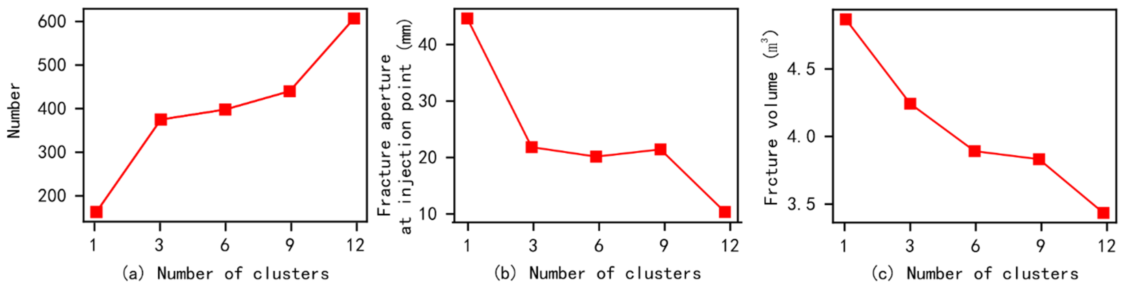
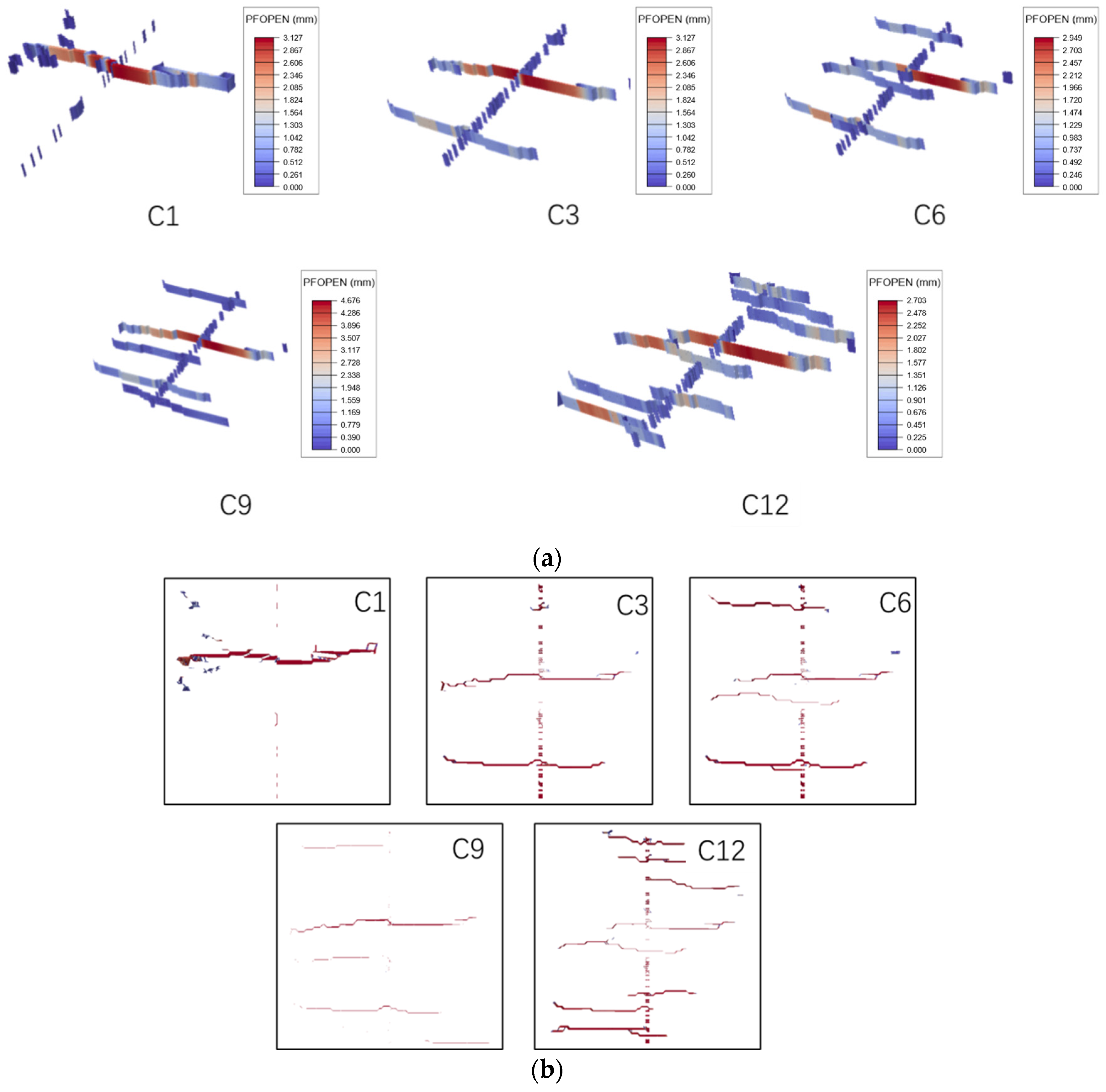
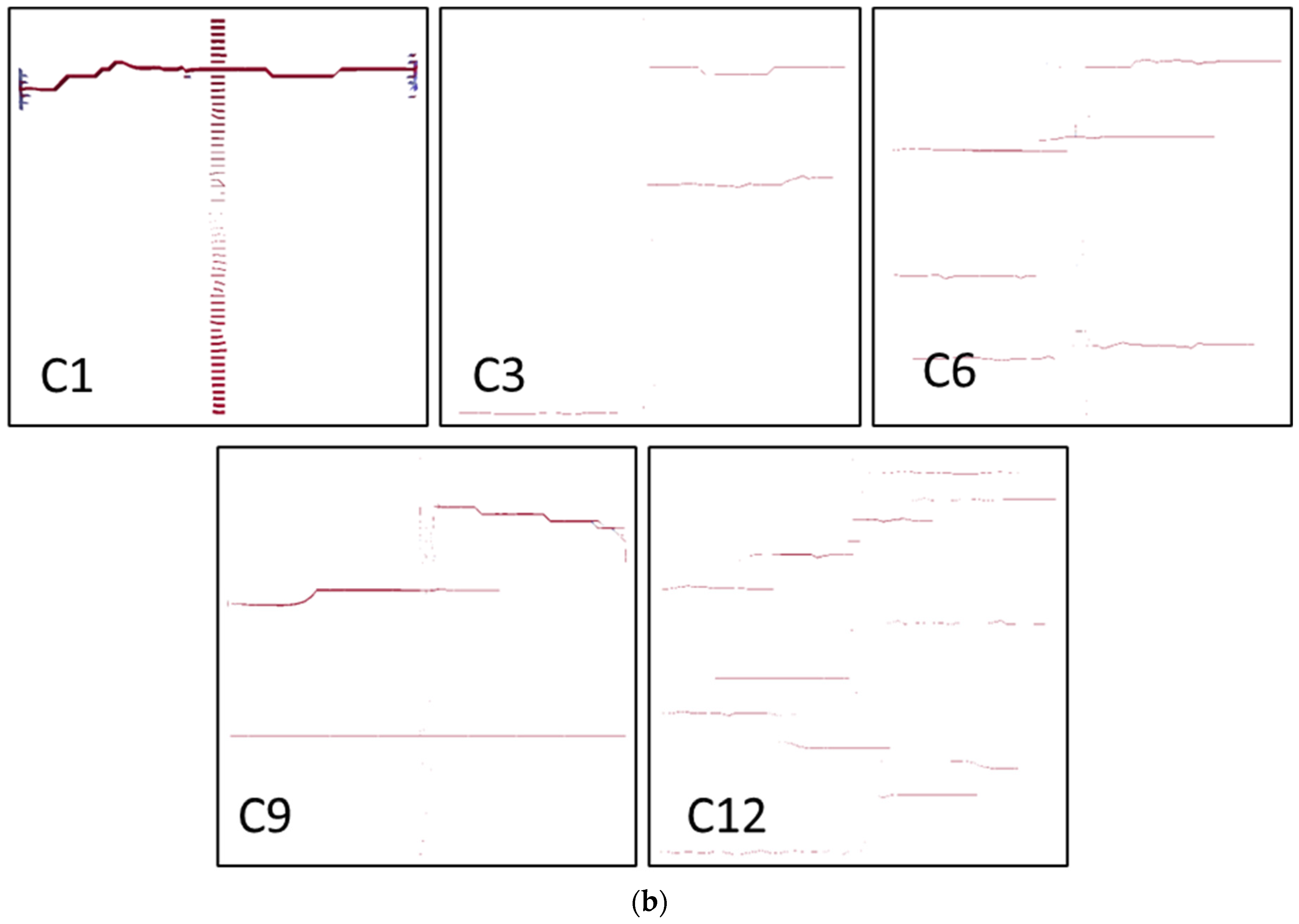
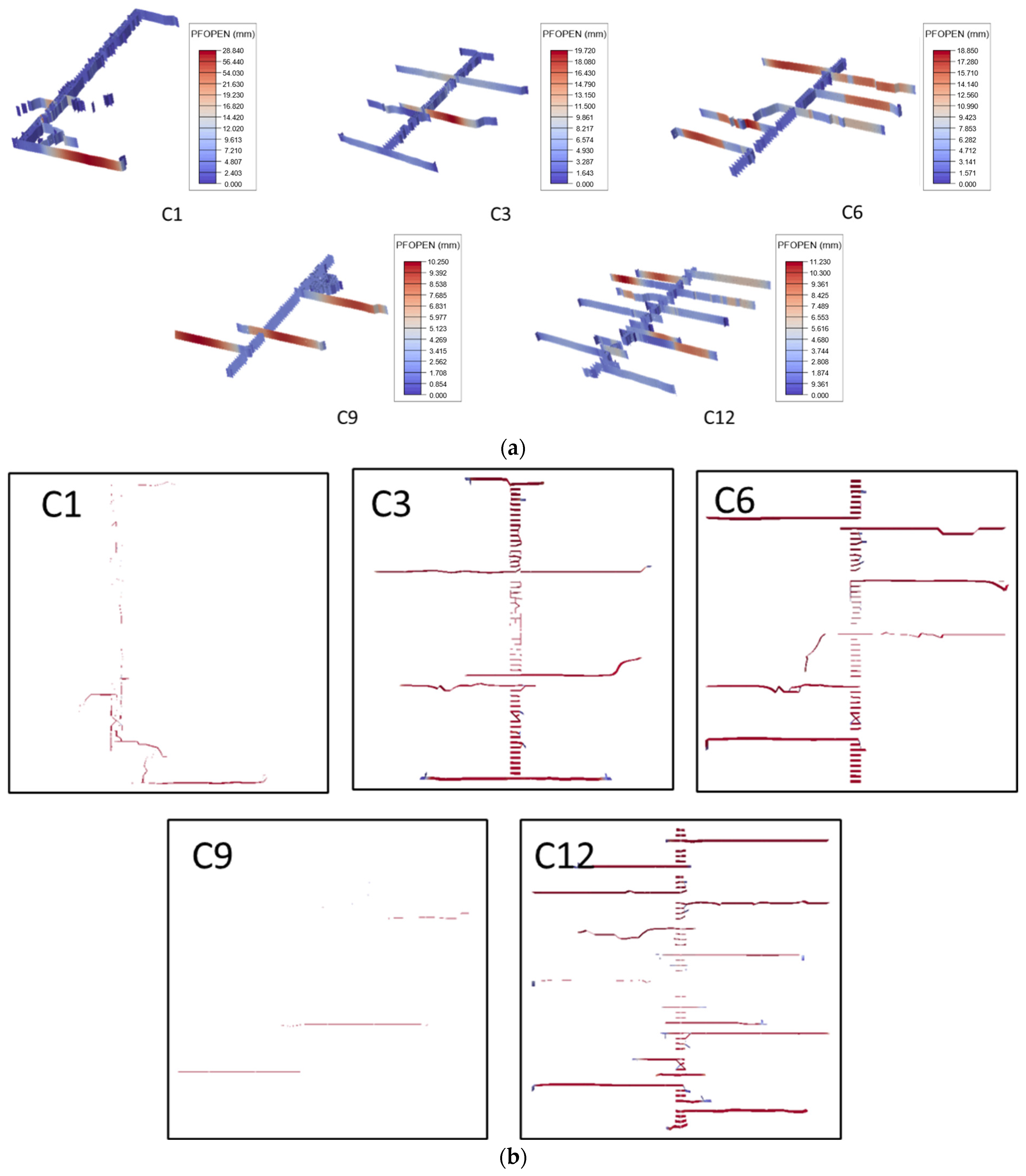
As the number of fracturing clusters increases, the number of artificial main fractures formed in the target block shows a significant increasing trend. However, when affected by the distribution of natural fractures, geo-stress, and other factors, it may also be difficult to form multiple main fractures through multi-cluster fracturing in the target block (Figure 9). Therefore, obtaining data on the spatial location and orientation of natural fractures may be more helpful in accurately estimating the fracturing effect of the target block.

(2)

Due to the influence of the original random fracturing path and natural fractures of the reservoir, shear stimulation phenomena are prone to occur. Under these conditions, artificial fractures in the reservoir are prone to bending, branching, and other phenomena. When further affected by multiple construction methods, the artificial main fracture will be more prone to single-wing expansion rather than double-wing expansion.

(3)

Multi-cluster fracturing construction may promote an increase in artificial fracture networks, but under the same injection amount, the aperture of artificial fractures will decrease. Therefore, increasing the injection rate appropriately during multi-cluster construction will be more conducive to the pumping of proppants and other materials.

(4)

The increase in the number of natural fractures in the target block will help to obtain a more complex artificial fracture network. When the number of natural fractures reaches a certain threshold, even using a single-cluster fracturing construction process may form an artificial fracture network connected by multiple main fractures.

References

1. Wu, M.; Liu, J.; Lv, X.; Shi, D.; Zhu, Z. A study on homogenization equations of fractal porous media. J. Geophys. Eng. 2018, 15, 2388–2398. [Google Scholar] [CrossRef]
2. Zheng, Y.; He, R.; Huang, L.; Bai, Y.; Wang, C.; Chen, W.; Wang, W. Exploring the effect of engineering parameters on the penetration of hydraulic fractures through bedding planes in different propagation regimes. Comput. Geotech. 2022, 146, 104736. [Google Scholar] [CrossRef]
3. Liu, Q.; Li, J.; Liang, B.; Liu, J.; Sun, W.; He, J.; Lei, Y. Complex wettability behavior triggering mechanism on imbibition: A model construction and comparative study based on analysis at multiple scales. Energy 2023, 275, 127434. [Google Scholar] [CrossRef]
4. Song, R.; Liu, J.; Cui, M. A new method to reconstruct structured mesh model from micro-computed tomography images of porous media and its application. Int. J. Heat Mass Transf. 2017, 109, 705–715. [Google Scholar] [CrossRef]
5. Wang, L.; Zhou, J.; Guo, Y.; Song, X.; Guo, W. Laboratory investigation and evaluation of the hydraulic fracturing of marine shale considering multiple geological and engineering factors. Front. Earth Sci. 2022, 10, 952655. [Google Scholar] [CrossRef]
6. Zhang, H.; Chen, J.; Li, Z.; Hu, H.; Mei, Y. Numerical Simulation of Multi-cluster Fracturing Using the Triaxiality Dependent Cohesive Zone Model in a Shale Reservoir with Mineral Heterogeneity. Rock Mech. Rock Eng. 2023, 57, 325–349. [Google Scholar] [CrossRef]
7. Nguyen, H.T.; Lee, J.H.; Elraies, K.A. A review of PKN-type modeling of hydraulic fractures. J. Pet. Sci. Eng. 2020, 195, 107607. [Google Scholar] [CrossRef]
8. Yew, C.H.; Weng, X. Chapter 1—Fracturing of a wellbore and 2D fracture models. In Mechanics of Hydraulic Fracturing, 2nd ed.; Gulf Professional Publishing: Boston, MA, USA, 2015; pp. 1–22. [Google Scholar]
9. Dontsov, E.V.; Peirce, A.P. Proppant transport in hydraulic fracturing: Crack tip screen-out in KGD and P3D models. Int. J. Solids Struct. 2015, 63, 206–218. [Google Scholar] [CrossRef]
10. Santillán, D.; Juanes, R.; Cueto-Felgueroso, L. Phase field model of fluid-driven fracture in elastic media: Immersed-fracture formulation and validation with analytical solutions. J. Geophys. Res. Solid Earth 2017, 122, 2565–2589. [Google Scholar] [CrossRef]
11. Song, R.; Liu, J.; Yang, C.; Sun, S. Study on the multiphase heat and mass transfer mechanism in the dissociation of methane hydrate in reconstructed real-shape porous sediments. Energy 2022, 254, 124421. [Google Scholar] [CrossRef]
12. Song, R.; Wang, Y.; Ishutov, S.; Zambrano-Narvaez, G.; Hodder, K.J.; Chalaturnyk, R.J.; Sun, S.; Liu, J.; Gamage, R.P. A Comprehensive Experimental Study on Mechanical Behavior, Microstructure and Transport Properties of 3D-printed Rock Analogs. Rock Mech. Rock Eng. 2020, 53, 5745–5765. [Google Scholar] [CrossRef]
13. Guo, C.; Xu, J.; Wei, M.; Jiang, R. Experimental study and numerical simulation of hydraulic fracturing tight sandstone reservoirs. Fuel 2015, 159, 334–344. [Google Scholar] [CrossRef]
14. Moghadasi, R.; Rostami, A.; Hemmati-Sarapardeh, A. Application of nanofluids for treating fines migration during hydraulic fracturing: Experimental study and mechanistic understanding. Adv. Geo-Energy Res. 2019, 3, 100–111. [Google Scholar] [CrossRef]
15. Yang, R.; Wang, Y.; Song, G.; Shi, Y. Fracturing and thermal extraction optimization methods in enhanced geothermal systems. Adv. Geo-Energy Res. 2023, 8, 136–140. [Google Scholar] [CrossRef]
16. Chen, B.; Barboza, B.R.; Sun, Y.; Bai, J.; Thomas, H.R.; Dutko, M.; Cottrell, M.; Li, C. A Review of Hydraulic Fracturing Simulation. Arch. Comput. Methods Eng. 2022, 29, 1–58. [Google Scholar] [CrossRef]
17. Yuan, J.; Jiang, R.; Zhang, W. The workflow to analyze hydraulic fracture effect on hydraulic fractured horizontal well production in composite formation system. Adv. Geo-Energy Res. 2018, 2, 319–342. [Google Scholar] [CrossRef]
18. Esfandiari, M.; Pak, A. XFEM modeling of the effect of in-situ stresses on hydraulic fracture characteristics and comparison with KGD and PKN models. J. Pet. Explor. Prod. Technol. 2023, 13, 185–201. [Google Scholar] [CrossRef]
19. Huang, L.; Liu, J.; Zhang, F.; Dontsov, E.; Damjanac, B. Exploring the influence of rock inherent heterogeneity and grain size on hydraulic fracturing using discrete element modeling. Int. J. Solids Struct. 2019, 176–177, 207–220. [Google Scholar] [CrossRef]
20. Huang, L.; Liu, J.; Zhang, F.; Fu, H.; Zhu, H.; Damjanac, B. 3D lattice modeling of hydraulic fracture initiation and near-wellbore propagation for different perforation models. J. Pet. Sci. Eng. 2020, 191, 107169. [Google Scholar] [CrossRef]
21. Zhu, X.; Feng, C.; Cheng, P.; Wang, X.; Li, S. A novel three-dimensional hydraulic fracturing model based on continuum–discontinuum element method. Comput. Methods Appl. Mech. Eng. 2021, 383, 113887. [Google Scholar] [CrossRef]
22. Wu, M.; Jiang, C.; Song, R.; Liu, J.; Li, M.; Liu, B.; Shi, D.; Zhu, Z.; Deng, B. Comparative study on hydraulic fracturing using different discrete fracture network modeling: Insight from homogeneous to heterogeneity reservoirs. Eng. Fract. Mech. 2023, 284, 109274. [Google Scholar] [CrossRef]
23. Huang, L.; Dontsov, E.; Fu, H.; Lei, Y.; Weng, D.; Zhang, F. Hydraulic fracture height growth in layered rocks: Perspective from DEM simulation of different propagation regimes. Int. J. Solids Struct. 2022, 238, 111395. [Google Scholar] [CrossRef]
24. Huang, L.; Tan, J.; Fu, H.; Liu, J.; Chen, X.; Liao, X.; Wang, X.; Wang, C. The non-plane initiation and propagation mechanism of multiple hydraulic fractures in tight reservoirs considering stress shadow effects. Eng. Fract. Mech. 2023, 292, 109570. [Google Scholar] [CrossRef]
25. Wu, M.; Zhang, D.M.; Wang, W.S.; Li, M.H.; Liu, S.M.; Lu, J.; Gao, H. Numerical simulation of hydraulic fracturing based on two-dimensional surface fracture morphology reconstruction and combined finite-discrete element method. J. Nat. Gas Sci. Eng. 2020, 82, 103479. [Google Scholar] [CrossRef]
26. Wu, M.; Wang, W.; Zhang, D.; Deng, B.; Liu, S.; Lu, J.; Luo, Y.; Zhao, W. The pixel crack reconstruction method: From fracture image to crack geological model for fracture evolution simulation. Constr. Build. Mater. 2020, 273, 121733. [Google Scholar] [CrossRef]
27. Wu, M.; Wang, W.; Song, Z.; Liu, B.; Feng, C. Exploring the influence of heterogeneity on hydraulic fracturing based on the combined finite–discrete method. Eng. Fract. Mech. 2021, 252, 107835. [Google Scholar] [CrossRef]
28. Liu, Q.; Sun, L.; Liu, P.; Chen, L. Modeling Simultaneous Multiple Fracturing Using the Combined Finite-Discrete Element Method. Geofluids 2018, 2018, 4252904. [Google Scholar] [CrossRef]
29. Rougier, E.; Munjiza, A.; Lei, Z.; Chau, V.T.; Knight, E.E.; Hunter, A.; Srinivasan, G. The combined plastic and discrete fracture deformation framework for FDEM. Int. J. Numer. Methods Eng. 2019, 121, 1020–1035. [Google Scholar] [CrossRef]
30. Yan, C.; Jiao, Y.-Y.; Zheng, H. A fully coupled three-dimensional hydro-mechanical finite discrete element approach with real porous seepage for simulating 3D hydraulic fracturing. Comput. Geotech. 2018, 96, 73–89. [Google Scholar] [CrossRef]
31. Wu, Z.; Sun, H.; Wong, L.N.Y. A Cohesive Element-Based Numerical Manifold Method for Hydraulic Fracturing Modelling with Voronoi Grains. Rock Mech. Rock Eng. 2019, 52, 2335–2359. [Google Scholar] [CrossRef]
32. Wu, M.; Gao, K.; Liu, J.; Song, Z.; Huang, X. Influence of rock heterogeneity on hydraulic fracturing: A parametric study using the combined finite-discrete element method. Int. J. Solids Struct. 2022, 234–235, 111293. [Google Scholar] [CrossRef]
33. Wu, Z.; Xu, X.; Liu, Q.; Yang, Y. A zero-thickness cohesive element-based numerical manifold method for rock mechanical behavior with micro-Voronoi grains. Eng. Anal. Bound. Elem. 2018, 96, 94–108. [Google Scholar] [CrossRef]
34. Sharafisafa, M.; Aliabadian, Z.; Sato, A.; Shen, L. Combined finite-discrete element modelling of hydraulic fracturing in reservoirs with filled joints. Geoenergy Sci. Eng. 2023, 228, 212025. [Google Scholar] [CrossRef]
35. Shi, F.; Wang, D.; Li, H. An XFEM-based approach for 3D hydraulic fracturing simulation considering crack front segmentation. J. Pet. Sci. Eng. 2022, 214, 110518. [Google Scholar] [CrossRef]
36. Cramer, D.; Friehauf, K.; Roberts, G.; Whittaker, J. Integrating DAS, Treatment Pressure Analysis and Video-Based Perforation Imaging to Evaluate Limited Entry Treatment Effectiveness. In Proceedings of the SPE Hydraulic Fracturing Technology Conference and Exhibition, The Woodlands, TX, USA, 5–7 February 2019; p. D031S007R001. [Google Scholar]
37. Chen, H.; Meng, X.; Niu, F.; Tang, Y.; Yin, C.; Wu, F. Microseismic Monitoring of Stimulating Shale Gas Reservoir in SW China: 2. Spatial Clustering Controlled by the Preexisting Faults and Fractures. J. Geophys. Res. Solid Earth 2018, 123, 1659–1672. [Google Scholar] [CrossRef]
38. Ou, C.; Liang, C.; Li, Z.; Luo, L.; Yang, X. 3D visualization of hydraulic fractures using micro-seismic monitoring: Methodology and application. Petroleum 2022, 8, 92–101. [Google Scholar] [CrossRef]
39. Lu, Z.; Jia, Y.; Cheng, L.; Pan, Z.; Xu, L.; He, P.; Guo, X.; Ouyang, L. Microseismic Monitoring of Hydraulic Fracture Propagation and Seismic Risks in Shale Reservoir with a Steep Dip Angle. Nat. Resour. Res. 2022, 31, 2973–2993. [Google Scholar]
40. Shang, X.; Long, S.; Duan, T. Fracture system in shale gas reservoir: Prospect of characterization and modeling techniques. J. Nat. Gas Geosci. 2021, 6, 157–172. [Google Scholar] [CrossRef]
41. Li, Y.; Cheng, C.H.; Toksöz, M.N. Seismic monitoring of the growth of a hydraulic fracture zone at Fenton Hill, New Mexico. Geophysics 1998, 63, 120–131. [Google Scholar] [CrossRef]
42. Dahi Taleghani, A.; Gonzalez-Chavez, M.; Yu, H.; Asala, H. Numerical simulation of hydraulic fracture propagation in naturally fractured formations using the cohesive zone model. J. Pet. Sci. Eng. 2018, 165, 42–57. [Google Scholar] [CrossRef]
43. Wang, H. Hydraulic fracture propagation in naturally fractured reservoirs: Complex fracture or fracture networks. J. Nat. Gas Sci. Eng. 2019, 68, 102911. [Google Scholar] [CrossRef]
Figure 1. Schematic diagram of reservoir multi-cluster fracturing and FDEM principle.
Applsci 14 06342 g001
Figure 2. Schematic diagram of FDEM models with natural fractures: (a) 20 natural fractures; (b) 30 natural fractures; (c) 40 natural fractures; (d) 50 natural fractures.
Applsci 14 06342 g002
Figure 3. Results of conventional quantitative metrics under different cluster configurations ((a) number of damaged interface elements versus time; (b) fracture area versus time; (c) fracture aperture at injection point versus time; (d) maximum fracture aperture versus time; (e) fracture volume versus time; and (f) ratio of tensile failure versus time) (C1, C3, C6, C9, and C12 refer to fracturing scenarios involving 1 cluster, 3 clusters, 6 clusters, 9 clusters, and 12 clusters, respectively).
Applsci 14 06342 g003
Figure 4. Results of conventional quantization parameters ((a) number of damaged interface elements versus number of fracturing clusters; (b) fracture aperture at injection point versus number of fracturing clusters; and (c) fracture volume versus number of fracturing clusters) (1000 s).
Applsci 14 06342 g004
Figure 5. Morphology comparison results of artificial fractures under different cluster numbers ((a) 3D view and (b) top view) (C1, C3, C6, C9, and C12 refer to fracturing scenarios involving 1 cluster, 3 clusters, 6 clusters, 9 clusters, and 12 clusters, respectively).
Applsci 14 06342 g005
Figure 6. Results of conventional quantitative metrics under influence of number of natural fractures ((a) number of damaged interface elements versus time; (b) fracture area versus time; (c) fracture aperture at injection point versus time; (d) maximum fracture aperture versus time; (e) fracture volume versus time; and (f) ratio of tensile failure versus time) (numbers (20, 30, 40, 50) represent quantity of natural fractures in various simulation models).
Applsci 14 06342 g006
Figure 7. The results of the artificial fracture morphology in reservoirs under the influence of different natural fracture numbers ((a) is a 3D view and (b) is a top view) (the numbers (20, 30, 40, 50) represent the quantity of natural fractures in various simulation models).
Applsci 14 06342 g007
Figure 8. Results of conventional quantitative metrics under different cluster configurations when there are 20 natural fractures in region ((a) number of damaged interface elements versus time; (b) fracture area versus time; (c) fracture aperture at injection point versus time; (d) maximum fracture aperture versus time; (e) fracture volume versus time; and (f) ratio of tensile failure versus time) (C3, C6, and C9 correspond to fracturing scenarios involving 3 clusters, 6 clusters, and 9 clusters, respectively).
Applsci 14 06342 g008
Figure 9. Fracture morphology under diverse cluster fracturing scenarios when there are 20 natural fractures in the region ((a) is a 3D view and (b) is a top view) (C3, C6, and C9 correspond to fracturing scenarios involving 3 clusters, 6 clusters, and 9 clusters, respectively).
Applsci 14 06342 g009
Figure 10. The comparison results of conventional quantitative parameters under the influence of different clusters when there are 30 natural fractures in the region ((a) number of damaged interface elements versus time; (b) fracture area versus time; (c) fracture aperture at injection point versus time; (d) maximum fracture aperture versus time; (e) fracture volume versus time; and (f) ratio of tensile failure versus time) (C1, C3, C6, C9, and C12 represent fracturing scenarios involving 1 cluster, 3 clusters, 6 clusters, 9 clusters, and 12 clusters, respectively).
Applsci 14 06342 g010
Figure 11. Fracture morphology under diverse cluster fracturing scenarios when there are 30 natural fractures in the region ((a) is a 3D view and (b) is a top view) (C1, C3, C6, C9, and C12 represent fracturing scenarios involving 1 cluster, 3 clusters, 6 clusters, 9 clusters, and 12 clusters, respectively).
Applsci 14 06342 g011aApplsci 14 06342 g011b
Figure 12. The comparative results of conventional quantitative metrics under varying cluster configurations in the presence of 40 natural fractures within the region ((a) number of damaged interface elements versus time; (b) fracture area versus time; (c) fracture aperture at injection point versus time; (d) maximum fracture aperture versus time; (e) fracture volume versus time; and (f) ratio of tensile failure versus time) (C1, C3, C6, C9, and C12 represent fracturing scenarios involving 1 cluster, 3 clusters, 6 clusters, 9 clusters, and 12 clusters, respectively).
Applsci 14 06342 g012
Figure 13. Fracture morphology under diverse cluster fracturing scenarios when there are 40 natural fractures in the region ((a) is a 3D view and (b) is a top view) (C1, C3, C6, C9, and C12 represent fracturing scenarios involving 1 cluster, 3 clusters, 6 clusters, 9 clusters, and 12 clusters, respectively).
Applsci 14 06342 g013