A Fault Diagnosis Method for a Missile Air Data System Based on Unscented Kalman Filter and Inception V3 Methods

Abstract

Due to the complexity of the missile air data system (ADS) and the harshness of the environment in which its sensors operate, the effectiveness of traditional fault diagnosis methods is significantly reduced. To this end, this paper proposes a method fusing the model and neural network based on unscented Kalman filter (UKF) and Inception V3 to enhance fault diagnosis performance. Initially, the unscented Kalman filter model is established based on an atmospheric system model to accurately estimate normal states. Subsequently, in order to solve the difficulties such as threshold setting in existing fault diagnosis methods based on residual observers, the UKF model is combined with a neural network, where innovation and residual sequences of the UKF model are extracted as inputs for the neural network model to amplify fault characteristics. Then, multi-scale features are extracted by the Inception V3 network, combined with the efficient channel attention (ECA) mechanism to improve diagnostic results. Finally, the proposed algorithm is validated on a missile simulation platform. The results show that, compared to traditional methods, the proposed method achieves higher accuracy and maintains its lightweight nature simultaneously, which demonstrates its efficiency and potential of fault diagnosis in missile air data systems.

1. Introduction

Currently, the possession and level of development of missile weapons have become increasingly important for assessing a country’s military and technological capabilities. Within the various components of a missile system, the air data system (ADS) is primarily responsible for measuring atmospheric parameters during missile flight and calculating the relevant flight parameters required for guidance and control [1,2]. However, sensors of the ADS may experience failures due to harsh flight environments, such as unexpected impact, electromagnetic interference, and component anomalies, leading to the output of incorrect flight parameters. This may result in errors in subsequent control and guidance processes, potentially causing catastrophic accidents [3,4]. Therefore, conducting fault diagnosis for ADSs is of significant importance, which requires the timely detection and identification of faults following their occurrence and plays a crucial role in ensuring missile reliability and mission completion.

In the field of aircraft fault diagnosis, model-based approaches and data-based approaches are two main strategies presently used [5,6]. Model-based diagnostic methods generate relevant residuals through parameter estimation [7], state estimation [8], equivalent space methods [9], etc. These residuals are then used for fault diagnosis via approaches such as the chi-squared test [10,11,12,13] and optimal parity vector method [14,15,16]. However, it is challenging to establish the ADS model to some extent, and traditional residual generation methods based on atmospheric data calculation equations fail to comprehensively consider various environmental interference factors in practical situations. This often creates difficulties in distinguishing between normal and faulty conditions, resulting in decreased diagnostic accuracy. To represent fault features more clearly, Peng et al. [17] introduced an augmented fault filter into a kinematic model that includes atmospheric parameters, enabling fault detection, isolation, and estimation. However, this requires setting fault thresholds separately for each sensor, which results in a lack of adaptability. Building upon this, a dual Kalman filter with fault/no-fault states is designed in reference [18], where the occurrence of faults is judged through the different conditional probabilities of two filters allocated by their respective innovation and covariance, and this method achieves good robustness. Furthermore, references [19,20,21,22] have made improvements to model establishment and diagnostic methods in practical scenarios based on different strategies. Nevertheless, model-based approaches require complex designs to extract reliable fault characteristics, and often suffer from worse accuracy and real-time performance in the diagnostic process when relevant conditions are changeable, which restricts their application in the fault diagnosis of ADSs.

With the advancement of artificial intelligence technology, data-based methods utilized for fault diagnosis have emerged, including support vector machines [23,24] and neural networks [25,26,27]. These methods can extract fault features from large amounts of data without the need for precise models, and have achieved promising results in the field of fault diagnosis. Xu et al. [28] constructed a single-dimensional fully convolutional neural network characterized by multi channels for fault detection. This technique extracts features at various scales, capturing both local and general information of the sensor signal sequence to achieve a comprehensive and accurate classification. Xia et al. [29] developed a fault diagnosis model based on a bi-directional gated recurrent unit (GRU) and multi-layer perceptron (MLP). By combining the data attention mechanism and spatial attention mechanism, the model captures the semantic relationship between monitoring variables and faults, enabling fault detection and identification for autonomous underwater vehicles (AUVs). However, these methods rely on the support of sufficient data, and missile mission environments are complex, making it difficult to differentiate between faults and variations in flight states solely through data. Moreover, challenges still exist in diagnosing minor faults under the influence of noise and other interferences, which may result in worse performances in practical engineering applications.

Due to the inherent difficulty of accurately diagnosing faults in sensors and the unique nature of utilizing redundant information [30,31], models can be established based on the characteristics of multiple sensors. For example, various integrated navigation system models can be built with an inertial navigation system (INS) as the benchmark [32,33,34], combined with data-based strategies, such as neural networks, to achieve fault diagnosis. Zuo et al. [35] established a Kalman filter model for an electric multiple unit (EMU) braking system, which generated integrated filtering data with higher signal quality, and then the time domain parameters of the relay valve input and the output pressure signal are input into the SVM, achieving high diagnostic accuracy under small sample conditions. Nonetheless, it is still data-based in essence, and although it enhances the signal quality, it still faces difficulties in distinguishing between faults and variations in flight states through the measurement signals themselves. To overcome this challenge, one approach is to extract data from the model calculation process that can reflect fault conditions and input them into the neural network for fault diagnosis. This can effectively address the issues faced by data-based methods, because certain data calculated by the model under normal conditions exhibit sequences fluctuating around zero, while faults significantly disrupt this characteristic [36,37]. Such data are ideal input features for the neural network, which is able to significantly improve diagnostic results. Zhao et al. [38] proposed a fault diagnosis algorithm based upon long short-term memory (LSTM) for the Strapdown Inertial Navigation System (SINS)/Ultra-Short Baseline (USBL)/Doppler Velocity Log (DVL)/Depth Gauge (DG) integrated navigation system. It extracts normalized residual sequences generated by the Kalman filter model, then inputs this sequence into the LSTM network to monitor the sequences, which outperforms the traditional chi-squared detection method in respect of speed and accuracy. Such a method still has potential for improvement, yet the thought of combining models with neural networks is worth further exploration.

Building upon the aforementioned research, aiming at enhancing the diagnostic effectiveness of ADSs under changing conditions, this article proposes an innovative method based on the UKF and Inception V3. The UKF (unscented Kalman filter) is an improvement on the Kalman filter, and it has advantages in nonlinear systems due to its ability to approximate probability distributions. It is particularly suitable for complex and strongly nonlinear systems, like the ADS. Not only does the UKF model allow the estimation of the normal state, but also certain information obtained during its computation process can reflect fault characteristics effectively. The Inception model is an extension of the convolutional layer in terms of depth and width. It constructs a fundamental neural unit structure, which uses convolution or pooling operations with different scales of convolutional kernels and concatenates the features along the dimension, to build a network architecture that maintains network sparsity and high-performance computing, and Inception V3 improves upon the specific structure to further reduce parameter calculations. By combining UKF with Inception V3, the fault characteristics will be more prominent, and it compensates for the limitations of the methods of the model or data. This integration enhances the diagnostic effectiveness of ADSs for missiles in complex and dynamic environments, such as random target movements and sensor noises, thus ensuring the reliability of missile missions. The main contributions of this article are summarized as follows:

(1)

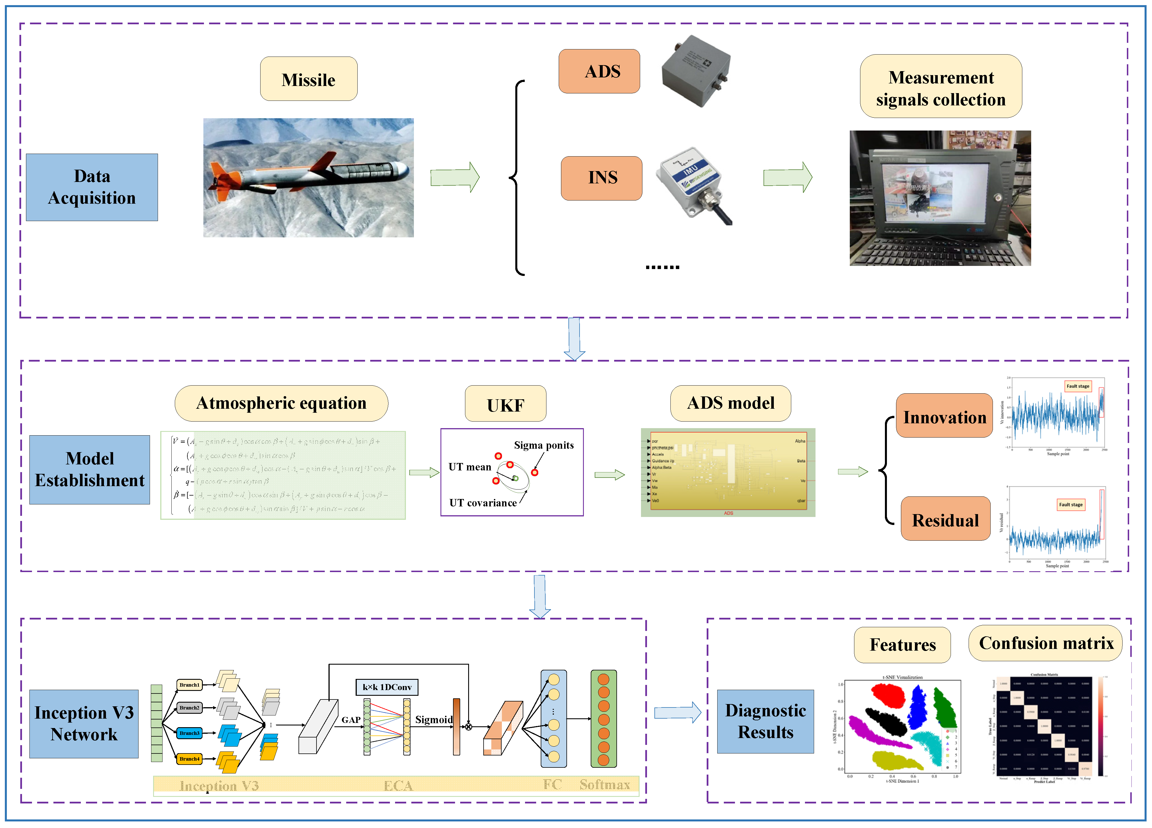
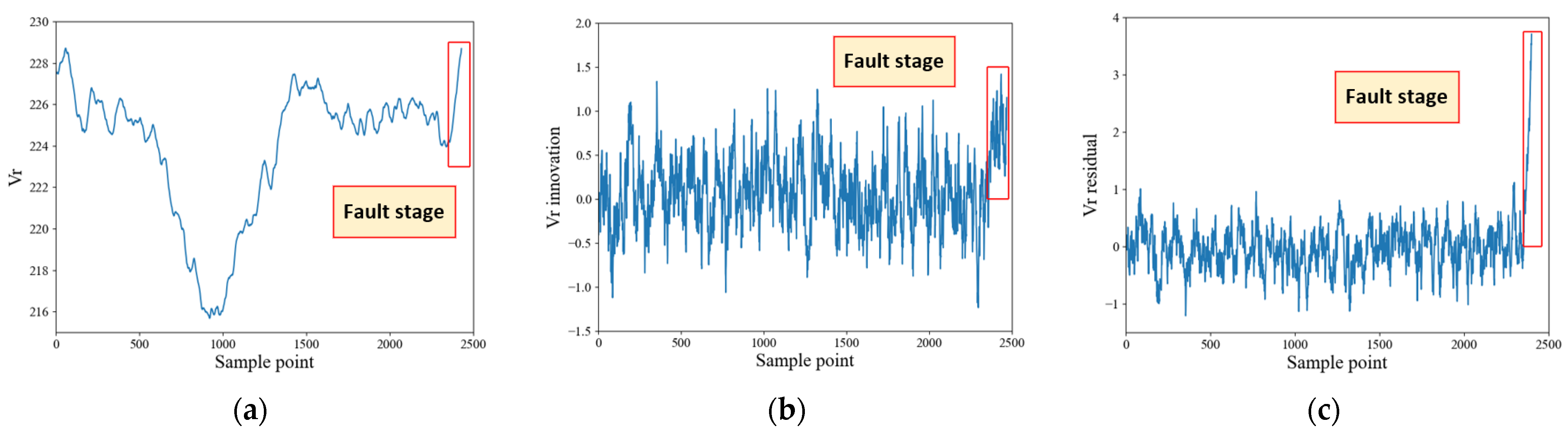
Based on the idea of integrating model and data methods, after establishing the unscented Kalman filter model for the air data system, data that reflect fault information, including innovations and residual sequences, were extracted and input into the neural network. This approach effectively overcomes the limitations of model-based and data-based methods, allowing faults to be diagnosed more easily and accurately.

(2)

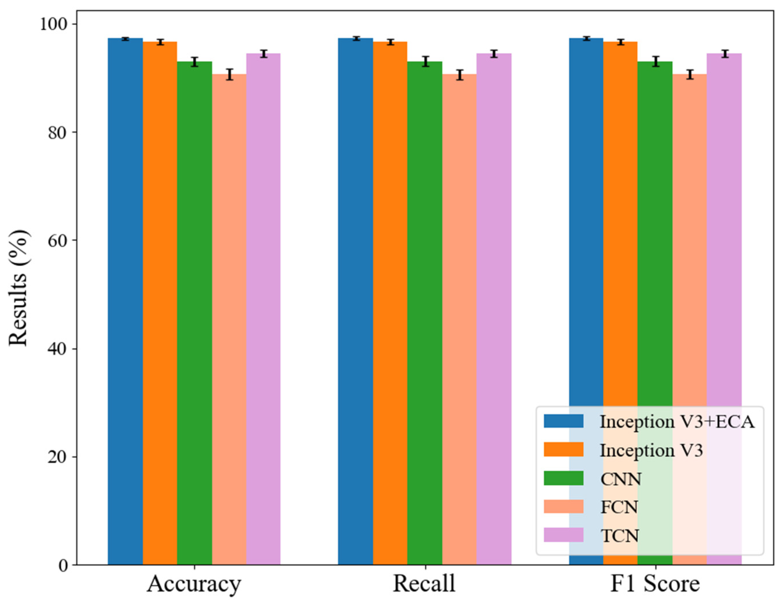
A neural network model for fault diagnosis based on Inception V3 architecture was constructed, incorporating the lightweight attention mechanism known as ECA. Compared to traditional neural networks, this network is able to learn features of data at multiple scales and in a selective manner while ensuring higher computational efficiency and requiring fewer computational resources.

The structure of this paper is arranged as follows: Section 2 introduces the model of the air data system and describes the main problems in fault diagnosis; Section 3 provides a detailed description of the proposed method; in Section 4, the experimental procedure and results are provided; and Section 5 summarizes the work of this paper.

2. Problem Description

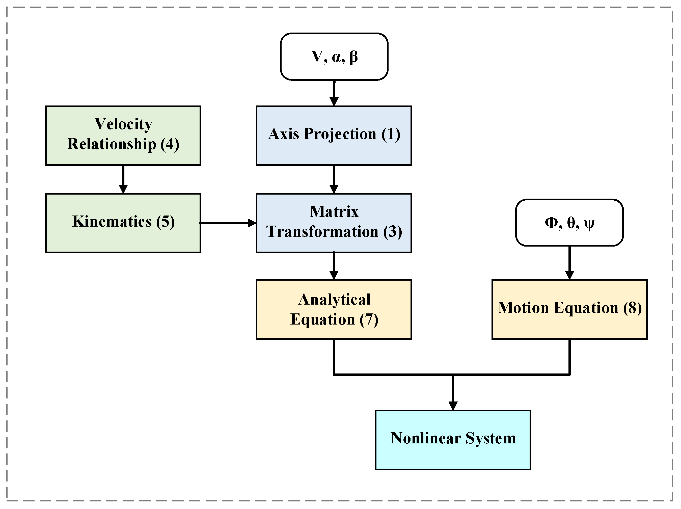
2.1. ADS Model

When establishing a model for the relevant parameters of an ADS, it is desired to unify the formula derivation in a single frame, namely the body frame, for example. In order to clarify the derivation process, Figure 1 shows the relationship between the body frame and other frames, as well as the representation of correlated parameters. The meanings of these parameters will be presented below, and the specific definitions are not elaborated upon for the sake of simplicity.

The air data system obtains measurements, such as angle of attack $\alpha$, sideslip angle $\beta$, and airspeed $V$, from its various sensors, and their interdependencies can be established by deriving the equations that describe the relationships between these measurements. Airspeed $V$ and its components in the body frame ${\left[u,v,w\right]}^{\mathrm{T}}$ can be represented as follows:

$$\left\{\begin{array}{l}u=V\cos \alpha \cos \beta \\ v=V\sin \beta \\ w=V\sin \alpha \cos \beta \end{array}\right.$$

(1)

Taking the derivative of Equation (1) yields:

$$\left\{\begin{array}{l}\stackrel{•}{u}=\stackrel{•}{V}\cos \alpha \cos \beta -\stackrel{•}{\alpha }V\sin \alpha \cos \beta -\stackrel{•}{\beta }V\cos \alpha \sin \beta \\ \stackrel{•}{v}=\stackrel{•}{V}\sin \beta +\stackrel{•}{\beta }V\cos \beta \\ \stackrel{•}{w}=\stackrel{•}{V}\sin \alpha \cos \beta +\stackrel{•}{\alpha }V\cos \alpha \cos \beta -\stackrel{•}{\beta }V\sin \alpha \sin \beta \end{array}\right.$$

(2)

After a matrix transformation, Equation (2) can be transformed into the following form:

$$\left\{\begin{array}{l}\stackrel{•}{V}=\stackrel{•}{u}\cos \alpha \cos \beta +\stackrel{•}{v}\sin \beta +\stackrel{•}{w}\sin \alpha \cos \beta \\ \stackrel{•}{\alpha }=-{\displaystyle \frac{1}{V\cos \beta }}\left(\stackrel{•}{u}\sin \alpha -\stackrel{•}{w}\cos \alpha \right)\\ \stackrel{•}{\beta }=-{\displaystyle \frac{1}{V}}\left(\stackrel{•}{u}\cos \alpha \sin \beta -\stackrel{•}{v}\cos \beta +\stackrel{•}{w}\sin \alpha \sin \beta \right)\end{array}\right.$$

(3)

Furthermore, there exists a relationship between the ground velocity vector ${\mathit{V}}_{\mathrm{e}}$, air velocity vector ${\mathit{V}}_{\mathrm{r}}$, and wind velocity vector ${\mathit{V}}_{\mathrm{w}}$:

$${\mathit{V}}_{\mathrm{e}}={\mathit{V}}_{\mathrm{r}}+{\mathit{V}}_{\mathrm{w}}$$

(4)

The kinematics equation of the missile in the body frame can be written in the following form:

$$\stackrel{•}{{\mathit{V}}_{\mathrm{e}}}=\mathit{A}+{\mathrm{T}}_{\mathrm{b}\mathrm{e}}\mathit{g}-\mathit{\omega }\times {\mathit{V}}_{\mathrm{e}}$$

(5)

where $\mathit{A}$ is the acceleration vector, $T_{be}$ is the transformation matrix from inertial frame to body from, $\mathit{g}={\left[0,0,9.81\right]}^{\mathrm{T}}$, and $\mathit{\omega }$ is the angular velocity vector.

Substituting Equation (4) into Equation (5) yields:

$$\stackrel{•}{{\mathit{V}}_{\mathrm{r}}}=\mathit{A}+T_{\mathrm{b}\mathrm{e}}\mathit{g}-\mathit{\omega }\times {\mathit{V}}_{\mathrm{r}}-\stackrel{•}{{\mathit{V}}_{\mathrm{w}}}-\mathit{\omega }\times {\mathit{V}}_{\mathrm{w}}$$

(6)

As the wind velocity is relatively small during the missile’s flight, we can denote the wind-related disturbance as $\mathit{d}$, $\mathit{d}=-\stackrel{•}{{\mathit{V}}_{\mathrm{w}}}-\mathit{\omega }\times {\mathit{V}}_{\mathrm{w}}$, then define ${\mathit{V}}_{\mathrm{r}}={\left[u,v,w\right]}^{\mathrm{T}}$, $\mathit{A}={\left[A_x,A_y,A_z\right]}^{\mathrm{T}}$, $\mathit{\omega }={\left[p,q,r\right]}^T$, and $\mathit{d}={\left[d_u,d_v,d_w\right]}^{\mathrm{T}}$. By substituting Equations (1) and (6) into Equation (3), it can be shown that:

$$\left\{\begin{array}{ll}\hfill \dot{V}=& \left(A_x-g\sin \theta +d_u\right)\cos \alpha \cos \beta +\left(A_y+g\sin \varphi \cos \theta +d_v\right)\sin \beta +\hfill \\ \hfill \hspace{1em}\hspace{1em}& \left(A_z+g\cos \varphi \cos \theta +d_w\right)\sin \alpha \cos \beta \hfill \\ \hfill \dot{\alpha }=& [\left(A_z+g\cos \varphi \cos \theta +d_w\right)\cos \alpha -\left(A_x-g\sin \theta +d_u\right)\sin \alpha ]/V\cos \beta +\hfill \\ \hfill \hspace{1em}\hspace{1em}& q-(p\cos \alpha +r\sin \alpha )\tan \beta \hfill \\ \hfill \dot{\beta }=& [-\left(A_x-g\sin \theta +d_u\right)\cos \alpha \sin \beta +\left(A_y+g\sin \varphi \cos \theta +d_v\right)\cos \beta -\hfill \\ \hfill \hspace{1em}\hspace{1em}& \left(A_z+g\cos \varphi \cos \theta +d_w\right)\sin \alpha \sin \beta ]/V+p\sin \alpha -r\cos \alpha \hfill \end{array}\right.$$

(7)

where $\varphi$, $\theta$, and $\psi$ represent the roll, pitch, and yaw angle, respectively. The estimated attitude angles can be obtained through the following set of motion equations:

$$\left\{\begin{array}{l}\dot{\varphi }=p+q\sin \varphi \tan \theta +r\cos \varphi \tan \theta \\ \dot{\theta }=q\cos \varphi -r\sin \varphi \\ \dot{\psi }=q{\displaystyle \frac{\sin \varphi }{\cos \theta }}+r{\displaystyle \frac{\cos \varphi }{\cos \theta }}\end{array}\right.$$

(8)

The combination of Equations (7) and (8) forms the model for the air data system. The sensors of the ADS measure the angle of attack $\alpha$, sideslip angle $\beta$, and airspeed $V$. The acceleration $A_x,A_y,A_z$ and angular velocity $p,q,r$ can be obtained through the inertial navigation system. Figure 2 illustrates the derivation relationship of the equations above.

2.2. Problem Description

In Section 2.1, a preliminary model has been established for measuring signals of the ADS. The model is primarily derived based on the inertial navigation system measurements and the missile’s kinematic relationships. In practice, there is a wide variety of air data systems, including pitot tubes, total temperature probes, angle of attack/sideslip angle sensors, and other components. These systems measure corresponding information based on their unique operating principles and input it into the air data computer, which calculates a series of atmospheric parameters for use in control and guidance processes. Among these parameters, airspeed, angle of attack, and sideslip angle are crucial for missile control. However, due to the different mechanism of sensors and approximation equations employed by the air data computer, the estimation process is prone to deviations and may vary in different environments, thus posing challenges for fault diagnosis.

Currently, the research on missile fault diagnosis is mainly focused on actuators, and studies on sensors mostly target integrated navigation systems typical of INSs/GPSs, and relatively less on ADSs. Specifically speaking, there are the following problems regarding fault diagnosis methods for ADSs:

(1)

Compared to integrated navigation systems, like INS/GPS, the ADS model is difficult to describe analytically, and conventional modeling methods cannot accurately capture the characteristics of the system. Furthermore, due to the high speed and high maneuverability of missiles, there are many uncertainties, like unstable vortices during flight, which reduce the reliability of hypothesis testing-based methods in the diagnostic stage.

(2)

The sensors of an ADS are located on the surface of the missile and confronted with harsh environmental conditions, which exacerbates the interference and makes it difficult to diagnose minor faults. Additionally, missiles operate in uncertain conditions during different combat missions, such as multiple trajectories. The data from various flight states often exhibit significant variations. Conventional data-based fault diagnosis strategies may not be able to differentiate between changes in atmospheric parameters caused by variations in flight states and those caused by other factors, like faults, and obtaining data under all possible scenarios in advance is impractical, which limits their applicability to ADSs.

According to the analysis above, it can be observed that fully data-based fault diagnosis methods have low applicability in ADSs, while model-based methods lack precision in diagnosis. Therefore, in cases where models can be established, a model-based approach combined with data, especially neural networks, is employed to improve the diagnostic results.

3. Proposed Method

This paper proposes a fault diagnosis method for a missile air data system based on the unscented Kalman filter and Inception V3. Firstly, an unscented Kalman filter model for atmospheric parameters is established based on the missile’s kinematic equations described in Section 2.1. Then, sequences such as innovations and residuals, which contain fault information, are extracted from the model as inputs for the neural network. Finally, an Inception V3 network architecture is designed, leveraging its multi-scale feature extraction and sparse structure characteristics, along with the efficient channel attention (ECA) characterized as a lightweight attention mechanism, to enhance feature extraction capabilities while reducing computational complexity. This ultimately achieves fault diagnosis for the missile air data system. The overall scheme of the method is shown in Figure 3.

To be more specific, in the process of data acquisition, the measurements of airspeed, angle of attack, and sideslip angle are obtained based on relevant sensors of the ADS. These values are then combined with information collected by the INS, such as acceleration, angular velocity, and attitude angles, to construct the UKF model. In the process of model establishment, the innovations and residuals of airspeed, angle of attack, sideslip angle, and three-dimensional attitude angles are extracted as inputs for the neural network model. In the process of creating the Inception V3 network, the specific structure is as follows: Initially, the features are preliminarily extracted through a convolutional layer and max pooling layer. Then, the Inception V3 module is applied to capture multi-scale features using different convolutional kernels, which are concatenated along the channel dimension. The ECA mechanism is employed, and finally the output passes through fully connected layers and the SoftMax classifier to generate diagnostic results. The detailed description of the proposed method will be demonstrated below.

3.1. State Estimation Based on the UKF

As shown in Section 2.1, the air data system exhibits strong nonlinearity, and the standard Kalman filter is unable to accurately describe it. The unscented Kalman filter combines the Kalman filter with the unscented Transform. By designing weighted points, it approximates the sampling points of the target, and then the propagation of these weighted points through nonlinear functions is calculated without the need for the linearization of nonlinear parts, but through the probability distribution instead [39]. Compared to the extended Kalman filter (EKF), which uses the Taylor expansion for linearization [40], the UKF approximates the posterior probability density of the state using a set of deterministic samples, thereby reducing linearization errors.

First and foremost, the state equation and measurement equation of the ADS need to be established. Let the state vector be represented as $\mathit{x}={\left[V,\alpha ,\beta ,\varphi ,\theta ,\psi \right]}^{\mathrm{T}}$. Considering the measurement noise of the INS, the measurement noises of three-dimensional acceleration and angular velocity are denoted as $\mathit{w}$, $\mathit{w}={\left[w_{A_x},w_{A_y},w_{A_z},w_p,w_q,w_r\right]}^{\mathrm{T}}$. Therefore, the input vector is represented as $\mathit{u}={\left[A_{xm},A_{ym},A_{zm},p_m,q_m,r_m\right]}^{\mathrm{T}}$, $\mathit{u}={\left[A_x,A_y,A_z,p,q,r\right]}^{\mathrm{T}}+\mathit{w}$. Based on Equations (7) and (8), the state equation can be obtained as follows:

$$\stackrel{•}{\mathit{x}}=f\left(\mathit{x},\mathit{u}\right)+\mathit{G}\left(\mathit{x}\right)\mathit{w}+E\left(\mathit{x}\right)\mathit{d}$$

(9)

where the disturbance vector $\mathit{d}={\left[d_u,d_v,d_w\right]}^{\mathrm{T}}$, $f\left(\cdot \right)$ is the nonlinear function, and noise matrix $G\left(x\right)$ and disturbance matrix $E\left(x\right)$ can be, respectively, represented as follows:

$$G\left(x\right)=\left[\begin{array}{cccccc}-\cos \alpha \cos \beta & -\sin \beta & -\sin \alpha \cos \beta & 0& 0& 0\\ {\displaystyle \frac{\sin \alpha }{V\cos \beta }}& 0& -{\displaystyle \frac{\cos \alpha }{V\cos \beta }}& \cos \alpha \tan \beta & -1& \sin \alpha \tan \beta \\ {\displaystyle \frac{\cos \alpha \sin \beta }{V}}& -{\displaystyle \frac{\cos \beta }{V}}& {\displaystyle \frac{\sin \alpha \sin \beta }{V}}& -\sin \alpha & 0& \cos \alpha \\ 0& 0& 0& -1& -\sin \varphi \tan \theta & -\cos \varphi \tan \theta \\ 0& 0& 0& 0& -\cos \varphi & \sin \varphi \\ 0& 0& 0& 0& -{\displaystyle \frac{\sin \varphi }{\cos \theta }}& -{\displaystyle \frac{\cos \varphi }{\cos \theta }}\end{array}\right]$$

(10)

$$E\left(x\right)=\left[\begin{array}{ccc}\cos \alpha \cos \beta & \sin \beta & \sin \alpha \cos \beta \\ -{\displaystyle \frac{\sin \alpha }{V\cos \beta }}& 0& {\displaystyle \frac{\cos \alpha }{V\cos \beta }}\\ -{\displaystyle \frac{\cos \alpha \sin \beta }{V}}& {\displaystyle \frac{\cos \beta }{V}}& -{\displaystyle \frac{\sin \alpha \sin \beta }{V}}\\ 0& 0& 0\\ 0& 0& 0\\ 0& 0& 0\end{array}\right]$$

(11)

The measurement equation of the system is:

$$\mathit{z}=h\mathit{x}+\mathit{v}$$

(12)

where measurement vector $\mathit{z}={\left[V_{\mathrm{m}},{\alpha }_{\mathrm{m}},{\beta }_{\mathrm{m}},{\varphi }_{\mathrm{m}},{\theta }_{\mathrm{m}},{\psi }_{\mathrm{m}}\right]}^{\mathrm{T}}$, $\mathit{v}$ represents the corresponding measurement noise, $\mathit{h}={\mathit{I}}_{6\times 6}$. To conclude, the state equation and measurement equation of the ADS model are as follows:

$$\left\{\begin{array}{l}\stackrel{•}{\mathit{x}}=f\left(\mathit{x},\mathit{u}\right)+G\left(\mathit{x}\right)\mathit{w}+E\left(\mathit{x}\right)\mathit{d}\\ \mathit{z}=h\mathit{x}+\mathit{v}\end{array}\right.$$

(13)

Then, the computation process of the UKF is as follows:

(1)

Compute the sigma point set:

$$\left\{\begin{array}{l}{\mathit{x}}_{0,k-1}={\stackrel{\wedge }{\mathit{x}}}_{k-1}\\ {\mathit{x}}_{i,k-1}={\stackrel{\wedge }{\mathit{x}}}_{k-1}+{\left(\sqrt{\left(n+\lambda \right)P_{i,k-1}}\right)}_i\\ {\mathit{x}}_{i+n,k-1}={\stackrel{\wedge }{\mathit{x}}}_{k-1}-{\left(\sqrt{\left(n+\lambda \right)P_{i,k-1}}\right)}_i\end{array}\right.$$

(14)

where $n$ is the data dimension, $\lambda$ is a scaling parameter that reduces the total prediction error, and $P$ is the error covariance matrix.

(2)

Compute the prediction of the sigma points and state variables, as well as the error covariance matrix:

$$\left\{\begin{array}{l}{\mathit{x}}_{i,k/k-1}=f_{k-1}\left({\mathit{x}}_{i,k-1}\right)+{\mathit{w}}_{k-1}\\ {\stackrel{\wedge }{\mathit{x}}}_{k/k-1}={\displaystyle \sum _{i=0}^{2n}{W}_i^m{\mathit{x}}_{i,k/k-1}}\\ P_{k/k-1}={\displaystyle \sum _{i=0}^{2n}{W}_i^c\left({\mathit{x}}_{i,k/k-1}-{\stackrel{\wedge }{\mathit{x}}}_{k/k-1}\right){\left({\mathit{x}}_{i,k/k-1}-{\stackrel{\wedge }{\mathit{x}}}_{k/k-1}\right)}^T+Q_{k-1}}\end{array}\right.$$

(15)

where $W_i^m$, $W_i^c$ are the first-order weight coefficient and second-order weight coefficient, respectively, $\mathit{w}$ is the process noise, and $Q$ is the covariance matrix of the process noise, $Q=E[\mathit{w}{\mathit{w}}^{\mathrm{T}}]$.

(3)

Generate a new set of sigma points based on step (2), and substitute them into the measurement equation to compute the predicted measurements ${\stackrel{\wedge }{\mathit{z}}}_{k/k-1}$, the covariance matrix $P_{{\stackrel{\wedge }{\mathit{z}}}_k}$, and the cross-covariance matrix $P_{{\stackrel{\wedge }{\mathit{x}}}_k{\stackrel{\wedge }{\mathit{z}}}_k}$:

$$\left\{\begin{array}{l}{\mathit{\chi }}_{i,k/k-1}=h_k\left({\mathit{x}}_{i,k/k-1}\right)+{\mathit{v}}_k\\ {\stackrel{\wedge }{\mathit{z}}}_{k/k-1}={\displaystyle \sum _{i=0}^{2n}{W}_i^m{\mathit{\chi }}_{i,k/k-1}}\\ P_{{\stackrel{\wedge }{z}}_k}={\displaystyle \sum _{i=0}^{2n}{W}_i^c\left({\mathit{\chi }}_{i,k/k-1}-{\stackrel{\wedge }{\mathit{z}}}_{k/k-1}\right){\left({\mathit{\chi }}_{i,k/k-1}-{\stackrel{\wedge }{\mathit{z}}}_{k/k-1}\right)}^{\mathrm{T}}+R_k}\\ P_{{\stackrel{\wedge }{x}}_k{\stackrel{\wedge }{z}}_k}={\displaystyle \sum _{i=0}^{2n}{W}_i^c\left({\mathit{x}}_{i,k/k-1}-{\stackrel{\wedge }{\mathit{x}}}_{k/k-1}\right){\left({\mathit{\chi }}_{i,k/k-1}-{\stackrel{\wedge }{\mathit{z}}}_{k/k-1}\right)}^{\mathrm{T}}}\end{array}\right.$$

(16)

where $\mathit{v}$ is the measurement noise, $R$ is the covariance matrix of the measurement noise, $R=\mathrm{E}[\mathit{v}{\mathit{v}}^{\mathrm{T}}]$.

(4)

Update the Kalman gain $K_k$, state, and covariance:

$$\left\{\begin{array}{l}{K}_k=P_{{\stackrel{\wedge }{x}}_k{\stackrel{\wedge }{z}}_k}{P_{{\stackrel{\wedge }{z}}_k}}^{-1}\\ {\stackrel{\wedge }{\mathit{x}}}_k={\stackrel{\wedge }{\mathit{x}}}_{k/k-1}+K_k\left({\mathit{z}}_k-{\stackrel{\wedge }{\mathit{z}}}_{k/k-1}\right)\\ P_k=P_{k/k-1}-K_k{P}_{{\stackrel{\wedge }{z}}_k}{K}_k^T\end{array}\right.$$

(17)

${\mathit{x}}_k$ and $P_k$ are used as prior information at time k + 1 for a new round of the filtering process. When faults occur, Equation (12) can be rewritten as:

$$\mathit{z}=h\mathit{x}+\mathit{v}+\mathit{f}$$

(18)

where $\mathit{f}={[f_V,f_{\alpha },f_{\beta },0,0,0]}^{\mathrm{T}}$ represents the faults of the corresponding measurement signals for airspeed $V$, angle of attack $\alpha$, and sideslip angle $\beta$. All components of the missile are part of a complete closed-loop system, so the impact of faults will continuously propagate and increase over time. The UKF model estimates the state of the air data system under normal conditions and lays the foundation for subsequent fault diagnosis.

3.2. Fault Feature Selection

Methods for fault diagnosis based on the Kalman filter model can be mainly divided into the state chi-squared test, residual chi-squared test, and improvements on the basis of them. The state chi-squared test involves constructing a state propagator to recursively estimate another state according to prior information. However, since it lacks measurement updates, errors accumulate over time and sensitivity to fault reduces. On the other hand, the residual chi-squared test constructs a test statistic based on innovations generated by the model. Innovations $r_k$ are calculated from the actual measured values ${\mathit{z}}_k$ and their estimation ${\stackrel{\wedge }{\mathit{z}}}_{k/k-1}$:

$$r_k={\mathit{z}}_k-{\stackrel{\wedge }{\mathit{z}}}_{k/k-1}$$

(19)

When no faults exist in the air data system, $r_k$ should follow a zero-mean Gaussian distribution as a white noise sequence, with a variance of $A_k$:

$$A_k=h_k{P}_{k/k-1}{h}_k^{\mathrm{T}}+R_k$$

(20)

When faults occur, the predicted values of the measurements are no longer unbiased estimates, and they do not follow a zero-mean white noise distribution. Therefore, a test statistic $s_k$ can be defined:

$$s_k=r_k^{\mathrm{T}}{A}_k^{-1}{r}_k$$

(21)

The threshold $Th$ can be obtained through the quantiles of the chi-squared distribution. If $s_k>Th$, it indicates a fault occurrence. However, this method performs poorly in diagnosing gradual faults. Due to the gradual nature of such faults, the changes of output at a given moment may not be significant, resulting in minimal variations in innovations. The fault output further influences the estimation at the next moment, keeping the innovation within a small range and making fault diagnosis much more challenging.

Despite various research efforts for improvement, challenges such as the difficulty of determining thresholds, long diagnostic time, and the risk of misdiagnosis still remain. Furthermore, achieving fault sensor localization and fault-type identification after detecting faults still requires further in-depth research. Therefore, the data-driven approach is considered, which leverages the powerful feature extraction and classification capabilities of neural networks to achieve fast and accurate fault diagnoses.

In the selection of fault characteristic sequences, based on the analysis of the residual chi-squared test, the innovation sequence can reflect fault information, but it still has limitations. Therefore, drawing inspiration from the idea of the state chi-squared test, state residual $e_k$ is incorporated, which is the difference between the state ${\mathit{x}}_k$ and the estimation ${\stackrel{\wedge }{\mathit{x}}}_{k/k-1}$:

$$e_k={\mathit{x}}_k-{\stackrel{\wedge }{\mathit{x}}}_{k/k-1}$$

(22)

After introducing the state residual sequence, it gradually increases over time when gradual faults occur, which effectively compensates for the insensitivity of the innovation sequence to gradual faults. Therefore, the final selection of sequences is as follows:

$$\left\{\begin{array}{l}{r}_k={\mathit{z}}_k-{\stackrel{\wedge }{\mathit{z}}}_{k/k-1}\\ e_k={\mathit{x}}_k-{\stackrel{\wedge }{\mathit{x}}}_{k/k-1}\end{array}\right.$$

(23)

The innovations and residuals both encompass the 6-dimensional parameters ${\left[V,\alpha ,\beta ,\varphi ,\theta ,\psi \right]}^{\mathrm{T}}$ of the ADS, a total of 12 dimensions. These data are used as inputs for the neural network for subsequent fault diagnosis, localization, and identification.

3.3. Inception V3 Fault Diagnosis Network

Inception V3 is an improvement on the original Inception model [41]. It decomposes large convolutions into smaller convolutions, and further decomposes small convolutions into asymmetric convolutions, which is shown in Figure 4. Additionally, each channel has 1 × 1 convolutional kernels to reduce dimensionality, which lowers parameter computation and enhances the nonlinear fitting capability. This strategy allows for richer feature extraction and improved adaptability to different scales, realizing a balance between network performance and computational efficiency by reducing the number of parameters while maintaining the receptive field range.

To further boost the training effectiveness of the neural network, the ECA attention mechanism is employed here to enhance feature extraction capabilities [42,43,44]. ECA improves upon the squeeze-and-excitation (SE) attention mechanism by replacing the fully connected layer following global average pooling with a 1 × 1 convolution. This avoids dimension reduction and eliminates the need to capture dependencies between all channels, which can achieve excellent results with fewer parameters. As shown in Figure 5, the principle of ECA is as follows:

(1)

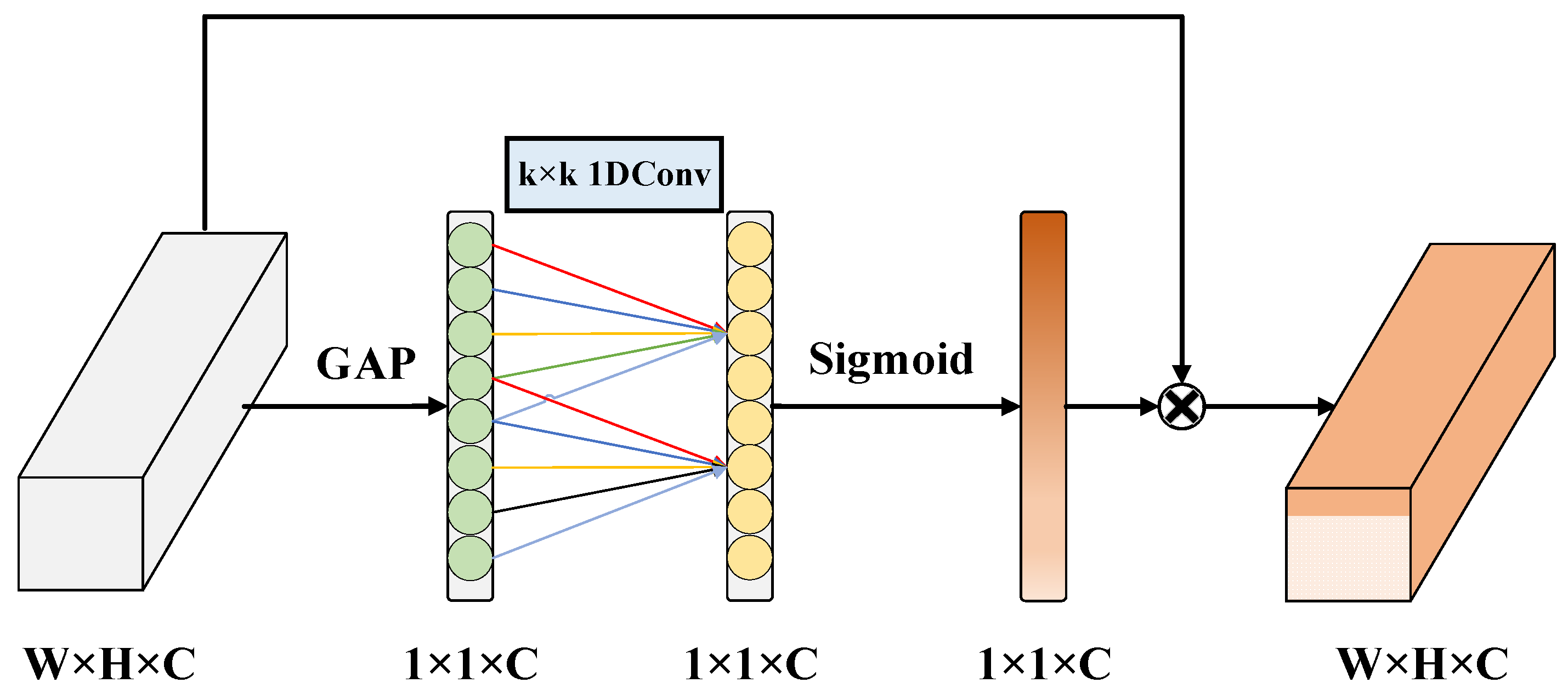
Pass the input feature map through global average pooling and transform it from a [h, w, c] matrix to a [1, 1, c] vector;

(2)

Calculate the size of adaptive one-dimensional convolution kernel size $k$ based on the number of channels in the feature map, $k=\left|{\displaystyle \frac{{\log }_2\left(c\right)}{\gamma }}+{\displaystyle \frac{b}{\gamma }}\right|$, and generally set $\gamma =2$, $b=1$;

(3)

Apply the kernel size to the one-dimensional convolution to obtain the weights for each channel of the feature map;

(4)

Multiply the normalized weights channel-wise with the original input feature map to generate the weighted feature map.

In terms of the overall network architecture design, all the convolutional layers in the network are uniformly structured as convolution + batch normalization + activation, which accelerates the convergence speed and enhances the generalization ability. Relative experiments demonstrate that the decomposition strategy of Inception V3 performs exceptionally well on feature maps of an intermediate size (m × m, where m ranges from 12 to 20) [41]. Therefore, the time-series input spans 20 points, and the input parameters are set to 12 according to the analysis in Section 3.2. Consequently, the input dimension is 20 × 12, ensuring the efficiency of the Inception V3 network. As the ECA attention mechanism does not alter the data dimensionality, the result of the channel concatenation of Inception V3 is directly fed into the ECA module. Then, it passes through fully connected layers and a SoftMax classifier to obtain the fault diagnosis result.

Table 1. The structure of the Inception V3 network.

Layer	Structure Parameters	Output Dimensions
Input	64 × 20 × 12	64 × 1 × 20 × 12
Conv	3 × 3 × 16	64 × 16 × 18 × 10
Max Pooling	2 × 2	64 × 16 × 9 × 5
Inception V3	1 × 1 × 32	64 × 128 × 9 × 5
	1 × 1 × 16/1 × 3 × 32/3 × 1 × 32
	1 × 1 × 16/(1 × 3 × 32/3 × 1 × 32)×2
	3 × 3/1 × 1 × 32
ECA	-	64 × 128 × 9 × 5
FC	-	64 × 7

shows the structure of the Inception V3 network adopted in this paper.

To illustrate the meaning of the structure parameters, take 1 × 1 × 32 as an example, which means the convolutional kernel size is 1 × 1, with 32 channels, and / represents the connection relationship. As for other settings, 64 stands for the batch size and 7 stands for the number of categories.

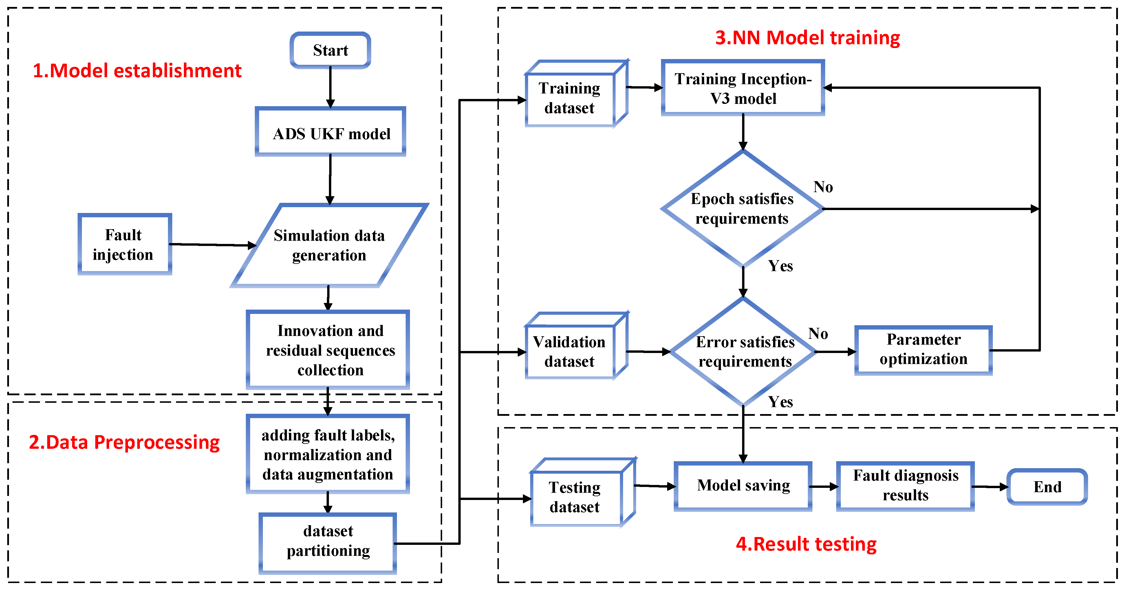
3.4. Overall Process of the Algorithm

The flowchart of the entire fault diagnosis algorithm is illustrated in Figure 6, depicting the main steps as follows:

(1)

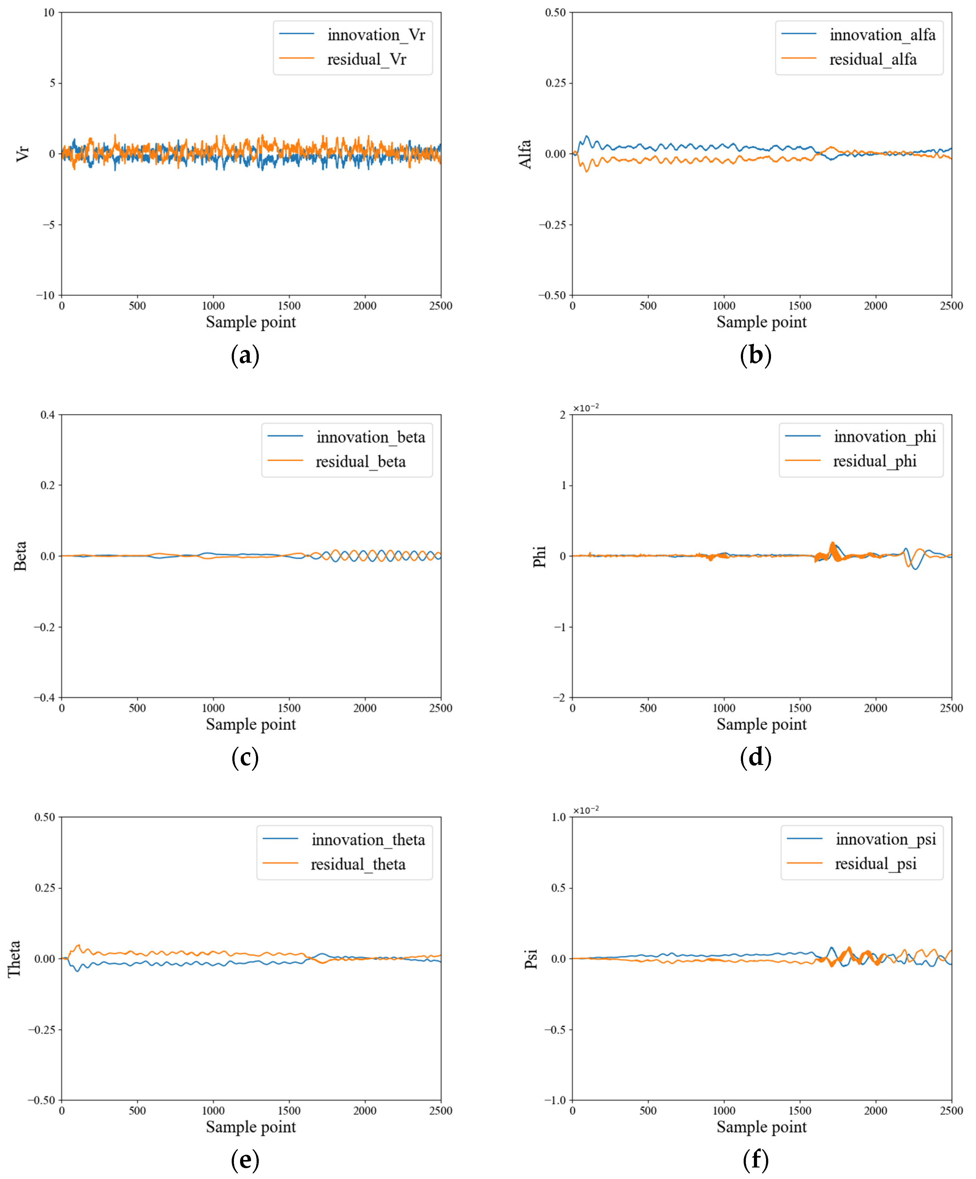
In the missile simulation model, the UKF model is established for the air data system, and abrupt and gradual faults are injected separately into the measurement sections of each sensor. Then, 12-dimensional innovation and residual sequences are collected under both normal and faulty conditions;

(2)

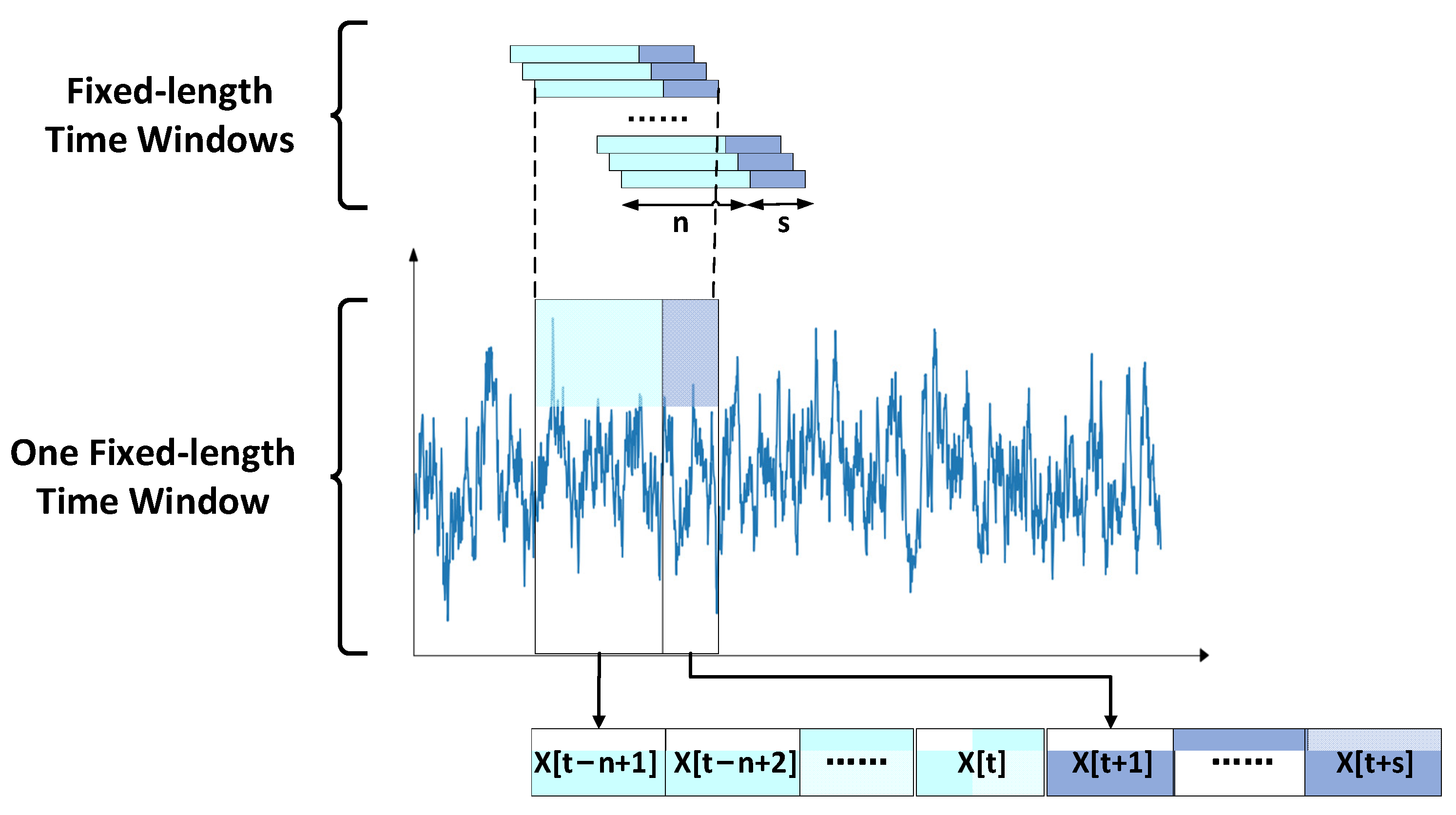
Preprocess the data, which includes adding fault labels; normalization; partitioning into training, validation, and testing datasets; and data augmentation through sliding windows;

(3)

Train the neural network model, where the loss function is chosen as the cross-entropy loss function, and the optimizer is Adam, by which the network parameters are updated during backpropagation;

(4)

Set the number of training epochs, and after reaching the desired error value and training epoch, test the model using the testing set and output the diagnostic results.

4. Experimental Validation

4.1. Dataset

To verify the applicability of the proposed algorithm, a missile system model is built on the Simulink simulation platform, with the BGM-109D cruise missile as the research object. As shown in Figure 7, the missile model consists of 6 modules, including the dynamics and kinematics of the missile, engine, rudder loop, control system, navigation system, and guidance system. The navigation system includes an INS/GPS integrated navigation system and air data system, with the UKF model embedded in the ADS section. Aiming at matching the actual flight scenarios of the missile, the environment model in the missile system adopts the 1976 International Standard Atmosphere model. The gravity model refers to the gravity calculation model in the World Geodetic System. The wind module utilizes the wind shear model and the Dryden wind turbulence model. The projectile parameters are set based on the Tomahawk cruise missile. To evaluate the algorithm’s performance under different trajectories, the target waypoints are randomly set within the range specified in

Table 2. Random range of the target waypoints.

	X (m)	Y (m)	Z (m)
Random Range	8000~12,000	−50~50	1000~2000

.

The air data system mainly includes sensors such as the airspeed indicator, angle of attack sensor, and sideslip angle sensor. These sensors may encounter faults caused by factors such as airspeed probe leakage, sensor component aging, and electromagnetic interference [45,46]. The fault manifestations on the sensor signals include a constant fault, abrupt fault, and gradual fault. Since diagnosing constant faults is relatively easy, this study mainly focuses on abrupt faults and gradual faults in the airspeed, angle of attack, and sideslip angle signals, and the fault manifestations are represented as the step fault and ramp fault, respectively. Denote the unit step function as $u\left(t-t_0\right)$ and the fault onset time as $t_0$, then the faults can be described as follows:

Step fault:

$$f\left(t\right)=Au\left(t-t_0\right)$$

(24)

where $A$ is the amplitude of the step fault.

Ramp fault:

$$f\left(t\right)=R\left(t-t_0\right)u\left(t-t_0\right)$$

(25)

where $R$ is the slope of the ramp fault.

In this fault setting scenario, without considering compound faults, there are 6 fault types as well as the normal state, which means a total of 7 scenarios. The flight time is set to 50 s, and the fault is randomly added in the range of 20~35 s. The simulation platform generates data points every 0.01 s, resulting in 5000 data points for each simulation. The fault types and settings are presented in

Table 3. Fault setting.

Fault Category	Fault Sensor	Label	Fault Severity	Training Samples	Testing Samples
Normal	-	0	-	500	100
Step Fault	Angle of attack	1	0.04~0.4 (°)	500	100
	Sideslip angle	2	0.02~0.2 (°)	500	100
	Airspeed	3	3~10 (m/s)	500	100
Ramp Fault	Angle of attack	4	0.001~0.01 (°/s)	500	100
	Sideslip angle	5	0.001~0.01 (°/s)	500	100
	Airspeed	6	0.05~0.5 (m/s2)	500	100

.

To enrich the dataset and enhance training effectiveness, sliding window is employed for data augmentation. The principle of sliding window is shown in Figure 8. Here, data are collected for 24 sample points (240 ms) following each fault occurrence, with a window length of 20 (200 ms) and a sliding step of 1. This increases the number of samples 5 times, obtaining 2500 samples for each fault scenario in the training dataset and 500 samples in the testing set.

4.2. Parameter Settings

For the UKF model, the formula for determining the first-order weight coefficient $W_i^m$ and the second-order weight coefficient $W_i^c$ in Equation (15) is:

$$\left\{\begin{array}{l}{W}_0^m={\displaystyle \frac{\lambda }{n+\lambda }}\\ W_0^c={\displaystyle \frac{\lambda }{n+\lambda }}+1-{{\alpha }_0}^2+{\beta }_0\\ W_i^m=W_i^c={\displaystyle \frac{1}{2\left(n+\lambda \right)}},i=1,2,\dots \dots ,2n\end{array}\right.$$

(26)

where $\lambda ={{\alpha }_0}^2\left(n+\kappa \right)-n$. The parameters ${\alpha }_0$ and $\kappa$ are ratio parameters that determine the range of the sigma point distribution around the mean. To ensure the distribution state of sigma points and the positive definiteness, $1\times {10}^{-4}\le {\alpha }_0\le 1$ and $\kappa \ge 0$. The parameter ${\beta }_0$ is used to introduce higher-order information of the state variable probability distribution. In the case of a Gaussian distribution, ${\beta }_0$ is set to 2. According to relative experience and testing, set $\kappa =0$, ${\alpha }_0=0.8$, ${\beta }_0=2$. The covariance matrix of process noise in Equation (15) $Q=diag\left(\left[1\times {10}^{-4},1\times {10}^{-4},1\times {10}^{-4},3\times {10}^{-8},3\times {10}^{-8},3\times {10}^{-8}\right]\right)$ and the covariance matrix of measurement noise in Equation (15) $R=diag\left(\left[1\times {10}^{-4},3\times {10}^{-6},3\times {10}^{-6},3\times {10}^{-8},3\times {10}^{-8},3\times {10}^{-8}\right]\right)$ $diag$ represent the diagonal matrix.

For the Inception network, the input dimension is 20 × 12, where 20 represents the number of sample points. Since the platform samples a point every 10 ms, it corresponds to a time window of 200 ms. The number 12 represents the data dimension, including 6 dimensions for innovations and those for residuals. The structural configuration can be seen in detail in Table 1. The model is built on the PyTorch framework, with a training/validation set ratio of 4:1. The loss function is cross-entropy, and the optimizer is Adam with a learning rate of 0.0005. The batch size and training epoch are 64 and 50, respectively.

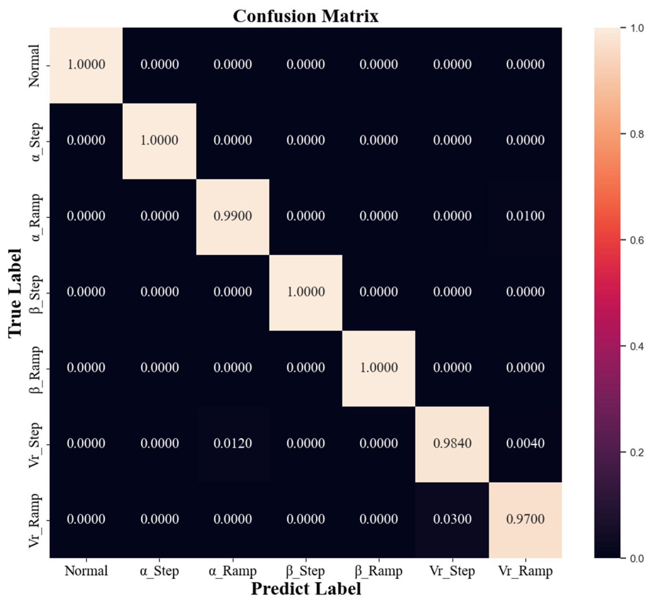
4.3. Results and Analysis

Under normal conditions, the innovation and residual sequences generated by the UKF model are shown in Figure 9. It can be observed that they fluctuate around zero in the absence of faults. However, when a fault occurs, it significantly disrupts this characteristic, which will be further illustrated by examples later on.

Model-based fault diagnosis methods generally involve constructing test statistics based on the information generated by the model and comparing them to a threshold to judge the occurrence of faults. However, on one hand, constructing evaluation metrics is often challenging. For example, the residual chi-squared test has low sensitivity to gradual faults, and many self-defined metrics are subjective, making it difficult to demonstrate their applicability to various types of faults. On the other hand, these methods often lack the ability to locate faulty sensors and identify the type of fault effectively after fault detection. Typically, setting thresholds for corresponding fault signals of sensors is subjective and difficult to account for variations caused by various uncertainties. Therefore, in addition to establishing the model, a data-driven approach is combined to complement the model-based fault diagnosis strategy. In this regard, the experimental results of the neural network component are presented.

Figure 10 illustrates the training process of the neural network model. After 50 epochs of training, the error gradually decreases and stabilizes at around 0.001. Testing was conducted on the testing dataset, and Figure 11 shows the confusion matrix. It can be observed that the Inception V3 network, based on UKF’s innovations and residuals as inputs, achieves ideal diagnostic results with diagonal elements in the confusion matrix close to 1. This indicates that it can effectively discriminate among various fault conditions, with only a small number of misclassifications.

We quantitatively analyzed the diagnostic results through three metrics: precision, recall, and F1 score. The closer these metrics are to 1, the better the diagnostic performance. According to the statistics, the accuracy of this method is 0.9920, the recall is 0.9920, and the F1 score is 0.9920. All metrics are above 99%, and the results can be obtained within 200 ms. It can be seen that the fault diagnosis strategy utilizing data-assisted models has achieved excellent results.

In the selection of fault characteristic data, to demonstrate the necessity of utilizing the UKF’s innovation and residual sequences, this study compares the results with those using raw data and innovation data only. The raw data refer to the filtered six-dimensional measurement signal sequences. Taking the gradual fault in the airspeed signal as an example, with a fault severity of 0.05 (m/s²) and fault injection time of 23.5 s (the 2350th data point), the filtered airspeed data, innovation sequence, and residual sequence are shown in Figure 12.

When the fault severity is small, the post-fault data do not exhibit significant changes compared to the original signal, and the data have some inherent fluctuations. It is difficult to judge whether the observed variations are normal or indicative of a fault compared to the pre-fault condition, and fault diagnosis based solely on the fault signal becomes challenging. Although innovations can also reveal some changes, due to the iterative nature of the filtering process, the subsequent innovations continuously track the fault and exhibit minor fluctuations when dealing with small fault severities. This contradicts the essence of gradual deterioration caused by a gradual fault over time. Therefore, the addition of residuals assists in fault diagnosis. It can effectively reflect the fault condition as time progresses and the fault severity increases.

The t-distributed stochastic neighbor embedding (t-SNE) algorithm is employed to visualize the classification effectiveness of features, which is shown in Figure 13. It can be observed that the result based on the innovation and residual sequences of the UKF, after feature extraction via the Inception V3 network, exhibits a significant improvement in fault discrimination, and only a small number of samples are misclassified. In contrast, the other two show a substantial overlap in the feature regions, indicating the difficulty in distinguishing fault conditions. The fault diagnosis results for the three types of data under the same model are shown in

Table 4. Diagnostic results for the innovation and residual sequences, raw signal data, and innovation sequences.

	Innovation and Residual	Innovation	Filtered Data
Precision	0.9920	0.8057	0.8897
Recall	0.9920	0.8057	0.8897
F1 Score	0.9920	0.7830	0.8898

.

From the results, it can be seen that, in scenarios with low fault severity and varied experimental settings, relying solely on the fault signal for diagnosis does not yield satisfactory results. As mainstream information used for fault diagnosis, innovations exhibit obvious limitations when it comes to diagnosing small faults and gradual faults. It becomes difficult to distinguish them from normal conditions, and the diagnostic performance is even poorer at times. The combination of innovations and residuals overcomes the aforementioned problems and achieves better diagnostic results.

In order to better simulate actual conditions, a certain level of Gaussian noise was added to the collected airspeed, angle of attack, and sideslip angle signals. This was conducted to test the ability of the proposed method to accurately identify faults when they are submerged in noise and to verify its robustness against significant noise interference. According to relevant research, the signal-to-noise ratio (SNR) is typically around tens of decibels (dB), where a lower signal-to-noise ratio indicates a higher level of noise. As an example, an SNR of 40 dB was chosen to conduct further experiments.

Furthermore, to validate the superiority of the neural network used in this paper, a comparison was made with other commonly used networks, including the convolutional neural network (CNN), fully convolutional network (FCN) [47], and temporal convolutional network (TCN) [48]. To ensure fairness in the comparison, the inputs for all neural networks are based on the innovations and residuals generated by the same unscented Kalman filter, and the same test dataset was employed to conduct tests and obtain fault diagnosis results, including accuracy, recall, F1 score, and the number of model parameters.

In the process of this new experiment, k-fold cross-validation was employed to reduce overfitting and improve generalization ability. Unlike the conventional approach of dividing the dataset into training and testing sets with a certain ratio, k-fold cross-validation divides the entire dataset into k mutually exclusive subsets. In each iteration, k-−1 subsets are used for training, while the remaining subset is used for testing. This process is repeated until each subset has been used as the test set. This generates k evaluation metrics, and the final result is obtained by calculating the mean and variance of these metrics.

k is set to 5 in this experiment, and the performance metrics of different networks are shown in

Table 5. Diagnostic results of different networks.

	Inception V3 + ECA	Inception V3	CNN	FCN	TCN
Precision	0.9725	0.9668	0.9299	0.9064	0.9447
Recall	0.9728	0.9668	0.9304	0.9062	0.9443
F1 Score	0.9726	0.9669	0.9307	0.9069	0.9447
Model Parameters	58,284	58,279	97,670	94,023	117,319

, where the results presented are the average values obtained after five iterations. Figure 14 shows the error bar plot according to different means and errors.

From the experimental results, it can be observed that, by extracting innovation and residual sequences of the UKF, the fault features are distinctly represented, and all the neural networks achieve relatively good results. Among them, the Inception V3 network, with its ability to extract features at multiple scales, demonstrated a superior performance in handling multiple fault types, even in situations with relatively high levels of noise interference. Other neural networks, due to reasons such as slow convergence speed and an inability to accurately extract fault features, exhibit a relatively poorer performance in such situations. Additionally, Inception V3 maintains network sparsity while ensuring a good performance, as it has significantly fewer parameters compared to other networks. This achieves a balance between network performance and computational resources. Furthermore, the inclusion of the ECA attention mechanism strengthens the influence of key features, leading to further improvements in performance with a minimal increase in the number of parameters. The above experiments demonstrate the effectiveness and advantages of the proposed approach based on the UKF and Inception V3 model for fault diagnosis in the missile air data system.

5. Conclusions

This paper proposes a fault diagnosis method for a missile air data system based on the UKF and the Inception V3 network, which extracts innovation and residual sequences from the UKF model of the ADS as the input of the Inception V3 network, and comparative experiments demonstrate the advantages of the proposed method. Based on the analysis and experiments, the following conclusions can be drawn:

(1)

Based on the working mechanism of the ADS and the missile kinematic equations, the UKF model of the ADS is established to provide a more accurate description of the system. This avoids the problems of distinguishing faults from changes in flight states that are commonly encountered in purely data-driven methods.

(2)

Instead of using hypothesis testing methods, such as chi-squared tests in the diagnostic process, the proposed method extracts innovation and residual sequences from the UKF model to amplify fault features and employs them as inputs to the neural network, which better reflects fault conditions compared to traditional methods based on filtered data or innovation data.

(3)

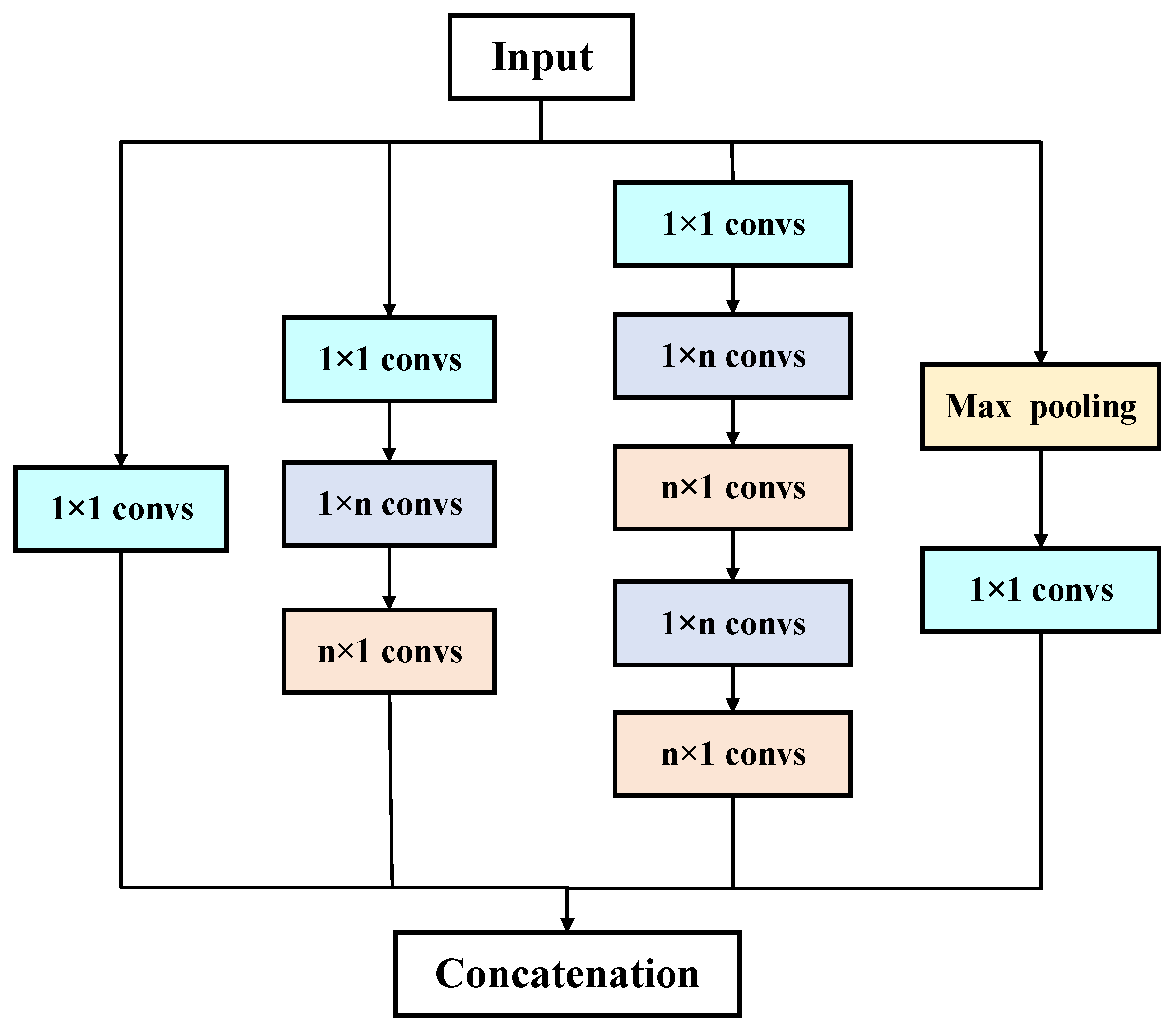
The Inception V3 network is designed, which extracts features in parallel at multiple scales while ensuring high computational efficiency by leveraging the principles of sparse matrices. Additionally, the network incorporates the lightweight ECA attention mechanism to further enhance the diagnostic performance.

The proposed method, through the integration of model and data, effectively addresses the limitations of model-based approaches relying on hypothesis testing or subjective settings, as well as the performance degradation of data-driven methods under variable environmental conditions, which provides a new train of thought for the fault diagnosis of missile air data systems.

This study still has some limitations, which are reflected in the relatively ideal setting of fault modes, and it may deviate from actual conditions and fail to consider all possible scenarios. Additionally, there is room for improvement in the establishment of the UKF model and Inception V3 network. In further research, we will delve into more complex scenarios and faults for missile air data systems. This may involve considering the mechanism and modeling of the pitot tube, angle of attack, and sideslip angle sensors, for example, as well as constructing a computational model for the air data computer. Meanwhile, this study focused on cruise missiles as the experimental subject, and future considerations include validating the proposed methods for other types of missiles. Moreover, by incorporating methods such as adaptive strategies and optimization algorithms, we hope to further optimize the UKF model and Inception V3 network to enhance accuracy and reliability.

References

- Nebula, F.; Palumbo, R.; Morani, G. Virtual air data: A fault-tolerant approach against ADS failures. In Proceedings of the AIAA Infotech@ Aerospace (I@ A) Conference, Boston, MA, USA, 19–22 August 2013; p. 4568. [Google Scholar]
- Wan, Y.; Keviczky, T.; Verhaegen, M. Robust air data sensor fault diagnosis with enhanced fault sensitivity using moving horizon estimation. In Proceedings of the 2016 American control conference (ACC), Boston, MA, USA, 6–8 July 2016; pp. 5969–5975. [Google Scholar]
- Fravolini, M.L.; Del Core, G.; Papa, U.; Valigi, P.; Napolitano, M.R. Data-driven schemes for robust fault detection of air data system sensors. IEEE Trans. Control. Syst. Technol. 2017, 27, 234–248. [Google Scholar] [CrossRef]
- Houck, D.; Atlas, L. Air data sensor failure detection. In Proceedings of the 17th DASC. AIAA/IEEE/SAE. Digital Avionics Systems Conference, Bellevue, WA, USA, 31 October–7 November 1998; Volume 1, p. D17-1. [Google Scholar]
- Li, D.; Wang, Y.; Wang, J.; Wang, C.; Duan, Y. Recent advances in sensor fault diagnosis: A review. Sens. Actuators A Phys. 2020, 309, 111990. [Google Scholar] [CrossRef]
- Nandi, S.; Toliyat, H.A.; Li, X. Condition monitoring and fault diagnosis of electrical motors—A review. IEEE Trans. Energy Convers. 2005, 20, 719–729. [Google Scholar] [CrossRef]
- Zhu, Z.Q.; Liang, D.; Liu, K. Online parameter estimation for permanent magnet synchronous machines: An overview. IEEE Access 2021, 9, 59059–59084. [Google Scholar] [CrossRef]
- Wang, Z.; Liu, C. Wind turbine condition monitoring based on a novel multivariate state estimation technique. Measurement 2021, 168, 108388. [Google Scholar] [CrossRef]
- Song, Y.; Zhong, M.; Xue, T.; Ding, S.X.; Li, W. Parity space-based fault isolation using minimum error minimax probability machine. Control. Eng. Pract. 2020, 95, 104242. [Google Scholar] [CrossRef]
- Guo, D.; Zhong, M.; Zhou, D. Multisensor data-fusion-based approach to airspeed measurement fault detection for unmanned aerial vehicles. IEEE Trans. Instrum. Meas. 2017, 67, 317–327. [Google Scholar] [CrossRef]
- Xiong, H.; Bian, R.; Li, Y.; Du, Z.; Mai, Z. Fault-tolerant GNSS/SINS/DVL/CNS integrated navigation and positioning mechanism based on adaptive information sharing factors. IEEE Syst. J. 2020, 14, 3744–3754. [Google Scholar] [CrossRef]
- Yun, S.H.; Kang, C.W.; Park, C.G. Reducing the computation time in the state chi-square test for IMU fault detection. In Proceedings of the 2014 14th International Conference on Control, Automation and Systems (ICCAS 2014), Gyeonggi-do, Republic of Korea, 22–25 October 2014; pp. 879–883. [Google Scholar]
- Wang, R.; Xiong, Z.; Liu, J.; Xu, J.; Shi, L. Chi-square and SPRT combined fault detection for multisensor navigation. IEEE Trans. Aerosp. Electron. Syst. 2016, 52, 1352–1365. [Google Scholar] [CrossRef]
- Wan, Y.; Puig, V.; Ocampo-Martinez, C.; Wang, Y.; Harinath, E.; Braatz, R.D. Fault detection for uncertain LPV systems using probabilistic set-membership parity relation. J. Process Control. 2020, 87, 27–36. [Google Scholar] [CrossRef]
- Blesa, J.; Puig, V.; Saludes, J. Robust identification and fault diagnosis based on uncertain multiple input–multiple output linear parameter varying parity equations and zonotopes. J. Process Control. 2012, 22, 1890–1912. [Google Scholar] [CrossRef]
- Zhong, M.; Song, Y.; Ding, S.X. Parity space-based fault detection for linear discrete time-varying systems with unknown input. Automatica 2015, 59, 120–126. [Google Scholar] [CrossRef]
- Lu, P.; Van Eykeren, L.; Van Kampen, E.; De Visser, C.C.; Chu, Q.P. Adaptive three-step Kalman filter for air data sensor fault detection and diagnosis. J. Guid. Control. Dyn. 2016, 39, 590–604. [Google Scholar] [CrossRef]
- Lu, P.; Van Kampen, E.J.; De Visser, C.; Chu, Q. Air data sensor fault detection and diagnosis in the presence of atmospheric turbulence: Theory and experimental validation with real flight data. IEEE Trans. Control. Syst. Technol. 2020, 29, 2255–2263. [Google Scholar] [CrossRef]
- Freeman, P.; Seiler, P.; Balas, G.J. Air data system fault modeling and detection. Control. Eng. Pract. 2013, 21, 1290–1301. [Google Scholar] [CrossRef]
- Fravolini, M.L.; Napolitano, M.R.; Del Core, G.; Papa, U. Experimental interval models for the robust fault detection of aircraft air data sensors. Control. Eng. Pract. 2018, 78, 196–212. [Google Scholar] [CrossRef]
- Prabhu, S.; Anitha, G. An innovative analytic redundancy approach to air data sensor fault detection. Aeronaut. J. 2020, 124, 346–367. [Google Scholar] [CrossRef]
- Van Eykeren, L.; Chu, Q. Air Data Sensor Fault Detection using Kinematic Relations. In Advances in Aerospace Guidance, Navigation and Control: Selected Papers of the Second CEAS Specialist Conference on Guidance, Navigation and Control; Springer: Berlin/Heidelberg, Germany, 2013; pp. 183–197. [Google Scholar]
- Kalaiarasi, G.; Maheswari, S. Deep proximal support vector machine classifiers for hyperspectral images classification. Neural Comput. Appl. 2021, 33, 13391–13415. [Google Scholar] [CrossRef]
- Yi, H.; Song, X.-F.; Jiang, B.; Liu, Y.-F.; Zhou, Z.-H. Flexible support vector regression and its application to fault detection. Acta Autom. Sin. 2013, 39, 272–284. [Google Scholar] [CrossRef]
- Sun, Y.; Li, S. Bearing fault diagnosis based on optimal convolution neural network. Measurement 2022, 190, 110702. [Google Scholar] [CrossRef]
- Chung, S.; Abbott, L.F. Neural population geometry: An approach for understanding biological and artificial neural networks. Curr. Opin. Neurobiol. 2021, 70, 137–144. [Google Scholar] [CrossRef] [PubMed]
- Chen, M.; Tao, G.; Jiang, B. Dynamic surface control using neural networks for a class of uncertain nonlinear systems with input saturation. IEEE Trans. Neural Netw. Learn. Syst. 2014, 26, 2086–2097. [Google Scholar] [CrossRef]
- Xu, H.; Lian, B. Fault detection for multi-source integrated navigation system using fully convolutional neural network. IET Radar Sonar Navig. 2018, 12, 774–782. [Google Scholar] [CrossRef]
- Xia, S.; Zhou, X.; Shi, H.; Li, S.; Xu, C. A fault diagnosis method based on attention mechanism with application in Qianlong-2 autonomous underwater vehicle. Ocean. Eng. 2021, 233, 109049. [Google Scholar] [CrossRef]
- Wen, X.; Ji, L.; Zhang, X.; Zhao, J. Fault Detection and Diagnosis in the INS/GPS Navigation System; World Automation Congress (WAC): Waikoloa, HI, USA, 2014; pp. 27–32. [Google Scholar]
- Guan, Y.; Meng, Z.; Sun, D.; Liu, J.; Fan, F. 2MNet: Multi-sensor and multi-scale model toward accurate fault diagnosis of rolling bearing. Reliab. Eng. Syst. Saf. 2021, 216, 108017. [Google Scholar] [CrossRef]
- Zhang, Q.; Wang, X.; Xiao, X.; Pei, C. Design of a fault detection and diagnose system for intelligent unmanned aerial vehicle navigation system. Proc. Inst. Mech. Eng. Part C J. Mech. Eng. Sci. 2019, 233, 2170–2176. [Google Scholar] [CrossRef]
- Min, H.; Fang, Y.; Wu, X.; Lei, X.; Chen, S.; Teixeira, R.; Zhu, B.; Zhao, X.; Xu, Z. A fault diagnosis framework for autonomous vehicles with sensor self-diagnosis. Expert Syst. Appl. 2023, 224, 120002. [Google Scholar] [CrossRef]
- Alqurashi, M.; Wang, J. Performance analysis of fault detection and identification for multiple faults in GNSS and GNSS/INS integration. J. Appl. Geod. 2015, 9, 35–48. [Google Scholar] [CrossRef]
- Zuo, J.; Ding, J.; Feng, F. Latent Leakage Fault Identification and Diagnosis Based on Multi-Source Information Fusion Method for Key Pneumatic Units in Chinese Standard Electric Multiple Units (EMU) Braking System. Appl. Sci. 2019, 9, 300. [Google Scholar] [CrossRef]
- Zhu, Y.; Cheng, X.; Wang, L. A novel fault detection method for an integrated navigation system using Gaussian process regression. J. Navig. 2016, 69, 905–919. [Google Scholar] [CrossRef]
- Pirmoradi, F.N.; Sassani, F.; De Silva, C.W. Fault detection and diagnosis in a spacecraft attitude determination system. Acta Astronautica 2009, 65, 710–729. [Google Scholar] [CrossRef]
- Zhao, Y.; Chen, Y.; Chen, L.; Deng, X.; Jiang, N.; Hou, L. Intelligent Fault Diagnosis Method for AUV Integrated Navigation System. In Proceedings of the 2021 IEEE International Conference on Unmanned Systems (ICUS), Beijing, China, 15–17 October 2021; pp. 896–901. [Google Scholar]
- Sadhukhan, C.; Mitra, S.K.; Naskar, M.K.; Sharifpur, M. Fault diagnosis of a nonlinear hybrid system using adaptive unscented Kalman filter bank. Eng. Comput. 2022, 38, 2717–2728. [Google Scholar] [CrossRef]
- Zhang, C.; Guo, C.; Zhang, D. Data Fusion Based on Adaptive Interacting Multiple Model for GPS/INS Integrated Navigation System. Appl. Sci. 2018, 8, 1682. [Google Scholar] [CrossRef]
- Stefenon, S.F.; Yow, K.C.; Nied, A.; Meyer, L.H. Classification of distribution power grid structures using inception v3 deep neural network. Electr. Eng. 2022, 104, 4557–4569. [Google Scholar] [CrossRef]
- Lin, P.; Qian, Z.; Lu, X.; Lin, Y.; Lai, Y.; Cheng, S.; Chen, Z.; Wu, L. Compound fault diagnosis model for photovoltaic array using multi-scale SE-ResNet. Sustain. Energy Technol. Assess. 2022, 50, 101785. [Google Scholar] [CrossRef]
- Zhu, Y.; Pei, Y.; Wang, A.; Xie, B.; Qian, Z. A partial domain adaptation scheme based on weighted adversarial nets with improved CBAM for fault diagnosis of wind turbine gearbox. Eng. Appl. Artif. Intell. 2023, 125, 106674. [Google Scholar] [CrossRef]
- Shi, Y.; Wang, Z.; Du, X.; Ling, G.; Jia, W.; Lu, Y. Research on the membrane fouling diagnosis of MBR membrane module based on ECA-CNN. J. Environ. Chem. Eng. 2022, 10, 107649. [Google Scholar] [CrossRef]
- Sun, K.; Gebre-Egziabher, D. A fault detection and isolation design for a dual pitot tube air data system. In Proceedings of the 2020 IEEE/ION Position, Location and Navigation Symposium (PLANS), Portland, OR, USA, 20–23 April 2020; pp. 62–72. [Google Scholar]
- Ossmann, D. Enhanced detection and isolation of angle of attack sensor faults. In Proceedings of the AIAA Guidance, Navigation, and Control Conference, San Diego, CA, USA, 4–8 January 2016; p. 1135. [Google Scholar]
- Karim, F.; Majumdar, S.; Darabi, H.; Chen, S. LSTM fully convolutional networks for time series classification. IEEE Access 2017, 6, 1662–1669. [Google Scholar] [CrossRef]
- Zhang, H.; Ge, B.; Han, B. Real-Time Motor Fault Diagnosis Based on TCN and Attention. Machines 2022, 10, 249. [Google Scholar] [CrossRef]