Study on the Flow Velocity of Safe and Energy-Saving Transportation of Light-Particle Slurry

Abstract

In order to determine the recommended flow velocity for the safe and energy-saving transport of ice-slurry-type light particle slurries, it is necessary to study the flow characteristics of light particle slurries, especially the critical flow velocity. Therefore, in this paper, a numerical simulation method based on the mixed turbulence model with the RANS (Reynolds averaged Navier Stokes) equation is used, and a new concentration distribution method is proposed for the first time to derive the critical flow velocity, as follows: the flow velocity of the light particle slurry when the ratio of the solid volume fraction vf at the position of 0.08D above the bottom of the pipeline to that at the center of the pipeline, vf/vf(y) = 0.75, is taken as the critical flow velocity. The flow changes in the slurry (polyethylene particles with a density of 922 kg/m³ and water) under 0.1–1.0 m/s (at intervals of 0.1 m/s) were investigated experimentally, and the pressure drop data obtained from the experiments were used to determine the recommended flow rate for safe and energy-saving transportation of the light particle slurry. The pipe diameter used for the experiments and simulations was 28 mm, and the solid-phase particle sizes were 0.3 mm, 0.4 mm, and 0.5 mm, with solid-phase contents of 5 vol%, 10 vol%, 15 vol%, and 20 vol%. In addition, the experimental and numerical simulation results show that an increase in solid-phase content and particle size leads to an increase in critical flow velocity.

1. Introduction

Ice slurry is a solid–liquid mixed two-phase refrigerant consisting of ice crystal particles, water, and a freezing point modifier, where the average characteristic diameter of the ice crystal particles does not exceed 1 mm [1]. Due to its excellent heat transfer characteristics and flow properties, ice slurry is considered a promising and premium fluid [2]. Ice slurry, as a cold storage medium, is one of the most effective means to realize the “peak shifting and valley filling” of the power grid [3], and it has been widely used in the fields of cold storage in buildings, food cooling, mine cooling, and medical protection [4]. In addition, polymer-oil-driving technology and hydraulic transportation of gelled crude oil in oil fields [5,6], polymer particle–water solid–liquid two-phase flow of polypropylene, polyethylene, and other polymers in annular tube reactors [7], solid–liquid two-phase flow of hollow glass beads–water in the preparation of lightweight cement composites for water purification and lightweight cement composites [8,9], and so on, are all flow problems that are part of the light particles two-phase flow model. Therefore, it is important to find out the optimal flow rate for the safe and energy-efficient transportation of light particle slurries. Therefore, the safe transportation of ice slurries in pipelines plays a crucial role for their application in practice.

Critical flow velocity is an important parameter for slurry pipeline transportation, which refers to the minimum safe flow rate required to ensure the flow of slurry. An unreasonable working flow velocity not only leads to solid-phase particles becoming gathered in the pipeline to cause pipeline wear and pipeline clogging [10], but also leads to an increase in conveying resistance and improves the energy consumption of the system; therefore, a reasonable determination of the size of the critical flow velocity is an effective means to ensure the safe and economic transportation of slurry. At present, the definition of critical flow velocity for slurry is not the same as that of other scholars. Harbottle [11] and Januário [12] used the “minimum conveying flow velocity” and “critical deposition flow velocity” as the definition of critical flow velocity, respectively. Wang [13] believed that the critical flow velocity is the flow velocity that causes the phenomenon of pipeline erosion and corrosion in the pipeline transportation of solid–liquid two-phase flow. The flow states of ice slurry in the pipe are generally categorized into three, as follows: stationary bed, moving bed, and suspended bed [14]. In the suspended bed, it is subdivided into a non-homogeneous bed and a homogeneous bed, according to the distribution of the ice crystal particles. In order to avoid ice jamming phenomenon and enable the ice slurry to be transported safely and stably, the critical flow velocity of the ice slurry is considered to be the velocity when the flow pattern is exactly changed from a moving bed to a non-homogenized suspended bed [15]. Currently, various scholars have proposed many critical flow rate calculation methods, as well as empirical or semi-empirical formulas [16,17,18,19], which are of some guiding significance for slurry transportation. However, due to the limitation of experimental content and experimental methods, it cannot comprehensively consider all of the factors in pipeline hydraulic conveying, and many formulas have their limitations. Rawat [20] analyzed the influence of ice slurry concentration distribution on the flow by numerical simulation and found that the flow tends to show more homogeneous distribution flow with the increase in inlet flow velocity, the increase in ice content rate, and the decrease in particle size. This method can effectively determine the ice slurry flow pattern based on the degree of particle stratification, thus determining the critical flow velocity; however, it is easy to produce errors through the iterative processing of simulation. Tian [21] regarded the ice crystal particles as a simple cubic arrangement and determined the critical flow velocity by using the maximum filling rate of the particles at the top of the pipeline (52%) as a discriminant of the ice slurry flow pattern. Although the method can obtain a safer critical flow velocity, it is not possible to determine the critical flow rate due to the fact that the complexity of the solid–liquid two-phase flow in the transport process and the size of the critical flow velocity may be overestimated. Wu [22] et al. established a multiphase flow model of Euler fluid in a pipe using Fluent software, studied the effects of initial IPF, particle size, and radius of curvature on the critical flow velocity of the pipe, and found that the critical flow velocity increased continuously with the increase in the initial ice content rate and the particle size, while the critical flow velocity decreased continuously with the increase in the radius of curvature of the bent pipe decreasing. Rayhan [23] investigated the pressure drop and non-Newtonian behavior of ice slurries in horizontal pipelines with a reduced freezing point of methanol at different methanol concentrations (8–25%) and ice mass fractions (0–29%). It was found that the pressure drops of the ice slurry in the horizontal pipe increased with increasing flow velocity and ice mass fraction. The flow velocity and ice mass fraction showed a dominant effect on the Reynolds number. Newtonian fluid behavior was observed at ice mass fractions of 3% to 5%, while pseudoplastic behavior was observed at ice mass fractions of 9% to 26%. In addition, the critical velocity is closely related to the flow pattern, and the flow pattern of two-phase flow is also one of the focuses of research [24].

In view of this, this paper presents a numerical simulation method for determining the critical flow rate of a light particle slurry in horizontal circular pipe transport. We consider that the melting and agglomeration of ice crystals will affect the density and particle size of the slurry, and both the density and particle size will have an effect on the critical flow velocity. Therefore, in this paper, polyethylene particles with a density of about 922 kg/m³ are selected to replace the ice crystal particles for the experimental and numerical simulation of slurry flow. The critical flow velocity under different working conditions is obtained through experimental observation, and the accuracy of the numerical simulation method is verified. Finally, the effects of solid-phase content and particle size on the critical flow rate are analyzed, and the flow pattern is compared with the pressure drop data. It was found that, when the slurry was in a moving bed or a stationary bed and transformed into a non-homogeneous suspended bed, there was an increase in the flow rate with a decrease in the pressure drop, which was favorable to the safe and energy-saving transportation of the slurry. When the flow rate is greater than the critical flow rate, the slurry is in a homogeneous suspended bed, where the flow rate increases the pressure drop of the slurry, which then increases rapidly, which is not conducive to the energy-saving transportation of the slurry. It was finally determined that the recommended flow rate for safe energy-saving transportation of slurry in the pipeline is the critical flow rate, and it was found that, when the solid-phase content is constant, the smaller the particle size is, and the more favorable it is for safe energy-saving transportation of slurry. This conclusion can achieve slurry transport in the horizontal circular pipe without clogging and can avoid increasing the transportation cost of the slurry, which is of great significance for the safe and energy-saving transportation of light-grained slurry in horizontal circular pipes in engineering applications.

2. Experimental Method

2.1. Experimental Setup

The design of the experimental scheme is shown in Figure 1, and the experimental system consists of the following three parts: the refrigerant-carrying circulation system, the pressure drop test system, and the data acquisition system. Figure 2 shows a physical diagram of the experimental setup, in which the low temperature and constant temperature circulator provides a constant temperature for the ice slurry flow during the experiment. The pressure drop test system consists of a storage tank, a stirring motor, a circulation pump, an electromagnetic flow meter, a test tube section, a thermocouple, a differential pressure transmitter, and a pressure sensor. The ice slurry storage device is a stainless-steel tank with the following dimensions: an outer diameter of 80 cm, an inner diameter of 60 cm, and a height of 100 cm, with a filling port at the top to facilitate the addition of experimental materials. The specific parameters of the experimental equipment are shown in

Table 1. Specific parameters of the experimental equipment.

Equipment Name	Product Model	Specifications	Company
Stirring motor	BLD09-11-0.75	Speed: 150 r/min	Yixing Yuanjia Environmental Protection Equipment (Yixing, China)
Circulating pump	25GW8-22	Speed: 2900 r/min; Rate of flow: 8 m3/h; Lift: 22 m	Kaiping Danai Pump Manufacturing Co., Ltd. (Kaiping, China)
Electromagnetic flowmeter	TBD-20Y-F4-1-A-1-16-A	Range: 0–6 m3/h; Precision: ±0.5%	Dalian Measuring Machinery Co. (Dalian, China)
Differential pressure transmitter	3051CD2A22B1AB415M5HR5	Range: 0–30 kPa; Precision: ±0.06%	Emerson Electric Company (St. Louis, MO, USA)
Thermocouple	K-type	Precision: ±0.1 °C	Shanghai No. 3 Electric Instrument Factory (Shanghai, China)
Pressure-drop sensor	PCM300	Range: 0–100 kPa; Precision: ±0.5%	Suzhou Xuan sheng Instrument Technology Co., Ltd. (Suzhou, China)
Low temperature and constant temperature circulator	DL-3030	The temperature range is −30~50 °C and the cooling capacity is 1000~3000 W.	Shanghai Qixun Instrument Co., Ltd. (Shanghai, China)

. The data acquisition system adopts the intelligent equipment monitoring module produced by Changsha Zhong Deng, which is able to display, record, and save all of the measured parameters in the experimental process in real time, and the recording time interval is 10 s. The test tube section is a highly transparent Plexiglas round tube, which is used to visualize the experimental observation of the slurry’s flow pattern, as well as the measurement of the flow resistance. The temperature and differential pressure measurement positions are shown in Figure 3.

2.2. Experimental Materials

The solid-phase particle size will have an effect on the flow pattern and critical flow velocity of the slurry. While ice slurry has a series of kinetic behaviors, such as ice particle agglomeration, melting, and fragmentation, during storage and flow [25,26,27], it is difficult to control the size of ice particles. In order to eliminate the effect of the change in the particle size of the ice crystal particles, polyethylene particles with a similar density to the ice crystal particles (density of 922 kg/m³) were used for the experiments. Three particle size ranges of polyethylene particles were screened through a mesh sieve. Fifty samples of each particle size were taken randomly, the maximum and minimum particle sizes of each sample were measured with vernier calipers (accuracy ±0.03 mm), and the average value was taken as the actual size of the experimental solid-phase particles, resulting in three types of polyethylene particles with average particle sizes of 0.3 mm, 0.4 mm, and 0.5 mm. The Figure 4 shows the microstructure of the three sizes of polyethylene particles under the microscope. The liquid phase medium was made of homemade pure water from the laboratory. For the solid–liquid two-phase flow studied in this paper, the densities of the solid and liquid phases were kept as constants. The solid-phase particle density was 922 kg/m³ and the liquid phase density was 999.969 kg/m³.

2.3. Experimental Steps and Working Conditions

Firstly, inject 135 L of pure water into the storage tank (the liquid phase water level is about 10 cm above the stirring blade). Turn on the stirring motor and adjust the speed to 150 r/min. Turn on the circulation pump and exhaust the conduit of the differential pressure transmitter until the reading of the differential pressure gauge stabilizes. Open the low-temperature thermostatic water tank and control the experimental temperature at about 3 °C. Use the electronic weighing scale (model ZCS, accuracy ±1 g) to weigh the polyethylene particles with a solid-phase content of 5 vol%, add them to the storage tank, and stir for 2–3 min to form a solid–liquid mixture. Then, adjust the flow valve according to the flow rate of each flow velocity and record the value of the pressure drop and the flow pattern when it is stabilized. Then, add the polyethylene particles with a solid-phase content of 10%, 15%, and 20% in turn to the storage tank and record the resulting pressure drop in turn. Then, add 10%, 15%, and 20% solid phase polyethylene particles to the storage tank and record the pressure drop and flow pattern in turn. After the above work is completed, turn off all experimental equipment and discharge the slurry in the tank from the drain below the storage tank. Then, add pure water to the tank, turn on the equipment, and clean the piping. Finally, discharge the water from the storage tank and complete all experiments. Sequentially replace the different-sized particles to continue the experiment until all conditions of the experiment are completed. The specific experimental conditions are shown in

Table 2. Experimental conditions and relative error.

Name	Working Condition Parameters	Relative Error
Flow velocity: v/m·s−1	0.1~1	0.51%
Pipe diameter: D/mm	17, 24, 28	0.0001%
Solid particle size: d/mm	0.3, 0.4, 0.5	/
Solid content (IPF): Cv/vol%	0, 5, 10, 15, 20	0.001%
ΔP/Pa	/	0.06%
T/°C	/	0.1%

. In addition, we show, in

Table 3. Constants that appear in equations and coefficients.

Notation	Hidden Meaning	Numerical Value	Unit
ds	Particle size	0.3, 0.4, 0.5	mm
g	Gravitational acceleration	9.81	m/s2
$K_{Sl}$	Momentum transfer coefficient between two phases	-	-
ρ	Density	Solid phase: 922, Liquid phase: 1000	kg/m3
α	Volume fraction	5, 10, 15, 20	%
Cμ	Empirical constant	0.09	-
${\sigma }_k$	The inverse effective Prandtl coefficient of k	1	-
${\sigma }_{\epsilon }$	The inverse effective Prandtl coefficient of ε	1.3	-
$C_{1\epsilon }$$,C_{2\epsilon }$	The lift coefficient of ε	1.44, 1.92
M	Momentum exchange between two phases	-	kg·m−2·s−2
μ	Shear viscosity	-	kg·m−1·s−1
λ	Body viscosity coefficient	-	kg·m−1·s−1
${\sigma }_D$	Prandtl factor	-	-
Cl	Coefficient of lift	-	-
$e_{ss}$	Particle collision recovery coefficient		-
${\mu }_{s,skin}$	Kinetic viscosity	-	kg·m−1·s−1
${\mu }_{s,col}$	Crash viscosity	-	kg·m−1·s−1
${\mu }_{s,fr}$	Friction viscosity	-	kg·m−1·s−1
${\mu }_{t,m}$	Turbulent viscosity	-	kg·m−1·s−1

, the symbols covered in this paper, as well as their meanings and units. In addition, the specific experimental method is shown in the form of a flowchart in Figure 5.

2.4. Error Analysis

The direct measurement errors during the experiments mainly consisted of the mass $\mathrm{m}$ of the solid-phase particles, the length of the test pipe $\mathrm{L}$, the inner diameter of the pipe $\mathrm{D}$, the temperature $\mathrm{T}$, the volumetric flow rate $\mathrm{V}$, and the pressure drop of the fluid flow $\mathsf{\Delta }\mathrm{P}$ measurement. The indirect measurement errors mainly include velocity $\mathrm{v}$ and solid-phase particle volume content $\mathrm{C}\mathrm{v}$. The relative errors of the directly and indirectly measured values can be expressed as $\mathsf{\delta }\mathrm{x}/\mathrm{x}\mathrm{i}$ and $\mathsf{\delta }\mathrm{N}/\mathrm{N}$, respectively. The indirect measured value error can be calculated by using the error transfer equation. The relative errors for mass $\mathrm{m}$, length $\mathrm{L}$, temperature T, and volume flow rate $\mathrm{V}$ are 0.001%, 0.0001%, 0.1%, and 0.5%, respectively. The relative errors of the other physical quantities are shown in Table 2.

3. Numerical Simulation Methods

Based on the two-phase flow two-fluid model of the non-phase change flow process, the detailed mathematical model describing its flow characteristics can be expressed as follows:

3.1. Continuity Equation

$${\displaystyle \frac{\partial }{\partial \mathrm{t}}}\left({\mathsf{\alpha }}_{\mathrm{l}}{\mathsf{\rho }}_{\mathrm{l}}\right)+\nabla \left({\mathsf{\alpha }}_{\mathrm{l}}{\mathsf{\rho }}_{\mathrm{l}}{\mathbf{u}}_{\mathrm{l}}\right)=0$$

(1)

$${\displaystyle \frac{\partial }{\partial \mathrm{t}}}\left({\mathsf{\alpha }}_{\mathrm{s}}{\mathsf{\rho }}_{\mathrm{s}}\right)+\nabla \left({\mathsf{\alpha }}_{\mathrm{s}}{\mathsf{\rho }}_{\mathrm{s}}{\mathbf{u}}_{\mathrm{s}}\right)=0$$

(2)

where the subscripts s and $\mathrm{l}$ denote the particulate and liquid phases, respectively; $\nabla$ denotes the Hamiltonian operator; α denotes the volume fraction, %; ρ denotes the density, kg‧m⁻³; and u denotes the velocity, m‧s⁻¹.

3.2. Momentum Equation

$${\displaystyle \frac{\partial }{\partial \mathrm{t}}}\left({\mathsf{\alpha }}_{\mathrm{l}}{\mathsf{\rho }}_{\mathrm{l}}{\mathbf{u}}_{\mathrm{l}}\right)+\nabla \left({\mathsf{\alpha }}_{\mathrm{l}}{\mathsf{\rho }}_{\mathrm{l}}{\mathbf{u}}_{\mathrm{l}}{\mathbf{u}}_{\mathrm{l}}\right)=-{\mathsf{\alpha }}_{\mathrm{l}}\nabla \mathrm{p}+\nabla {\mathsf{\tau }}_{\mathrm{l}}+{\mathsf{\alpha }}_{\mathrm{l}}{\mathsf{\rho }}_{\mathrm{l}}\mathbf{g}+{\mathbf{M}}_{\mathrm{s}\mathrm{l}}$$

(3)

$${\mathsf{\tau }}_{\mathrm{l}}={\mathsf{\alpha }}_{\mathrm{l}}{\mathsf{\mu }}_{\mathrm{l}}(\nabla {{\mathbf{u}}_{\mathrm{l}}}^{\mathsf{{\rm T}}})$$

(4)

$$\begin{gathered} {\displaystyle \frac{\partial }{\partial \mathrm{t}}}\left({\mathsf{\alpha }}_{\mathrm{s}}{\mathsf{\rho }}_{\mathrm{s}}{\mathbf{u}}_{\mathrm{s}}\right)+\nabla \left({\mathsf{\alpha }}_{\mathrm{s}}{\mathsf{\rho }}_{\mathrm{s}}{\mathbf{u}}_{\mathrm{s}}{\mathbf{u}}_{\mathrm{s}}\right)=-{\mathsf{\alpha }}_{\mathrm{s}}\nabla \mathrm{p}+\nabla {\mathsf{\tau }}_{\mathrm{s}}+ \\ {\mathsf{\alpha }}_{\mathrm{s}}{\mathsf{\rho }}_{\mathrm{s}}\mathbf{g}-\nabla {\mathrm{p}}_{\mathrm{s}}+{\mathbf{M}}_{\mathrm{l}\mathrm{s}} \end{gathered}$$

(5)

$${\mathsf{\tau }}_{\mathrm{s}}={\mathsf{\alpha }}_{\mathrm{s}}{\mathsf{\mu }}_{\mathrm{s}}(\nabla {\mathbf{u}}_{\mathrm{s}}+\nabla {{\mathbf{u}}_{\mathrm{s}}}^{\mathsf{{\rm T}}})+{\mathsf{\alpha }}_{\mathrm{s}}({\mathsf{\lambda }}_{\mathrm{s}}-{\displaystyle \frac{2}{3}}{\mathsf{\mu }}_{\mathrm{s}})(\nabla {\mathbf{u}}_{\mathrm{s}})\mathbf{I}$$

(6)

where p is the pressure, pa; $\mathsf{\tau }$ is the pressure–strain tensor, pa; g is the gravitational acceleration, m·s⁻²; M is the momentum exchange between the two phases, kg·m⁻²·s⁻²; μ is the shear viscosity, kg·m⁻¹·s⁻¹; $\mathsf{\lambda }$ is the body viscosity coefficient, kg·m⁻¹·s⁻¹; and I is the unit tensor.

3.3. Phase Interaction

Only the drag force ${\mathrm{M}}_{\mathrm{D}\mathrm{i}}$, the turbulent dissipative force ${\mathrm{M}}_{\mathrm{T}\mathrm{i}}$, and the lift force ${\mathrm{F}}_{\mathrm{l}\mathrm{i}\mathrm{f}\mathrm{t}}$ [28] are taken into account in the modeling of the two phases, which are given in the following formulas:

$${\mathrm{M}}_{\mathrm{D}\mathrm{i}}={\mathrm{K}}_{\mathrm{s}\mathrm{l}}({\mathbf{u}}_{\mathrm{s}}-{\mathbf{u}}_{\mathrm{l}})$$

(7)

$${\mathrm{M}}_{\mathrm{T}\mathrm{i}}={\mathrm{K}}_{\mathrm{s}\mathrm{l}}(-{\displaystyle \frac{{\mathsf{\mu }}_{\mathrm{t},\mathrm{m}}}{\mathsf{\rho }{\mathsf{\alpha }}_{\mathrm{s}}{\mathsf{\sigma }}_{\mathrm{D}}}}\nabla {\mathsf{\alpha }}_{\mathrm{l}})$$

(8)

$${\mathrm{F}}_{\mathrm{lift}}={\mathrm{C}}_{\mathrm{l}}{\mathsf{\rho }}_{\mathrm{l}}{\mathsf{\alpha }}_{\mathrm{s}}({\mathbf{u}}_{\mathrm{s}}-{\mathbf{u}}_{\mathrm{l}})\times \nabla {\mathbf{u}}_{\mathrm{l}}$$

(9)

where ${\mathrm{K}}_{\mathrm{S}\mathrm{l}}$ denotes the momentum transfer coefficient between the two phases, as shown in Equations (10) and (11); ${\mathsf{\mu }}_{\mathrm{t},\mathrm{m}}$ indicates the turbulent viscosity, kg·m⁻¹s⁻¹; ${\mathsf{\sigma }}_{\mathrm{D}}$ denotes Prandtl coefficient; and ${\mathrm{C}}_{\mathrm{l}}$ denotes lift coefficient.

When the volume concentration of particles ${\mathsf{\alpha }}_{\mathrm{s}}$ < 0.2:

$${\mathrm{K}}_{\mathrm{s}\mathrm{l}}={\displaystyle \frac{18}{{\mathrm{R}\mathrm{e}}_{\mathrm{S}}}}[1+0.15({\mathsf{\alpha }}_{\mathrm{l}}{\mathrm{Re}}_{\mathrm{s}}{)}^{0.687}]\times {\displaystyle \frac{{\mathsf{\alpha }}_{\mathrm{s}}{\mathsf{\rho }}_{\mathrm{l}}|{\mathrm{u}}_{\mathrm{s}}-{\mathrm{u}}_{\mathrm{l}}|}{{\mathrm{d}}_{\mathrm{s}}}}{\mathsf{\alpha }}_{\mathrm{l}}^{-2.65}$$

(10)

When the volume concentration of particles ${\mathsf{\alpha }}_{\mathrm{s}}$ ≥ 0.2:

$${\mathrm{K}}_{\mathrm{s}\mathrm{l}}=150{\displaystyle \frac{{\mathsf{\alpha }}_{\mathrm{s}}^2{\mathsf{\mu }}_{\mathrm{l}}}{{\mathsf{\alpha }}_{\mathrm{l}}{\mathrm{d}}_{\mathrm{s}}^2}}+1.75{\displaystyle \frac{{\mathsf{\rho }}_{\mathrm{l}}{\mathsf{\alpha }}_{\mathrm{s}}|{\mathrm{u}}_{\mathrm{s}}-{\mathrm{u}}_{\mathrm{l}}|}{{\mathrm{d}}_{\mathrm{s}}}}$$

(11)

where ${\mathrm{d}}_{\mathrm{S}}$ denotes particle diameter, m and ${\mathrm{Re}}_{\mathrm{s}}$ denotes particle Reynolds number.

3.4. Turbulence Equation

A mixed turbulence model is used to capture the turbulence characteristics of light particle slurry flow. The model is based on the RANS equations, the mixed phase consisting of the liquid phase and the particle phase is taken as the object of study, and the effects of the turbulence effects of the liquid phase and the particle phase on the flow process are considered comprehensively. The k equation and ε equation are shown in Equations (12) and (13).

$${\displaystyle \frac{\partial }{\partial \mathrm{t}}}\left({\mathsf{\rho }}_{\mathrm{m}}\mathrm{k}\right)+\nabla \left({\mathsf{\rho }}_{\mathrm{m}}{\mathbf{u}}_{\mathrm{m}}\mathrm{k}\right)=\nabla ({\displaystyle \frac{{\mathsf{\mu }}_{\mathrm{t},\mathrm{m}}}{{\mathsf{\sigma }}_{\mathrm{k}}}}\nabla \mathrm{k})+{\mathrm{G}}_{\mathrm{k},\mathrm{m}}-{\mathsf{\rho }}_{\mathrm{m}}\mathsf{\epsilon }$$

(12)

$${\displaystyle \frac{\partial }{\partial \mathrm{t}}}\left({\mathsf{\rho }}_{\mathrm{m}}\mathsf{\epsilon }\right)+\nabla \left({\mathsf{\rho }}_{\mathrm{m}}{\mathbf{u}}_{\mathrm{m}}\mathsf{\epsilon }\right)=\nabla ({\displaystyle \frac{{\mathsf{\mu }}_{\mathrm{t},\mathrm{m}}}{{\mathsf{\sigma }}_{\mathsf{\epsilon }}}}\nabla \mathsf{\epsilon })+{\displaystyle \frac{\mathsf{\epsilon }}{\mathrm{k}}}({\mathrm{C}}_{1\mathsf{\epsilon }}{\mathrm{G}}_{\mathrm{k},\mathrm{m}}-{\mathrm{C}}_{2\mathsf{\epsilon }}{\mathsf{\rho }}_{\mathrm{m}}\mathsf{\epsilon })$$

(13)

where the subscript m denotes the mixed phase; ${\mathsf{\sigma }}_{\mathrm{k}}$ = 1; ${\mathsf{\sigma }}_{\mathsf{\epsilon }}$ = 1.3; ${\mathrm{C}}_{1\mathsf{\epsilon }}$ = 1.44; ${\mathrm{C}}_{2\mathsf{\epsilon }}$ = 1.92; ${\mathbf{u}}_{\mathrm{m}}={\displaystyle \frac{1}{{\mathsf{\rho }}_{\mathrm{m}}}}{\sum }_{\mathrm{i}=1}^2{\mathsf{\alpha }}_{\mathrm{i}}{\mathsf{\rho }}_{\mathrm{i}}{\mathbf{u}}_{\mathrm{i}};{\mathsf{\mu }}_{\mathrm{t},\mathrm{m}}={\displaystyle \frac{\mathsf{\rho }{\mathrm{c}}_{\mathsf{\mu }}{\mathrm{k}}^2}{\mathsf{\epsilon }}};{\mathrm{c}}_{\mathsf{\mu }}$ = 0.09; ${\mathrm{G}}_{\mathrm{k},\mathrm{m}}={\mathsf{\mu }}_{\mathrm{t},\mathrm{m}}\left(\nabla {\mathbf{u}}_{\mathrm{m}}+\nabla {\mathbf{u}}_{\mathrm{m}}^{\mathsf{{\rm T}}}\right):{\mathbf{u}}_{\mathrm{m}};\mathrm{a}\mathrm{n}\mathrm{d}{\mathsf{\rho }}_{\mathrm{m}}={\sum }_{\mathrm{i}=1}^2{\mathsf{\alpha }}_{\mathrm{i}}{\mathsf{\rho }}_{\mathrm{i}}$.

3.5. Particle Dynamics

In order to solve the system of momentum equations, in addition to obtaining the viscosity physical properties of the liquid phase, it is also necessary to obtain a computational model of the viscosity of the particle-phase simulated fluid. Therefore, the theoretical model of particle dynamics proposed by Gidaspow is proposed to be used to describe the viscosity properties of the particle-phase simulated fluid. Meanwhile, in order to enhance the convergence of numerical calculations, it is assumed that the energy generation and dissipation in the temperature field of the granular phase satisfy the local equilibrium, the change in the temperature of the granular phase with time is not taken into account in solving the temperature field of the granular phase in each control volume, and the effects of convection and diffusion on its distribution are neglected, so as to obtain the simplified relationship of the granular dynamics model, which is shown in Equation (14).

$${\mathsf{\tau }}_{\mathrm{s}}:\nabla {\mathbf{u}}_{\mathrm{s}}-{\mathsf{\gamma }}_{\mathsf{\Theta }\mathrm{s}}+{\mathsf{\phi }}_{\mathrm{l}\mathrm{s}}=0$$

(14)

where ${\mathsf{\Theta }}_S$ denotes the temperature, which is related to the particle-phase velocity pulsation ${\mathrm{u}}_{\mathrm{s}}^{\prime }$, whose mathematical expression is shown in Equation (15), m²·s⁻²; ${\mathsf{\gamma }}_{\mathsf{\Theta }\mathrm{s}}$ denotes the collisional dissipation of energy per unit volume, whose mathematical expression is shown in Equation (16) kg·m⁻¹·s⁻³; and ${\mathsf{\phi }}_{\mathrm{l}\mathrm{s}}$ represents the energy exchange between the particle phase and the liquid phase, due to the velocity pulsation of the particle phase with the mathematical expression shown in Equation (17), kg·m⁻¹·s⁻³.

$${\mathsf{\Theta }}_{\mathrm{s}}={\displaystyle \frac{1}{3}}{\mathrm{u}}_{\mathrm{s}}^{\prime }$$

(15)

$${\mathsf{\gamma }}_{\mathsf{\Theta }\mathrm{s}}={\displaystyle \frac{12(1-{{\mathrm{e}}^2}_{\mathrm{s}\mathrm{s}}){\mathrm{g}}_{\mathrm{o},\mathrm{s}\mathrm{s}}}{{\mathrm{d}}_{\mathrm{s}}\sqrt{\mathsf{\pi }}}}{\mathsf{\rho }}_{\mathrm{s}}{\mathsf{\alpha }}_{\mathrm{s}}^2{\mathsf{\Theta }}_{\mathrm{s}}^{{\displaystyle \frac{3}{2}}}$$

(16)

$${\mathsf{\phi }}_{\mathrm{l}\mathrm{s}}=-3{\mathrm{K}}_{\mathrm{s}\mathrm{l}}{\mathsf{\Theta }}_{\mathrm{s}}$$

(17)

where ${\mathrm{e}}_{\mathrm{S}\mathrm{S}}$ denotes the particle collision recovery coefficient; and ${\mathrm{g}}_{\mathrm{O},\mathrm{SS}}$ denotes the particle radial distribution function, which is used to correct the collision probability between particles, and its mathematical expression is shown in Equation (18), as follows:

$${\mathrm{g}}_{\mathrm{o},\mathrm{SS}}={\left[1-{\left({\displaystyle \frac{{\mathsf{\alpha }}_{\mathrm{s}}}{{\mathsf{\alpha }}_{\mathrm{s},\max }}}\right)}^{{\displaystyle \frac{1}{3}}}\right]}^{-1}$$

(18)

Under the given initial and boundary conditions, the equation is solved by coupling the equation with other equations to obtain the particle temperature distribution, which in turn calculates the viscosity of the particle-phase similar fluid, as shown in Equation (19), as follows:

$${\mathsf{\mu }}_{\mathrm{s}}={\mathsf{\mu }}_{\mathrm{s},\mathrm{s}\mathrm{k}\mathrm{i}\mathrm{n}}+{\mathsf{\mu }}_{\mathrm{s},\mathrm{c}\mathrm{o}\mathrm{l}}+{\mathsf{\mu }}_{\mathrm{s},\mathrm{f}\mathrm{r}}$$

(19)

$${\mathsf{\mu }}_{\mathrm{s},\mathrm{s}\mathrm{k}\mathrm{i}\mathrm{n}}={\displaystyle \frac{{\mathsf{\alpha }}_{\mathrm{s}}{\mathsf{\rho }}_{\mathrm{s}}{\mathrm{d}}_{\mathrm{s}}\sqrt{\mathsf{\pi }{\mathsf{\Theta }}_{\mathrm{s}}}}{6(3-{\mathrm{e}}_{\mathrm{s}\mathrm{s}})}}[1+{\displaystyle \frac{2}{5}}(1+{\mathrm{e}}_{\mathrm{s}\mathrm{s}}\left)\right(3{\mathrm{e}}_{\mathrm{s}\mathrm{s}}-1\left){\mathsf{\alpha }}_{\mathrm{s}}{\mathrm{g}}_{\mathrm{o},\mathrm{s}\mathrm{s}}\right]$$

(20)

$${\mathsf{\mu }}_{\mathrm{s},\mathrm{c}\mathrm{o}\mathrm{l}}={\displaystyle \frac{4}{5}}{\mathsf{\alpha }}_{\mathrm{s}}{\mathsf{\rho }}_{\mathrm{s}}{\mathrm{d}}_{\mathrm{s}}{\mathrm{g}}_{\mathrm{o},\mathrm{s}\mathrm{s}}(1+{\mathrm{e}}_{\mathrm{s}\mathrm{s}})({\displaystyle \frac{{\mathsf{\Theta }}_{\mathrm{s}}}{\mathsf{\pi }}}{)}^{0.5}$$

(21)

$${\mathsf{\mu }}_{\mathrm{s},\mathrm{f}\mathrm{r}}={\displaystyle \frac{{\mathrm{P}}_{\mathrm{s}}\sin \mathsf{\varphi }}{2\sqrt{2{\mathrm{I}}_{2\mathrm{D}}}}}$$

(22)

where ${\mathsf{\mu }}_{\mathrm{s},\mathrm{s}\mathrm{k}\mathrm{i}\mathrm{n}}$ denotes the kinetic viscosity; ${\mathsf{\mu }}_{\mathrm{s},\mathrm{c}\mathrm{o}\mathrm{l}}$ denotes the collision viscosity; ${\mathsf{\mu }}_{\mathrm{s},\mathrm{f}\mathrm{r}}$ denotes the friction viscosity, which works only when the concentration reaches the friction limit; ${\mathrm{P}}_{\mathrm{s}}$ denotes the friction pressure, Pa; $\mathsf{\varphi }$ denotes the internal friction angle; and ${\mathrm{I}}_{2\mathrm{D}}$ denotes the bias stress tensor.

3.6. Mesh Delineation, Boundary Conditions, and Solution Methods

In this paper, Ansys preprocessor ICEM CFD 2020 R2 (The Integrated Computer Engineering and Manufacturing code for Computational Fluid Dynamics) is used for physical modeling and hexahedral meshing with encrypted meshes close to the walls, and the mesh division is shown in Figure 6. The skewness value of the mesh is 0.3551, the aspect ratio is 1.32263, the orthogonal mass value is 0.8207, and the Jacobian value is 0.87095. Therefore, in summary, the quality of the mesh in this paper can satisfy the precision and accuracy of numerical simulation. Then, the solution calculations are performed using Ansys Fluent 2020 R2. With the help of Fluent software to solve the above mathematical equations, when the residual value is 10⁻³, using numerical simulation to solve the calculation, the residual of each parameter is decreasing, and then, it gradually reaches a steady state, the numerical results no longer change with the increase in the number of steps of the calculation, and the residual value of each parameter is lower than 10⁻³; therefore, we believe that the simulation results at this time are reliable. When the residual convergence criterion is 10⁻⁴, the simulation results and the residuals are 10⁻³ when the simulation results change little or show no change, and they will increase the numerical simulation computation time, therefore, the residuals of this paper have a value of 10⁻³. We also select double precision and consider gravity. The inlet boundary condition is set as the velocity inlet, the outlet boundary condition is selected as free outflow, and the wall is set as no slip; the turbulence model is selected as the standard k-ɛ model; the second order upwind method is selected for solving the momentum equations, and the first order upwind method is selected for the volume fraction, the turbulent kinetic energy, and the turbulence dissipation rate; and the SIMPLE (Semi-Implicit Method for Pressure-Linked Equations) algorithm is selected for the pressure–velocity coupling. The specific process of numerical simulation is shown in Figure 7.

Mesh refinement can improve the accuracy and stability of the calculation, however, at the same time, the increase in the number of meshes will increase the calculation time, so it is necessary to verify the mesh independence. In order to verify the grid independence, three different numbers of grids—864,000, 1,152,000, and 1,410,000—are selected for numerical simulation. The simulation conditions are as follows: pipe diameter 24 mm, inlet flow velocity 0.3 m/s, solid content 5%, and solid particle size 0.3 mm. By comparing the particle concentration distributions under the different grids, it is found that the concentration distributions calculated by the three quantities of grids are in excellent agreement with each other, and the maximum relative error is less than 0.4%, as shown in Figure 8. Therefore, 864,000 grids were finally selected for numerical calculations in order to save the time cost of numerical calculations.

3.7. Model Validation

In order to verify the applicability of the slurry flow model, the pressure drop values obtained from the numerical simulation are compared and analyzed with the experimental pressure drop values, and the experimental conditions and the comparison results are shown in Figure 9. It can be seen that the experimental pressure drops values and the simulated pressure drop values have the same trend, and the simulated pressure drop values are higher than the experimental pressure drops values in most cases. In the case of lower flow velocity, in the interval of flow velocity of 0.1~0.3 m/s, the simulated pressure drop value is lower than the experimental pressure drop value. This is because, in the experimental process, due to the fact that the flow velocity is too low at this time, it cannot form turbulence; moreover, in the process of numerical simulation calculation, all of the flow velocity is calculated using the turbulence model, which results in the low flow velocity in the case when the pressure drop value is smaller. In this experiment, the maximum error between the experimental and simulated pressure drop values is 25% and the maximum average error is 15%, which is within the acceptable range, and the results are credible.

In addition, in order to verify the reliability of polyethylene particles instead of ice crystal particles to simulate the ice slurry flow, the experimental parameters of Vuarnoz et al. [29] were used for the verification of the velocity field, and the experimental results of the ice slurry flow of Wang et al. [30] were used for the verification of the pressure drop value. The comparative results of the verification are shown in Figure 10 and Figure 11. It can be seen that the model has a good predictability of the velocity field distribution and flow pressure drop value of the mixed slurry, and also proves that the selection of polyethylene particles with a density similar to that of the ice crystal particles can better simulate the real flow situation of the ice slurry, with an error of less than 20%, and has a high reliability.

4. Analysis and Discussion of Results

In order to study the safe and energy-saving transportation of the slurry in the horizontal circular pipe, this paper obtained the critical flow velocity of the slurry under each working condition in the horizontal circular pipe by the method of concentration distribution. In addition, through the data of the pressure drop in the experimental process, the critical flow rate was comprehensively analyzed, and the optimal transport flow velocity of the slurry flowing in the horizontal circular pipe was determined as its critical flow velocity.

4.1. Flow Analysis and Critical Flow Rate

When observing the flow of polyethylene granule slurry in a highly transparent Plexiglas round tube under different working conditions, the following flow patterns can be found:

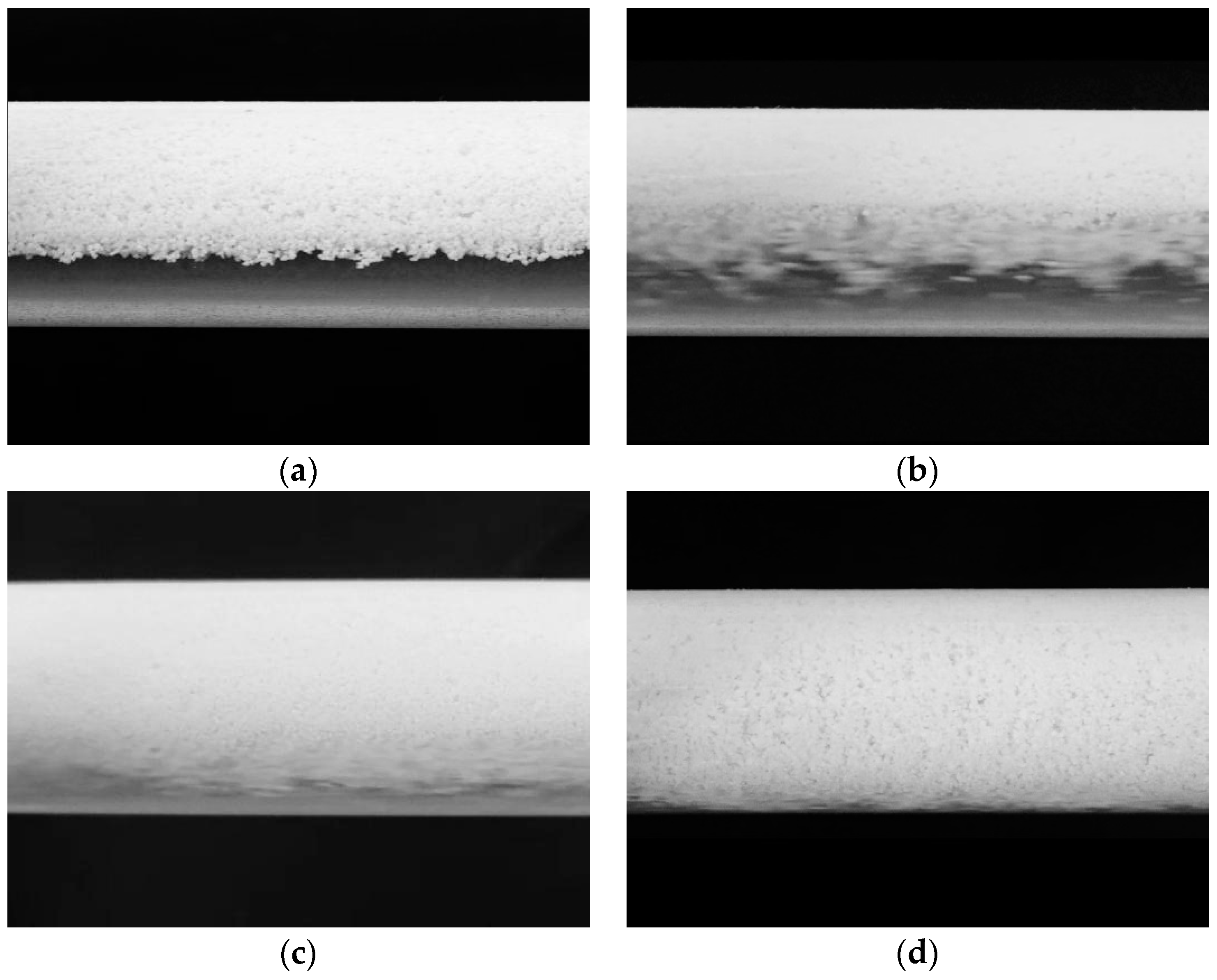
(1) Static bed (Figure 12a): In the case of a very small flow rate (or static state), polyethylene particles are gathered above the pipe due to their small density, and, at this time, it is difficult to reach the state of mixing of the two phases of the solid–liquid flow. Moreover, the flow velocity of the carrier fluid is not enough to drive the flow of the solid-phase particles, and the solid phase is basically static. This state cannot achieve the purpose of transporting particles. In particular, for ice slurry fluid with ice particles in the solid phase, particle agglomeration is bound to occur, resulting in clogging.

(2) Moving bed (Figure 12b): As the flow velocity increases, part of the particles gathered above the pipe converge into the carrier fluid and flow together, and the other part is gathered in the upper part of the pipe and flows slowly. In this flow state, the particles and the carrier fluid begin to mix and flow together, however, at this time, some of the particles will still float and agglomerate, resulting in high particle accumulation rates, slow flow velocity, low particle transport efficiency, and easy wear and clogging of the pipeline. In particular, for ice slurry fluids, an increase in the accumulation of ice particles still occurs, which in turn leads to ice blockage.

(3) Suspended bed (Figure 12c,d): With the further increase in flow velocity, the solid-phase particles gathered above the pipeline gradually converge into the entire area of the carrier fluid, according to whether the solid-phase particles are uniformly distributed can be divided into “non-homogenized suspended bed (Figure 12c)” and “homogenized suspended bed (Figure 12d).” In the suspended bed flow state, the particles are fully suspended, the solid phase follows the liquid phase together with the flow, which does not easily cause a clogging phenomenon, and is conducive to the safe, stable, and efficient transportation of slurry.

By comparing and analyzing the above four flow regimes, it can be found that, in order to ensure the safe and stable transport of the slurry, we should keep the slurry in the state of suspended bed, and the flow velocity cannot be too small. Therefore, it is necessary to find the velocity of the solid–liquid two-phase flow from the moving bed exactly transformed into a non-homogeneous suspended bed and the velocity that is the critical flow velocity.

4.2. Experimental Observations to Determine Critical Flow Velocity

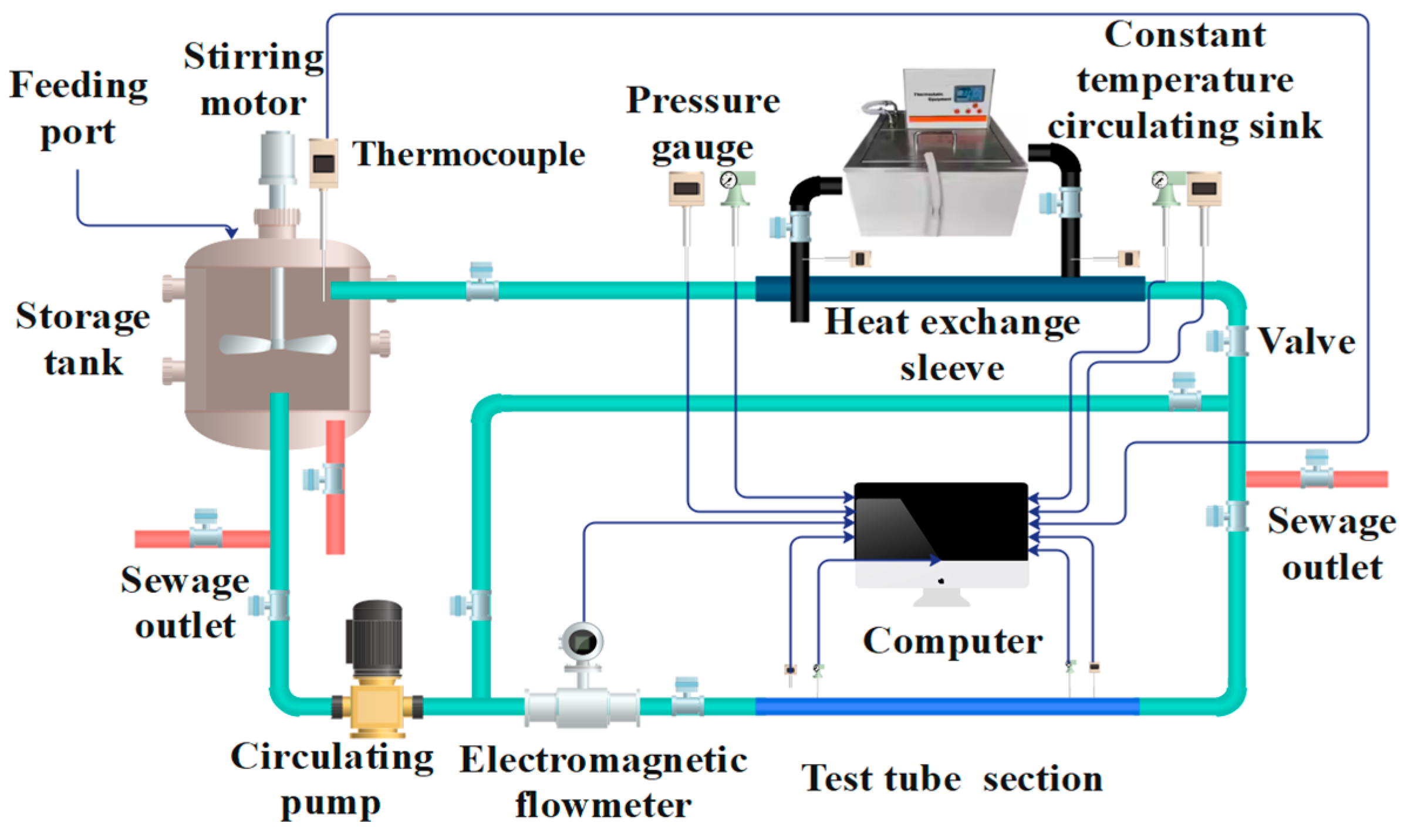
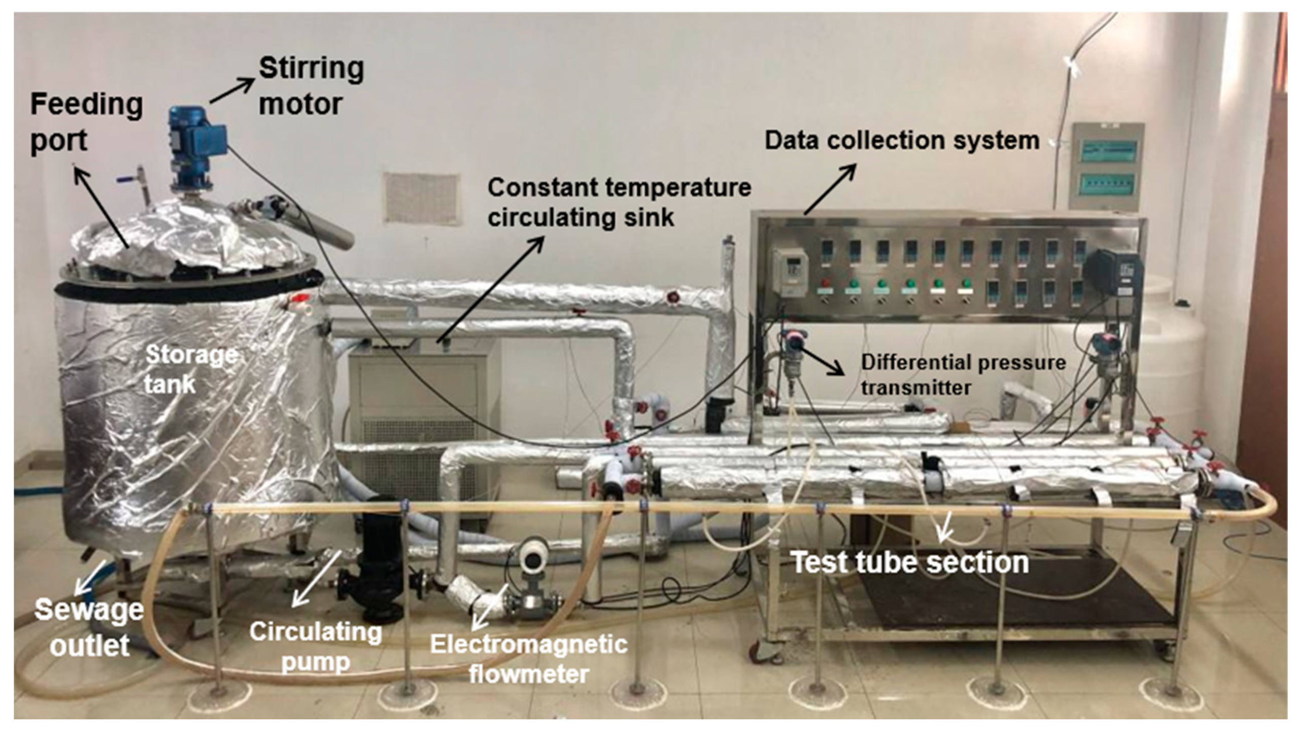
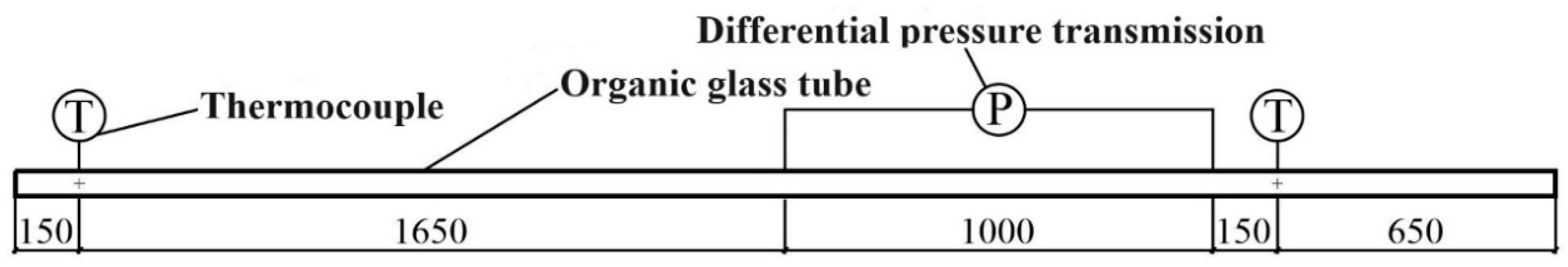
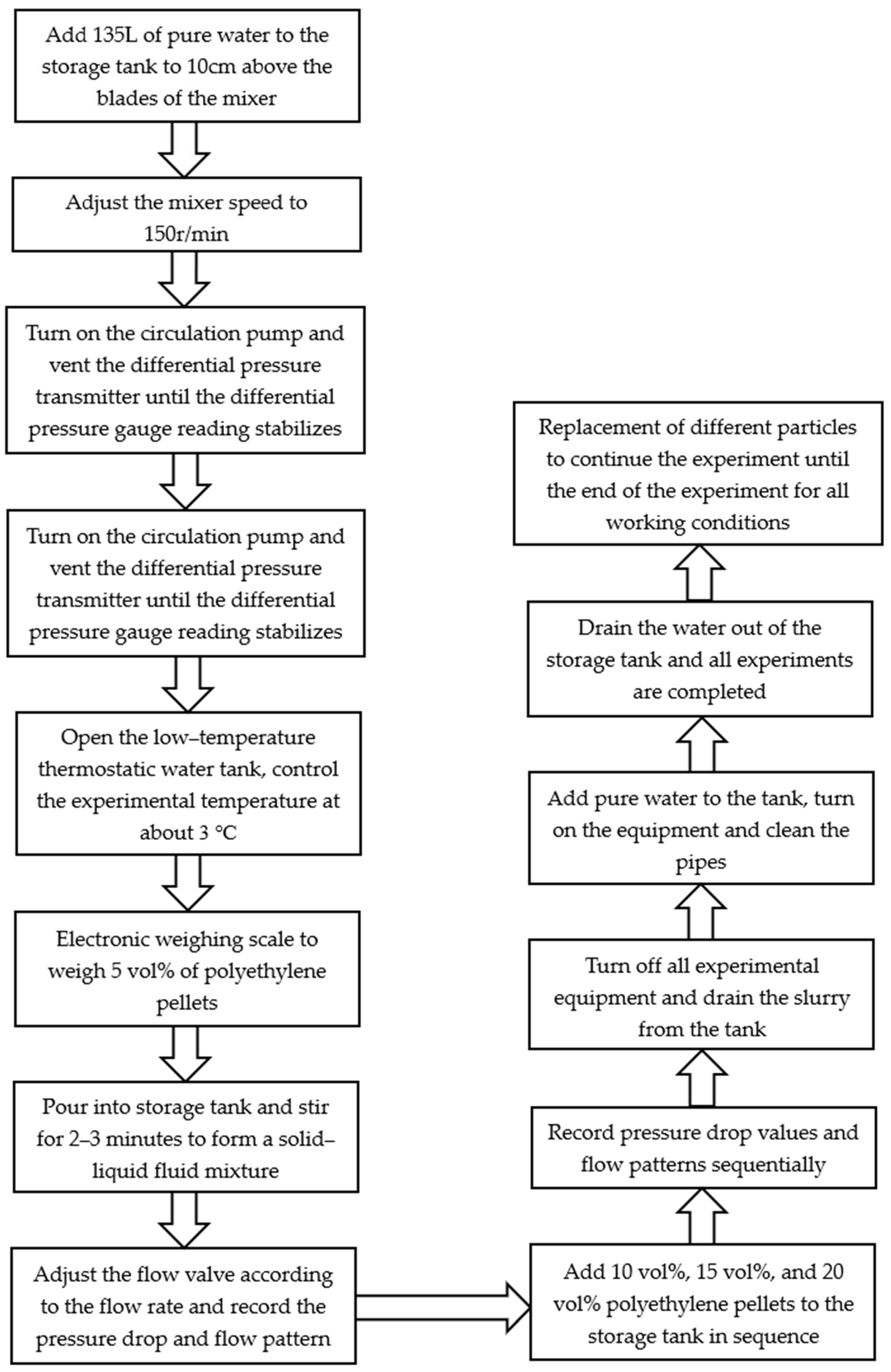
In order to determine the critical flow velocity, we first observe and record the flow pattern and pressure drop of the light particle slurry in the highly transparent Plexiglas tube (inner diameter 28 mm) by the observation method by using the experimental equipment and methods introduced in Section 2. The critical flow velocity intervals of the slurry under the corresponding working conditions can be found through the observation of its flow transition. The experimental conditions and flow patterns are shown in

Table 4. Observed flow patterns of slurry under different working conditions when the pipe diameter D = 28 mm.

	Cv	d = 0.3 mm				d = 0.4 mm				d = 0.5 mm
v (m/s)		5	10	15	20	5	10	15	20	5	10	15	20
0.1		②	②	①②	①	②	①	①	①	②	①②	①	①
0.2		②	②	②	②	②	②	②	①②	②	②	①②	①②
0.3		③	③	③	②	③	②	②	②	③	②	②	②
0.4		④	④	④	②	④	③	③	②	④	③	②	②
0.5		④	④	④	③	④	④	④	③	④	④	③	③
0.6		④	④	④	④	④	④	④	④	④	④	④	④
0.7		④	④	④	④	④	④	④	④	④	④	④	④
0.8		④	④	④	④	④	④	④	④	④	④	④	④
0.9		④	④	④	④	④	④	④	④	④	④	④	④
1		④	④	④	④	④	④	④	④	④	④	④	④

Note: ① Static bed; ② Moving bed; ③ Non-homogenized suspended bed; ④ Homogenized suspended bed. Solid content C_v in vol%.

.

In this table, with the increase in flow velocity, the velocity at the first appearance of the non-homogeneous suspended bed (identified as ③ in the table) can be regarded as the critical flow velocity under the experimental conditions. This value provides the computational basis for the numerical simulation method proposed below. Due to the visual error in visualizing the experimental observations, there is uncertainty in discriminating the morphology of the stationary and moving beds for mixed slurries at lower flow velocities. For example, in Table 4, when the solid-phase content C_v is 15% and the solid-phase particle size d = 0.3 mm, the phenomenon of both a static bed and moving bed (identified as ① and ② in the table, respectively) occurs when the flow velocity v = 0.1 m/s, in which one section of the test tube in the visualization experiment shows a static bed, while the other section shows a moving bed flow pattern. However, this phenomenon does not affect the observation of the inhomogeneous suspended bed or the determination of the critical flow velocity.

4.3. Numerical Simulation to Calculate the Critical Flow Velocity

The method of determining the critical flow velocity by experimentally observing the flow pattern is highly credible but time consuming and costly. Therefore, numerical simulation is a more efficient and economical prediction method. In addition, how to determine the moving bed and suspended bed and find out the critical flow velocity by numerical simulation is still a research problem. Here, we refer to the method proposed by Wasp [31]. The method is applied to the slurry flow model where the solid-phase density is greater than the liquid-phase density, and proposes the ratio of the solid-phase volume fraction vf at 0.08 times the pipe diameter below the top of the horizontal circular pipe to the volume fraction vf(y) at the center of the pipe as a criterion for judging, which is considered to be a suspended bed when vf/vf(y) > 0.8. However, for the solid–liquid two-phase flow of ice-slurry-type light particles with solid-phase density less than liquid-phase density, no relevant reports on the calculation of critical flow velocity similar to the concentration distribution method have been seen.

We carefully observe the flow characteristics of the static bed, moving bed, non-homogenized suspended bed, and homogenized suspended bed in Figure 12, as follows: (1) in the static bed, the particles are gathered above the pipe; (2) in the moving bed, some of the particles converge into the carrier fluid and flow together, and the other part is gathered in the upper part of the pipe and flows slowly; (3) in the non-homogenized suspended bed, the solid-phase particles converge into the whole area of the carrier fluid gradually, but are still densely packed on the top and not at all on the bottom; and (4) in the homogenized suspended bed, the solid-phase particles are uniformly distributed throughout the region. Therefore, the concentration distribution of solid-phase particles can be used to characterize the flow. Accordingly, we propose the concentration distribution method for calculating the critical flow velocity of light particle solid–liquid two-phase flow. The velocity of light particle slurry is recognized as the critical flow velocity when the ratio of the solid phase volume fraction vf is 0.08 times the diameter of the pipe above the bottom of the pipe to the solid phase volume fraction vf(y) at the center of the pipe vf/vf(y) = 0.75. The selection of the location of the feature 0.08 times that of the pipe diameter above the bottom of the pipe was based on selecting the region close to the bottom of the pipe and avoiding the boundary layer. In addition, in vf/vf(y) = 0.75, the value of 0.75 is determined by comparing and verifying the critical flow rate obtained using the concentration distribution method (numerical simulation to obtain the volume fraction of the solid phase), with the critical flow velocity being obtained by the experimental observation method shown in Section 4.1. The specific working conditions for the numerical simulation are shown in

Table 5. Specific working conditions for numerical simulation.

Name	Working Condition Parameters
Pipe diameter: D/mm	17, 24, 28
Solid particle size: d/mm	0.3, 0.4, 0.5
Flow velocity: v/m·s−1	0.1–1.0 (Interval 0.01 m/s)
Solid content (IPF): Cv vol%	5, 10, 15, 20
vf/vf(y)	0.6, 0.7, 0.75, 0.8, 0.85, 0.9

, and the concentration distribution method is specified as follows:

(1) Using the numerical simulation method introduced in the third section, numerical simulation is performed on the experimental conditions mentioned in Table 4 (flow velocity interval is 0.01 m/s), and the solid phase volume fraction in the horizontal circular tube is obtained. For the entire horizontal circular pipe, we extract the solid phase volume fraction value of the characteristic point, that is, the solid phase volume fraction vf at 0.08 times that of the pipe diameter above the bottom of the pipe and the solid phase volume fraction vf(y) at the center of the pipe.

(2) The assumed flow velocity of the slurry when vf/vf(y) is equal to 0.6, 0.7, 0.75, 0.8, 0.85, and 0.9 is assumed to be the critical flow velocity to obtain the assumed flow velocity derived from the concentration distribution method, respectively, and the values are summarized in

Table 6. Slurry critical velocity (m/s) under different working conditions obtained by the concentration distribution method when the pipe diameter D = 28 mm.

	Cv	d = 0.3 mm				d = 0.4 mm				d = 0.5 mm
v f/vf(y)		5	10	15	20	5	10	15	20	5	10	15	20
0.60		0.25	0.26	0.30	0.36	0.27	0.32	0.38	0.41	0.3	0.41	0.46	0.50
0.70		0.28	0.33	0.34	0.43	0.29	0.33	0.41	0.50	0.32	0.45	0.51	0.55
0.75		0.30	0.32	0.35	0.46	0.32	0.36	0.43	0.53	0.34	0.49	0.55	0.58
0.80		0.34	0.35	0.38	0.51	0.36	0.42	0.50	0.56	0.39	0.53	0.60	0.62
0.85		0.36	0.37	0.41	0.53	0.39	0.44	0.53	0.57	0.42	0.56	0.62	0.63
0.90		0.37	0.39	0.42	0.54	0.41	0.46	0.56	0.60	0.44	0.59	0.64	0.65
Experimental observation		0.3	0.3	0.3	0.5	0.3	0.4	0.4	0.5	0.3	0.4	0.5	0.5

Note: In the table, the values in red font are those that differ significantly from the critical flow rate obtained by the experimental observation method, and the values in blue font are those that are closer to the critical flow rate obtained by the experimental observation method.

. For comparison, the critical flow velocity obtained using the experimental observation method is also shown in the last row of the table. Since the slurry flow velocity interval is 0.1 m/s in the experiment, the critical flow velocity obtained using the experimental observation method has some errors.

(3) The results obtained from the concentration distribution method in Table 6 are compared with the critical flow velocity derived from the experimental observation method. The larger differences in values are shown in red. It can be found that, at vf/vf(y) = 0.75, the concentration distribution method is closest to the results of the experimental observation method, and, therefore, a final value of 0.75 is determined.

According to Table 6, the concentration distribution method matches the experimental results with high accuracy at tube diameter D = 28 mm and particle diameters d = 0.3 mm and 0.4 mm, while the deviation is larger at particle diameter d = 0.5 mm and solid-phase content C_v of 10 vol% and 20 vol%. In view of the experimental slurry flow rate interval of 0.1 m/s, the value is still within a reasonable range. Accordingly, it can be shown that our proposed concentration distribution method for solid–liquid two-phase flow of ice-slurry-type light particles can calculate the critical flow velocity more accurately.

4.4. Effect of Flow Pattern on Pressure Drop

Through experiments or numerical simulations, we have identified the minimum flow velocity, that is, the critical flow velocity, for the safe and energy-efficient transport of light particle slurries. However, when the flow velocity is larger than the critical flow velocity, what is the effect on the slurry transport when the flow velocity continues to increase? When the slurry is in the state of a homogeneous suspended bed and we continue to increase the flow velocity, the flow characteristics of the slurry do not change significantly. Continuing to increase the flow velocity, on the one hand, increases the efficiency of solid-phase transport per unit time, but, at the same time, it will also increase the transport cost and increase the erosion of the slurry on the pipeline.

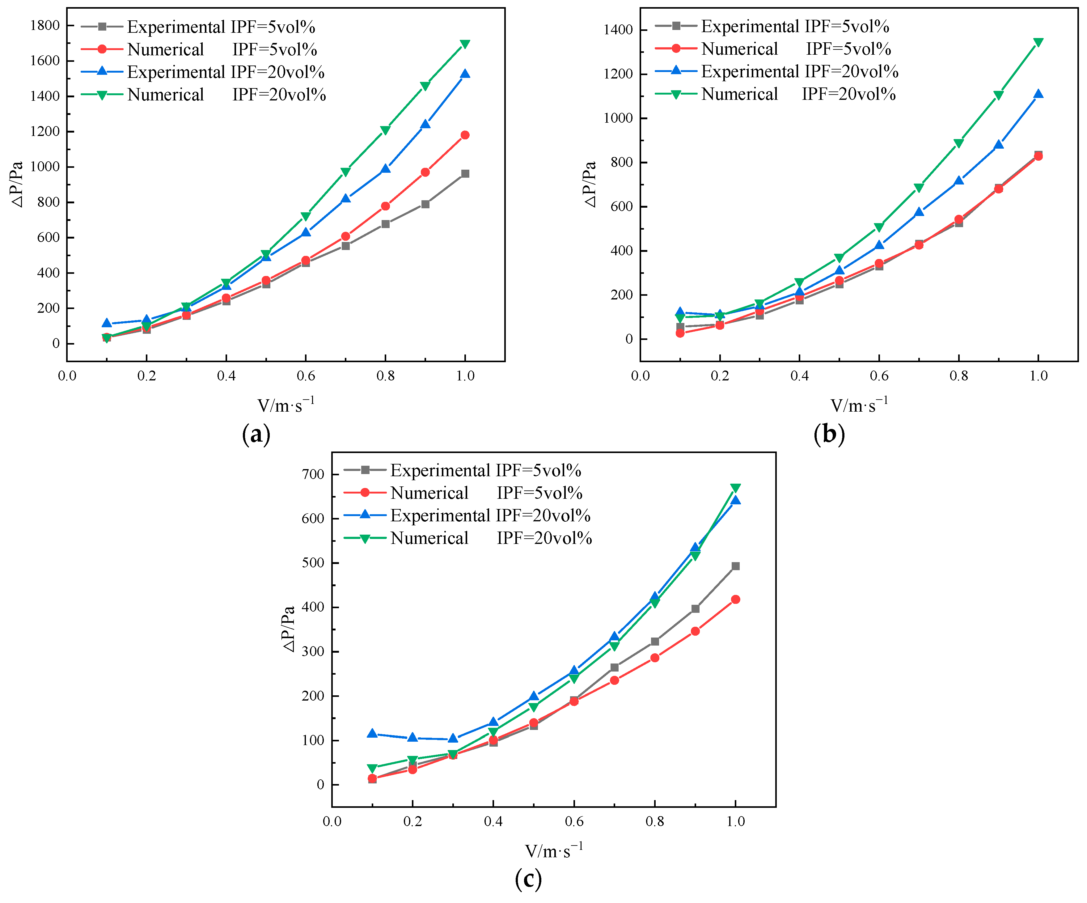
Figure 13 shows the values of pressure drop recorded in the experiment where the experimental observation method was carried out to determine the critical flow velocity. Comparing the pressure drop data in Figure 13 with the flow patterns in Table 4, the following can be observed: (1) When the slurry is in a static bed and a moving bed, and transitioning to a non-homogeneous suspended bed, the pressure drop of the slurry increases slowly, and even decreases with increasing flow velocity. This is the case when energy-saving transport is very favorable. (2) After the slurry is in a suspended bed, continuing to increase the flow velocity, the pressure drop of the slurry will increase rapidly. Therefore, the critical flow velocity when the slurry reaches the non-homogeneous suspended bed is favorable for energy-saving transportation, and continuing to increase the flow velocity will significantly increase the transportation cost.

4.5. Effect of Solid-Phase Content and Particle Size on Critical Flow Velocity

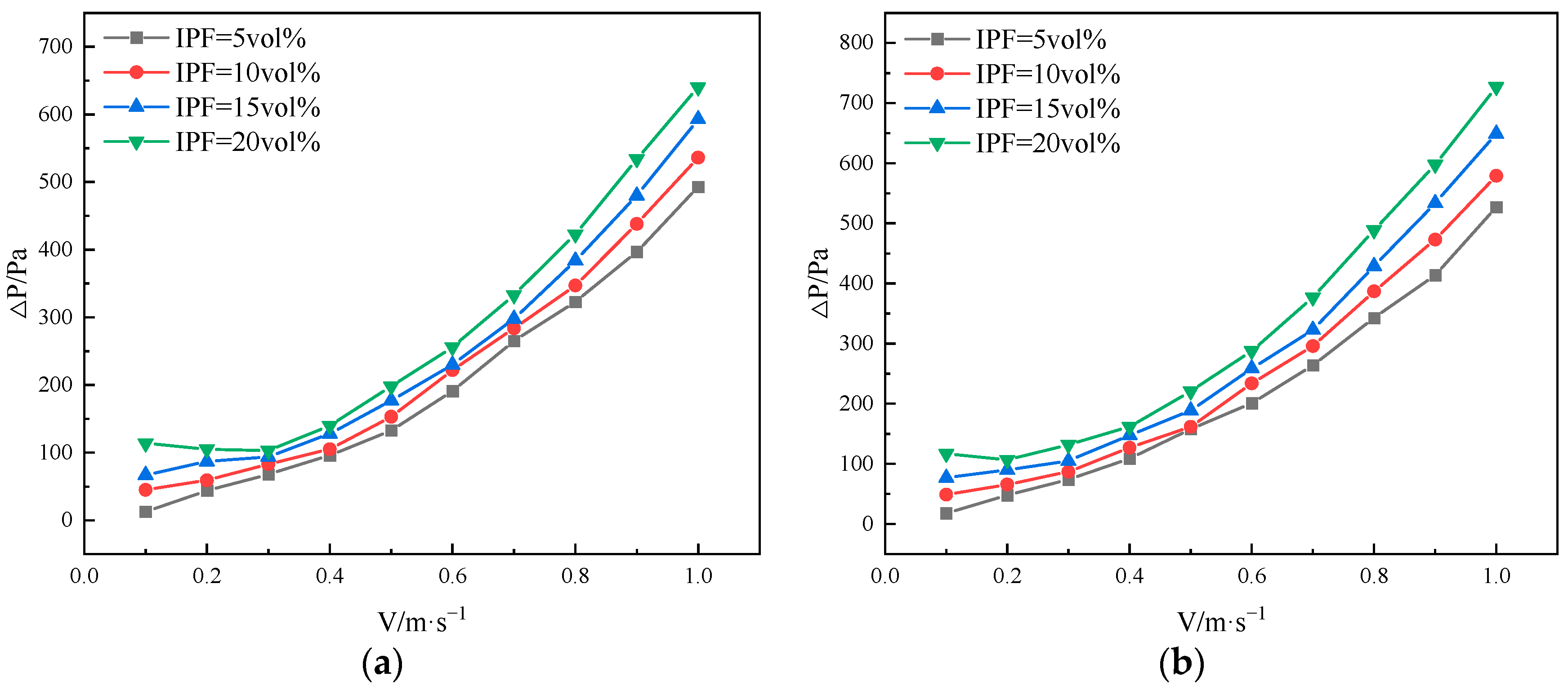
A numerical simulation of the flow of light particle slurry (solid phase is polyethylene particles) in a horizontal circular pipe with pipe diameters D = 28 mm and 17 mm; particle diameters d = 0.3 mm, 0.4 mm, and 0.5 mm; and solid-phase content C_v = 5 vol%, 10 vol%, 15 vol%, and 20 vol% is carried out. The critical flow velocity for each condition is obtained using the concentration distribution method and the results are organized in Figure 14. It can be found that the critical flow velocity increases with the increase in solid-phase content under the simulated conditions. This is because the increase in solid-phase content of the light particle slurry inhibits the turbulence intensity, weakens the support of the carrier fluid on the solid-phase particles, and requires an increase in the flow velocity to maintain a certain degree of turbulence intensity [32]. At the same time, the increase in solid-phase content makes the viscosity of the light particle slurry increase, and the solid-phase particles are more tightly bonded to each other; moreover, due to the existence of the difference in the densities between the two phases, a tendency to upward movement occurs, and a larger flow velocity is required in order to maintain the state of the suspended bed, therefore, the critical flow velocity will also be increased. This is in agreement with the conclusion obtained by Rawat [15].

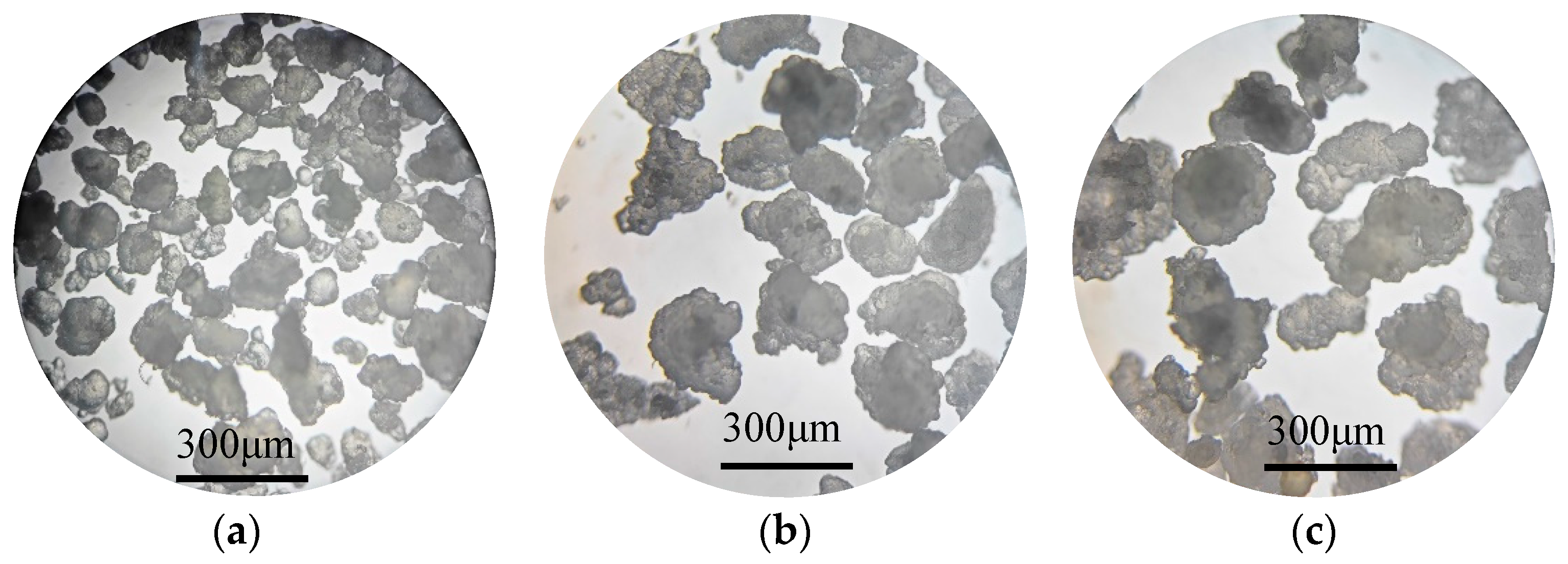
It can also be observed in Figure 14 that the critical flow velocity increases with the increase in the solid-phase particle size under the simulated conditions. This is because, on the one hand, solid-phase particles with larger particle sizes are subjected to larger buoyancy and inertia forces, and larger flow velocities are required to suppress these two forces. On the other hand, however, the larger the solid-phase particles are, the larger the area of action of drag force exerted on the particles, and the drag force required to keep them in motion increases, therefore, larger flow velocities are required to make the light-particle slurry exhibit a suspended-bed flow. This is more consistent with the conclusions of Tian [21], but he believes that the increase in additive concentration during ice production leads to a decrease in the density difference between the solid–liquid two-phase, which also affects the determination of the critical flow velocity. However, in this paper, the selection of polyethylene particles as the solid phase does not have the time-dependent behavior of ice-crystalline particles, does not occur in the ice-crystalline particles of melting and agglomeration, and is able to always maintain a constant particle size, while the density of slurry is unchanged, which allows for a more accurate determination of critical flow velocity [33]. It is also found that the critical flow velocities of the three particle sizes are close to each other when the solid-phase content is 5 vol%, as shown in Figure 12a, which are 0.34 m/s, 0.36 m/s, and 0.39 m/s, respectively. This is due to the fact that when the solid-phase content is lower, the solid-phase particles are more dispersed in the pipeline, and the denseness of the solid-phase particles is more in play, which makes the effect of the size of the solid-phase particles on the critical flow velocity weaker.

5. Conclusions and Outlook

5.1. Conclusions

In order to find the optimal flow velocity for the safe and energy-saving transportation of ice-slurry-type light particle slurries, this paper investigates the critical flow velocity of light particle slurries (consisting of polyethylene particles and water with a density of 922 kg/m³) flowing in a horizontal circular pipe by means of experimental and numerical simulation methods. The main conclusions drawn are as follows:

(1) The flow velocity for safe and energy-saving transportation of light particle slurries is recommended to be its critical flow velocity. When the flow velocity is lower than the critical flow velocity, the particles pile up above the pipeline and cannot follow the flow of the liquid phase, so the transportation efficiency is low easily clogged; moreover, when the flow velocity is higher than the critical flow velocity, the transportation cost will be increased significantly.

(2) The critical flow velocities of the slurry under different working conditions were derived using the experimental observation method. The experimental conditions were pipe diameter D = 28 mm; particle diameters d = 0.3 mm, 0.4 mm, and 0.5 mm; solid-phase content C_v = 5 vol%, 10 vol%, 15 vol%, and 20 vol%; and slurry flow velocity v in the range of 0.1~1 m/s (interval 0.1 m/s).

(3) A new concentration distribution method for the critical flow velocity of ice-slurry-type light particle slurries is first proposed, and the velocity of light particle slurries is recognized as the critical flow velocity when the ratio of the solid-phase volume fraction vf at a location of 0.08 D above the bottom of the pipe to the solid-phase volume fraction vf(y) at the center of the pipe vf/vf(y) = 0.75. The solid phase volume fraction was obtained by an experimentally validated numerical simulation method. By comparing the critical flow velocity obtained by the experimentally observed method, it can be found that the concentration distribution method has a high accuracy. Thus, the concentration distribution method can be used to obtain the critical flow velocity under different operating conditions simply and economically by numerical simulation.

(4) The experimental and numerical simulation results show that the increase in solid-phase content and particle size will lead to the increase in critical flow velocity under the condition that the other parameters remain unchanged. In the actual transportation process, the selection of a smaller particle size is more conducive to the energy-saving transportation of light particle slurry; moreover, especially for ice slurry, a smaller particle size is also more conducive to the safe transportation of slurry.

5.2. Outlook

(1) The new concentration distribution method based on numerical simulation to study the critical flow rate proposed in this paper is mainly for horizontal circular pipes, while the applicability to special pipes, such as curved pipes, needs to be further investigated.

(2) In this study, polyethylene particles were used instead of ice-crystal particles for particle flow characterization, ignoring the influence of the kinetic behavior between ice-crystal particles on the flow characteristics of the slurry, which needs to be explored in depth in future studies.

References

1. Long, Y.; Wang, S.; Wang, J.; Zhang, T. Numerical and analytical investigations of heat transfer for a finned tube heat exchanger with ice slurry as cooling medium. Sci. Technol. Built Environ. 2017, 23, 478–489. [Google Scholar] [CrossRef]
2. Kalaiselvam, S.; Karthik, P.; Ranjit, P.S. Numerical investigation of heat transfer and pressure drop characteristics of tube–fin heat exchangers in ice slurry HVAC system. Appl. Therm. Eng. 2009, 29, 1831–1839. [Google Scholar] [CrossRef]
3. Kauffeld, M.; Gund, S. Ice slurry–History, current technologies and future developments. Int. J. Refrig. 2019, 99, 264–271. [Google Scholar] [CrossRef]
4. Kauffeld, M.; Wang, M.J.; Goldstein, V.; Kasza, K.E. Ice slurry applications. Int. J. Refrig. 2010, 33, 1491–1505. [Google Scholar] [CrossRef]
5. Saboorian-Jooybari, H.; Dejam, M.; Chen, Z. Heavy oil polymer flooding from laboratory core floods to pilot tests and field applications: Half-century studies. J. Pet. Sci. Eng. 2016, 142, 85–100. [Google Scholar] [CrossRef]
6. Liu, X.Y.; Li, Y.H.; Li, X.Q.; Zhao, C.C.; Liu, L.J. Glled Crude Oil Particle Deformation under Hydraulic Suspension Transport Investigated by Numerical Simulation. Adv. Mater. Res. 2014, 900, 757–760. [Google Scholar] [CrossRef]
7. Thakur, A.K.; Kumar, R.; Banerjee, N.; Chaudhari, P.; Gaurav, G.K. Hydrodynamic modeling of liquid-solid flow in polyolefin slurry reactors using CFD techniques-A critical analysis. Powder Technol. 2022, 405, 117544. [Google Scholar] [CrossRef]
8. Okamoto, Y.; Mine, Y.; Wada, D.; Umakoshi, H. Development of Easy, Harmless, and Energy-saving Water Cleanup Method Based on Self-flotation of Hollow Glass Beads Coated with Fatty Acids. Chem. Lett. 2016, 45, 544–546. [Google Scholar] [CrossRef]
9. Ni, G.; Fu, Z.; Li, Z.; Sun, G.; Zhang, X.; Wang, G.; Wang, Z.; Liu, Y.; Xu, C. Performance study of new lightweight cementitious composites with glass beads as filler. J. Build. Eng. 2024, 90, 109477. [Google Scholar] [CrossRef]
10. Cunliffe, C.J.; Dodds, J.M.; Dennis, D. Flow correlations and transport behavior of turbulent slurries in partially filled pipes. Chem. Eng. Sci. 2021, 235, 116465. [Google Scholar] [CrossRef]
11. Harbottle, D.; Fairweather, M.; Biggs, S. The minimum transport velocity of colloidal silica suspensions. Chem. Eng. Sci. 2011, 66, 2309–2316. [Google Scholar] [CrossRef]
12. Januário, J.R.; Maia, C.B. CFD-DEM Simulation to Predict the Critical Velocity of Slurry Flows. J. Appl. Fluid Mech. 2020, 13, 161–168. [Google Scholar] [CrossRef]
13. Wang, Z.B.; Zheng, Y.G. Critical flow velocity phenomenon in erosion-corrosion of pipelines: Determination methods, mechanisms and applications. J. Pipeline Sci. Eng. 2021, 1, 63–73. [Google Scholar] [CrossRef]
14. Doron, P.; Barnea, D. A three-layer model for solid-liquid flow in horizontal pipes. Int. J. Multiph. Flow 1993, 19, 1029–1043. [Google Scholar] [CrossRef]
15. Rawat, K.S.; Verma, A.; Pratihar, A.K.; Singh, A.K.; Maheshwari, P. Numerical Investigation on Critical Velocity of Ice Slurry Flow. IOP Conf. Ser. Mater. Sci. Eng. 2020, 802, 012002. [Google Scholar] [CrossRef]
16. Kitanovski, A.; Vuarnoz, D.; Ata-Caesar, D.; Egolf, P.W.; Hansen, T.M.; Doetsch, C. The fluid dynamics of ice slurry. Int. J. Refrig. 2005, 28, 37–50. [Google Scholar] [CrossRef]
17. Azamathulla, H.M.; Ahmad, Z. Estimation of Critical Velocity for Slurry Transport through Pipeline Using Adaptive Neuro-Fuzzy Interference System and Gene-Expression Programming. J. Pipeline Syst. Eng. Pract. 2013, 4, 131–137. [Google Scholar] [CrossRef]
18. Kökpınar, M.A.; Göğüs, M. Critical flow velocity in slurry transporting horizontal pipelines. J. Hydrol. Eng. 2001, 127, 763–771. [Google Scholar] [CrossRef]
19. Shook, C.A.; Roco, M.C. Critical deposit velocity in slurry flow. AICHE J. 1985, 31, 1401–1404. [Google Scholar]
20. Rawat, K.S.; Pratihar, A.K. Numerical Investigation of Ice Slurry Flow in a Horizontal Pipe. IOP Conf. Ser. Mater. Sci. Eng. 2018, 310, 012095. [Google Scholar] [CrossRef]
21. Tian, Q.; He, G.; Wang, H.; Cai, D. Simulation on transportation safety of ice slurry in ice cooling system of buildings. Energy Build. 2014, 2, 262–270. [Google Scholar] [CrossRef]
22. Wu, T.; Zhu, N.; Hu, Z.G.; Luo, Z.Y.; Hu, P.F.; Lei, F. Numerical study on critical flow velocity of ice slurry in the pipe of ice source heat pump system. Energy Built Environ. 2023, 5, 607–614. [Google Scholar] [CrossRef]
23. Rayhan, F.A.; Rizal, R. Pressure drop and non-Newtonian behavior of ice slurry in a horizontal pipe. J. Braz. Soc. Mech. Sci. Eng. 2022, 44, 5. [Google Scholar] [CrossRef]
24. Qin, Z.; Huang, W.; Ning, Z.; Hu, K. Exchange Flows in Inclined Pipes with Different Viscosity Ratios. Appl. Sci. 2024, 14, 1573. [Google Scholar] [CrossRef]
25. Kitanovski, A.; Poredo, A. Concentration distribution and viscosity of ice-slurry in heterogeneous flow. Int. J. Refrig. 2002, 25, 827–835. [Google Scholar] [CrossRef]
26. Frei, B.; Egolf, P.W. Viscometry applied to the Bingham Substance Ice Slurry. In Proceedings of the Second Workshop on Ice Slurries of the International Institute of Refrigeration, Paris, France, 25–26 May 2000; pp. 48–59. [Google Scholar]
27. Arellano, M.; Benkhelifa, H.; Alvarez, G.; Flick, D. Coupling population balance and residence time distribution for the ice crystallization modeling in a scraped surface heat exchanger. Chem. Eng. Sci. 2013, 102, 502–513. [Google Scholar] [CrossRef]
28. Ekambara, K.; Sanders, R.S.; Nandakumar, K.; Masliyah, J.H. Hydrodynamic Simulation of Horizontal Slurry Pipeline Flow Using ANSYS-CFX. Ind. Eng. Chem. Res. 2009, 48, 8159–8171. [Google Scholar] [CrossRef]
29. Vuarnoz, D.; Sari, O.; Egolf, P.W.; Liardon, H. Ultrasonic velocity profiler UVP-XW for ice-slurry flow characterization. In Proceedings of the Third International Symposium on Ultrasonic Doppler Methods for Fluid Mechanics and Fluid Engineering, Lausanne, Switzerland, 9–11 September 2002. [Google Scholar]
30. Wang, J.H.; Zhang, T.F.; Wang, S.G. Heterogeneous ice slurry flow and concentration distribution in horizontal pipes. Int. J. Heat Fluid Flow 2013, 44, 425–434. [Google Scholar] [CrossRef]
31. Wasp, E.J. Solid-Liquid Flow Slurry Pipeline Transportation; Trans Tech Publications: Clausthal, Germany, 1977. [Google Scholar]
32. Grozdek, M.; Khodabandeh, R.; Lundqvist, P. Experimental investigation of ice slurry flow pressure drop in horizontal tubes. Exp. Therm. Fluid Sci. 2009, 33, 357–370. [Google Scholar] [CrossRef]
33. Kumano, H.; Hirata, T.; Hagiwara, Y.; Tamura, F. Effects of storage on flow and heat transfer characteristics of ice slurry. Int. J. Refrig. 2012, 35, 122–129. [Google Scholar] [CrossRef]
Figure 1. Schematic diagram of the experimental setup.
Applsci 14 06313 g001
Figure 2. Physical diagram of the experimental setup.
Applsci 14 06313 g002
Figure 3. Schematic diagram of test pipe section.
Applsci 14 06313 g003
Figure 4. Three kinds of polyethylene particle: (a) 0.3 mm; (b) 0.4 mm; (c) 0.5 mm.
Applsci 14 06313 g004
Figure 5. Flow chart of the experimental method.
Applsci 14 06313 g005
Figure 6. Meshing: (a) Inlet and outlet grid; (b) Wall grid.
Applsci 14 06313 g006
Figure 7. Flow of numerical simulation run.
Applsci 14 06313 g007
Figure 8. Effect of different numbers of grids on particle concentration distribution.
Applsci 14 06313 g008
Figure 9. Comparison of pressure drop between experimental and simulated values under different operating conditions: (a) D = 17 mm, d = 0.3 mm; (b) D = 24 mm, d = 0.5 mm; (c) D = 28 mm, d = 0.4 mm.
Applsci 14 06313 g009
Figure 10. Comparison of simulated and experimental values of velocity field.
Applsci 14 06313 g010
Figure 11. Comparison of simulated and experimental values of pressure drop.
Applsci 14 06313 g011
Figure 12. Flow pattern of mixed slurry: (a) Static bed; (b) Moving bed; (c) Non-homogenized suspended bed; (d) Homogenized suspended bed.
Applsci 14 06313 g012
Figure 13. Variation of pressure drop with flow velocity: (a) d = 0.3 mm; (b) d = 0.4 mm.
Applsci 14 06313 g013
Figure 14. Variation of critical flow velocity with solid-phase content and particle size: (a) D = 28 mm; (b) D = 17 mm.
Applsci 14 06313 g014