Article

A 1D Convolutional Neural Network (1D-CNN) Temporal Filter for Atmospheric Variability: Reducing the Sensitivity of Filtering Accuracy to Missing Data Points

1
Faculty of Data Science, City University of Macau, Macau 999078, China
2
Guangzhou Institute of Tropical and Marine Meteorology/Guangdong Provincial Key Laboratory of Regional Numerical Weather Prediction, China Meteorological Administration, Guangzhou 510000, China
3
Hong Kong Observatory, 134A Nathan Road, Kowloon, Hong Kong, China
4
ESCAP/WMO Typhoon Committee Secretariat, Macau 999078, China
5
Japan Agency for Marine-Earth Science and Technology, Kanazawa District, Yokohama 236-0001, Japan
6
College of Meteorology and Oceanography, National University of Defense Technology, Changsha 410073, China
7
College of Atmospheric Sciences, Lanzhou University, Lanzhou 730000, China
*
Authors to whom correspondence should be addressed.
Appl. Sci. 2024, 14(14), 6289; https://doi.org/10.3390/app14146289
Submission received: 26 June 2024 / Revised: 16 July 2024 / Accepted: 17 July 2024 / Published: 19 July 2024
(This article belongs to the Special Issue Machine Learning Approaches for Geophysical Data Analysis)

Abstract

:
The atmosphere exhibits variability across different time scales. Currently, in the field of atmospheric science, statistical filtering is one of the most widely used methods for extracting signals on certain time scales. However, signal extraction based on traditional statistical filters may be sensitive to missing data points, which are particularly common in meteorological data. To address this issue, this study applies a new type of temporal filters based on a one-dimensional convolution neural network (1D-CNN) and examines its performance on reducing such uncertainties. As an example, we investigate the advantages of a 1D-CNN bandpass filter in extracting quasi-biweekly-to-intraseasonal signals (10–60 days) from temperature data provided by the Hong Kong Observatory. The results show that the 1D-CNN achieves accuracies similar to a 121-point Lanczos filter. In addition, the 1D-CNN filter allows a maximum of 10 missing data points within the 60-point window length, while keeping its accuracy higher than 80% (R2 > 0.8). This indicates that the 1D-CNN model works well even when missing data points exist in the time series. This study highlights another potential for applying machine learning algorithms in atmospheric and climate research, which will be useful for future research involving incomplete time series and real-time filtering.

1. Introduction

The atmospheric system exhibits characteristics and patterns of different time scales, ranging from hours to years. For instance, synoptic scale systems, which have typical 1–7-day cycles, are primary drivers of daily weather patterns [1,2,3,4]. Seasonal variability, spanning 4–12 months, reflects the primary signals of seasonal changes and the annual cycle [5,6,7,8]. The El Niño/Southern Oscillation (ENSO), with 2–7-year cycles, is one of the main drivers of global climate variability on an interannual time scale on an annual basis [9,10,11,12]. In particular, the quasi-biweekly oscillation (QBWO, 10–20 days) and intraseasonal oscillation (ISO, 30–90 days) serve as the bridge linking low-frequency climate variability with synoptic weather systems. They are also critical for improving the accuracy of short- and medium-term climate predictions [13,14,15,16].
When studying different atmospheric variabilities, statistical temporal filters are a common way to extract signals on certain time scales. For example, the running average is one of the simplest ways to smooth out high-frequency signals, such as interannual variability, in climate research [17,18]. The Fast Fourier Transform (FFT) filter is another widely used method to extract periodic signals [19,20]. In particular, for intraseasonal signal detection, Butterworth [21] and Lanczos [22] bandpass filters are often utilized to extract intraseasonal variability and have been applied to studies on boreal summer intraseasonal oscillation [23,24], Madden–Julian Oscillation (MJO) [25,26], QBWO [27,28,29], etc. Moreover, sharp bandpass filters were also utilized by Zhang et al. [30] to distinguish QBWO and ISO signals from the daily outgoing longwave radiation input.
Among these statistical filters, the Lanczos filter is one of the most popular bandpass filters for identifying signals on quasi-biweekly and intraseasonal time scales. It has been reported that the Lanczos filter could reduce aliasing artifacts by suppressing high-frequency components, which are often evident in other filters such as the FFT filter, during filtering calculations. The Lanczos filter is also known to be able to reduce artificial oscillations caused by abrupt changes that may exist in the input series [31], which is often observed in the atmospheric system [32,33]. On the other hand, the shortcomings of the Lanczos filter are also obvious. The Lanczos filter has edge effects when processing the beginning and end of the dataset [34]. Because the Lanczos filter relies on a certain number of neighboring data points to calculate the output value of each point, there may be loss of data at the very beginning and the end of the filtered output, depending on the length of the window applied. Due to the same reason, the filter may be unable to work properly if missing values exist in the input time series, and this will result in no valid output values near the missing values. Since incomplete time series are a common and unavoidable issue in meteorological data, especially for in situ observations, it remains a challenge to extract QBWO and ISO signals from station data by utilizing the Lanczos filter. These shortcomings of the Lanczos filter also exist in most statistical filtering methods.
Aiming at addressing the above challenges of statistical temporal filters, this study introduces and employs a new type of filtering approach based on machine learning tools, or more specifically, a one-dimensional convolutional neural network (1D-CNN) [34,35,36]. Focus is particularly put on bandpass filtering due to its broad application in studies on QBWO and ISO, which serve as important atmospheric signals affecting weather variability worldwide [13], but the findings also hold for highpass and lowpass filters. In a recent study, Stan and Mantripragada [34] proposed and showed that a CNN-based filter can be applied to time series with lengths comparable to the period of the signal being extracted. This implies that the CNN training process could ensure that CNN-based filters capture accurate enough signals without considering neighboring data points. In this sense, CNN-based filters may also reduce filtering uncertainties due to missing data points, as mentioned above. However, this has not been studied in previous research. It remains unclear whether CNN-based filters work well for discontinuous time series. Thus, in this study, with a detailed explanation about the procedure of constructing a 1D-CNN filter, we examine how a 1D-CNN filter can be utilized to address the challenges in filtering time series with missing values.
Quasi-biweekly-to-intraseasonal variability is one of the important atmospheric signals affecting South China and Hong Kong [37], so we take meteorological station observations from the Hong Kong Observatory as sample data. The rest of this article is structured as follows: Section 2 introduces the datasets, analysis methods, and evaluation indicators used in the study; Section 3 and Section 4 explain the construction process of the 1D-CNN filter and its validity; Section 5 discusses the advantages of the 1D-CNN bandpass filter in dealing with incomplete time series; finally, Section 6 summarizes the key findings of the study and discusses them.

2. Data and Methods

2.1. Data

The Hong Kong Observatory collects data on nearly 100 automatic weather stations, including data on surface air temperature, wind speed, wind direction, rainfall, etc. The data utilized in this article include the daily average temperature, daily maximum temperature, and daily minimum temperature data of the 14 sites: Ta Kwu Ling (TKL), Lau Fau Shan (LFS), Wetland Park (WLP), Shek Kong (SEK), Tai Mo Shan (TMS), Sha Tin (SHA), Tate’s Cairn (TC), King’s Park (KP), Hong Kong International Airport (HKA), Hong Kong Observatory (HKO), Sha Lo Wan (SLW), Peng Chau (PEN), Cheung Chau (CCH), and Waglan Island (WGL) (Table 1). For simplicity, in the following discussion, we refer temperature to as surface air temperature, unless otherwise specified.
The temperature data of these stations contain missing data points (Table 1), which implies difficulties for extracting target signals by using the Lanczos filter or other commonly used filters. Table 1 lists the 14 sites selected for this article, their position, the number of missing values for daily means, and the maximum and minimum temperatures, respectively.

2.2. Methods

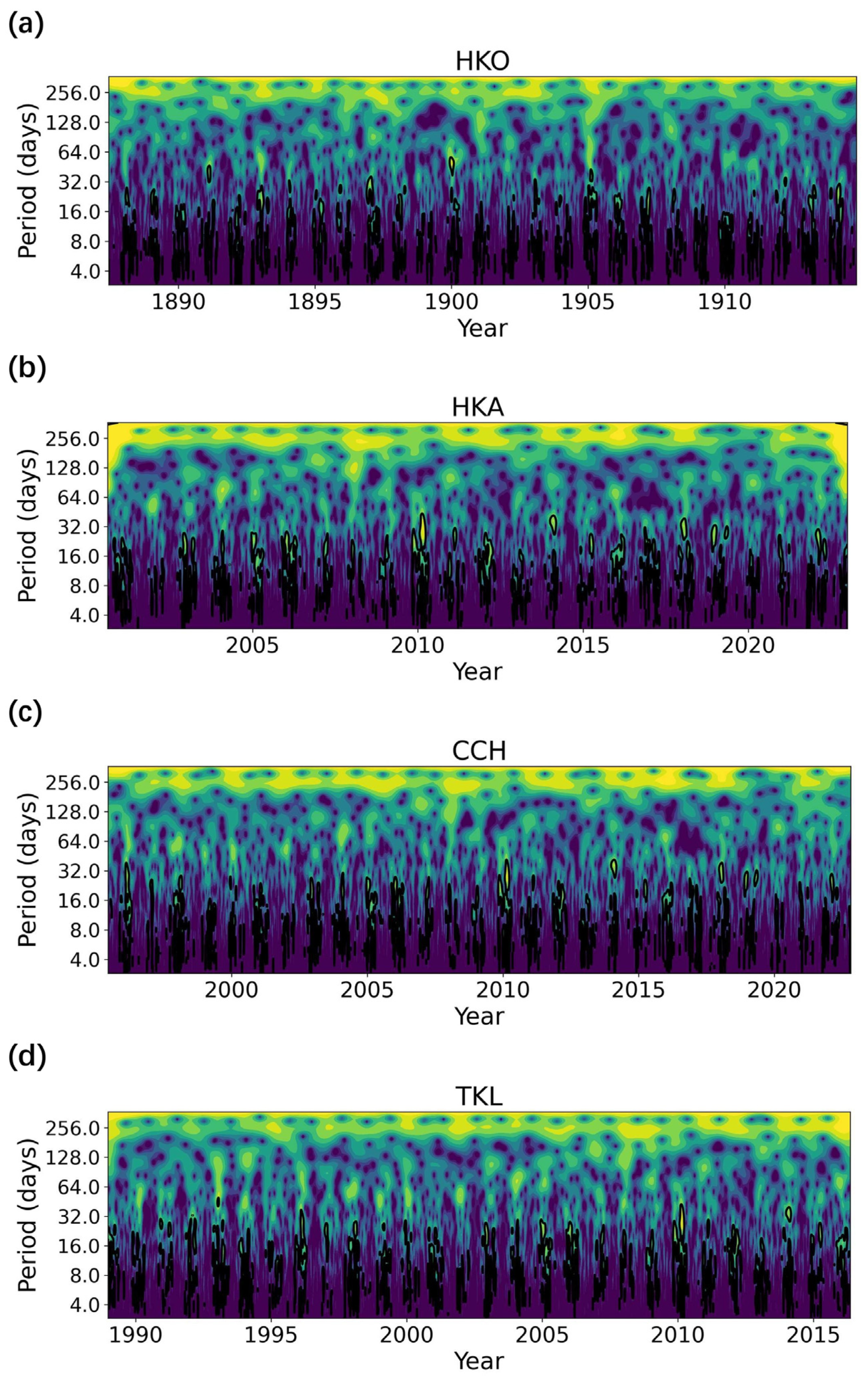
2.2.1. Wavelet Spectral Analysis

In this study, we examine the validity and advantages of the 1D-CNN filter by applying it to extract QBWO and ISO signals from the HKO observation station as an example. Thus, before applying the filter, a wavelet spectral analysis [38,39] is applied to identify the dominant periods of the QBWO and ISO signals in our input data, i.e., daily mean and maximum and minimum surface air temperatures.
Figure 1 presents the wavelet power spectra of the daily average temperatures at the HKO, HKA, CCH, and TKL stations. It is evident that most QBWO and ISO signals stay shorter than 25 days, while some individual events are featured with longer periodic signals of up to 60 days. On this basis, we determine that the primary periods of the QBWO and ISO signals in Hong Kong range from 10 to 60 days.

2.2.2. Lanczos Filter

The Lanczos filter consists of a weight function, which is a combination of the sinc function and the Lanczos window function (a simple sinusoidal shape function). The following is the weight function of the Lanczos filter [42]:
ω k = sin ( 2 π f c k ) π k   ·   sin ( π k / N ) π k / N
where f c represents the cutoff frequency, k is the weight index, and N is the size of the filter’s half-window width, which represents the number of weights on one side of the filter window, that is, the distance from the center point to one side of the window (excluding the center point itself). The total number of weights is 2 N + 1 , including the center point and N weights on both sides. The first term in Equation (1), sin ( 2 π f c k ) π k , is used to extract signals from specific frequencies.
As mentioned in the Section 1, the Lanczos filter is one of the most popular methods used in climate studies. Thus, in this study, the Lanczos filter and its filtering output are considered as the ground truth for training and evaluating the 1D-CNN filter. Specifically, a 121-point Lanczos bandpass filter is applied to the temperature records to extract the QBWO and ISO signals (10–60-day) based on the wavelet spectral analysis results (Figure 1). The filtered outputs are then used for model training and validation in the next step.

2.2.3. Statistical Evaluation and Analysis Methods

In the process of neural network training, this article uses the simple mean square error loss function (MSE) (Equation (2)), which is a common loss function, especially in regression tasks [43]:
M S E = 1 m i = 1 m ( y i f ( x i ) ) 2
where y i and f ( x i ) represent the 1D-CNN filter outputs and the ground truth of the ith sample, respectively, while m denotes the number of samples.
In addition, the root mean square error (RMSE), mean absolute error (MAE) [44], and coefficient of determination ( R 2 ) [45] were also used to evaluate the accuracies of the trained 1D-CNN filter (Equations (3)–(6)). Among them, the RMSE and MAE reflect the differences between the values predicted by 1D-CNN and the values generated by the Lanczos filter. The RMSE is more sensitive to large errors, while the MAE treats all errors equally. R2 represents the goodness of fit of the 1D-CNN.
R M S E =   1 m i = 1 m ( y i f ( x i ) ) 2
M A E = 1 n i = 1 n y i f ( x i )
R 2 = 1 i = 1 n ( y i f ( x i ) ) 2 i = 1 n ( y i f ( x i ) ¯ ) 2  
  f ( x i ) ¯ = 1 n i = 1 n f ( x i )

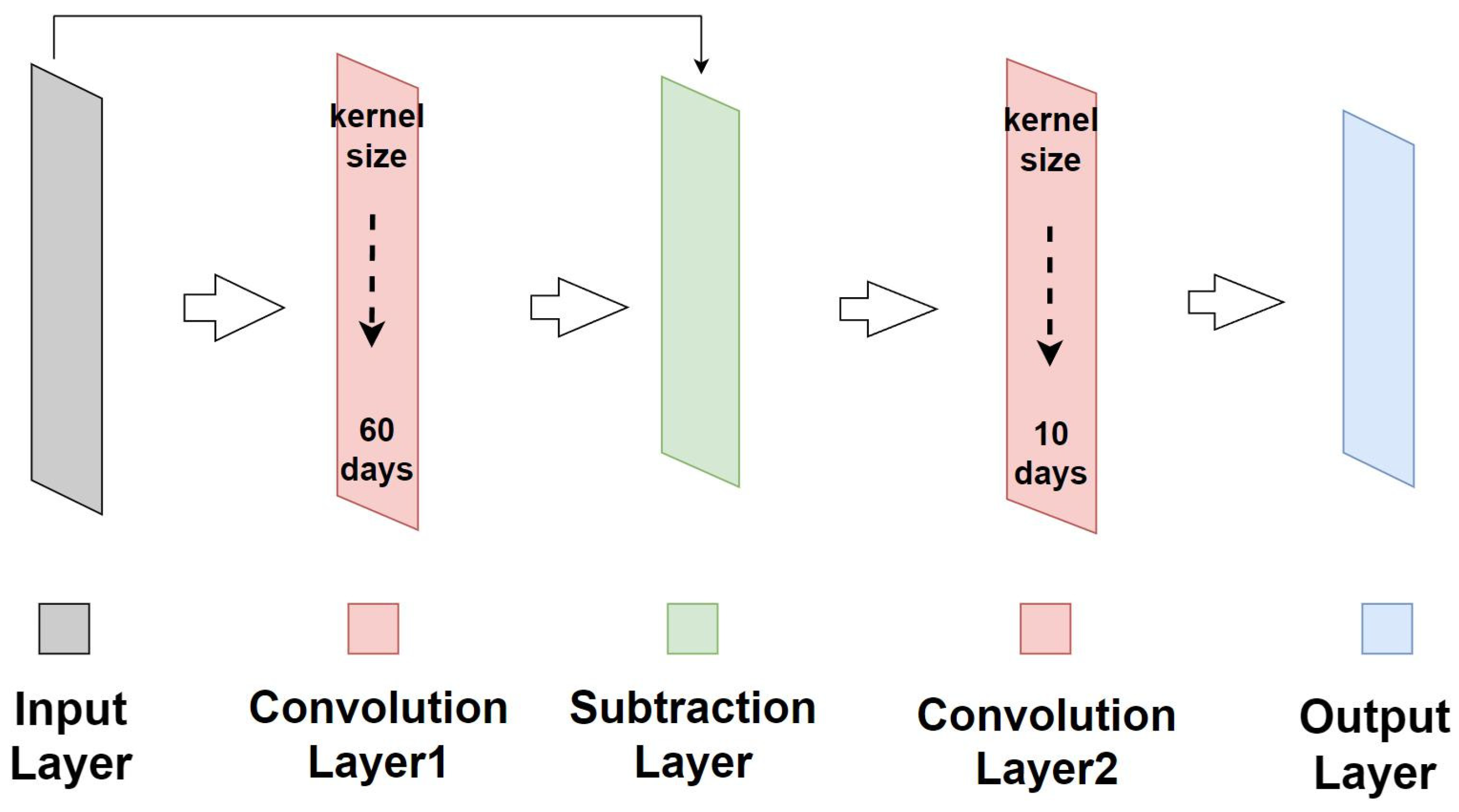
3. Design and Configuration of 1D-CNN Bandpass Filter

Following Stan and Mantripragada [34], the 1D-CNN bandpass filter employed in this study consists of two convolutional layers and one subtraction layer (Figure 2).
Both convolutional layers serve as lowpass filters of different cut-off frequencies or periods, and the subtraction layer is used to remove any unwanted signals. The combination of subtractive and convolutional layers acts as a highpass filter by removing the lowpass-filtered signal generated by the convolutional layer. More specifically, for the 10–60-day 1D-CNN bandpass filter in this study, the first convolutional layer (kernel size = 60 days) is responsible for extracting low-frequency signals with periods exceeding 60 days. Subsequently, a subtraction layer removes these filtered low-frequency signals from the original time series, leaving only variabilities with periods shorter than 60 days. This highpass-filtered signal is then fed into the second convolutional layer (kernel size = 10 days) in order to capture variability within the range of 10 to 60 days. Zero-padding is employed to preserve the data’s dimensions. We can easily convert this 1D-CNN bandpass filter into a highpass filter or a lowpass filter by simply changing the combination of convolutional and subtractive layers.
This article initially divides the input temperature data, which have been processed through a 10–60-day Lanczos filter, into a training set (xtrain), a validation set (xval), and a test set (xtest). The training set includes data from 2006 up to 2019, the validation data are from 2020 to 2021, and the test set consists of data from 2022. Subsequently, a 1D-CNN model is constructed using the PyTorch framework. This model comprises two convolutional layers and one subtraction layer, with the first convolutional layer having a kernel size of 60 and the second convolutional layer having a kernel size of 10. After passing through the first convolutional layer, the output undergoes a subtraction operation—subtracting the output of the first convolutional layer from the original signal—before being forwarded to the second convolutional layer. During the training process, the MSE loss function is employed, and the Adam optimizer is used for parameter optimization. The learning rate is set to 0.001, which determines the step size for parameter updates during the model training process. Epsilon is set to 0.0000001 to avoid division by zero, thereby enhancing the computational stability. The maximum number of training iterations (no_epochs) is set to 10,000, ensuring that the model is adequately trained. In each training epoch, the model performs forward propagation on the training set, computes the loss, and then carries out backpropagation to update the weights. The output data consist of the training set (ytrain), the validation set (yval), and the test set (ytest) after being processed through the 1D CNN filters.

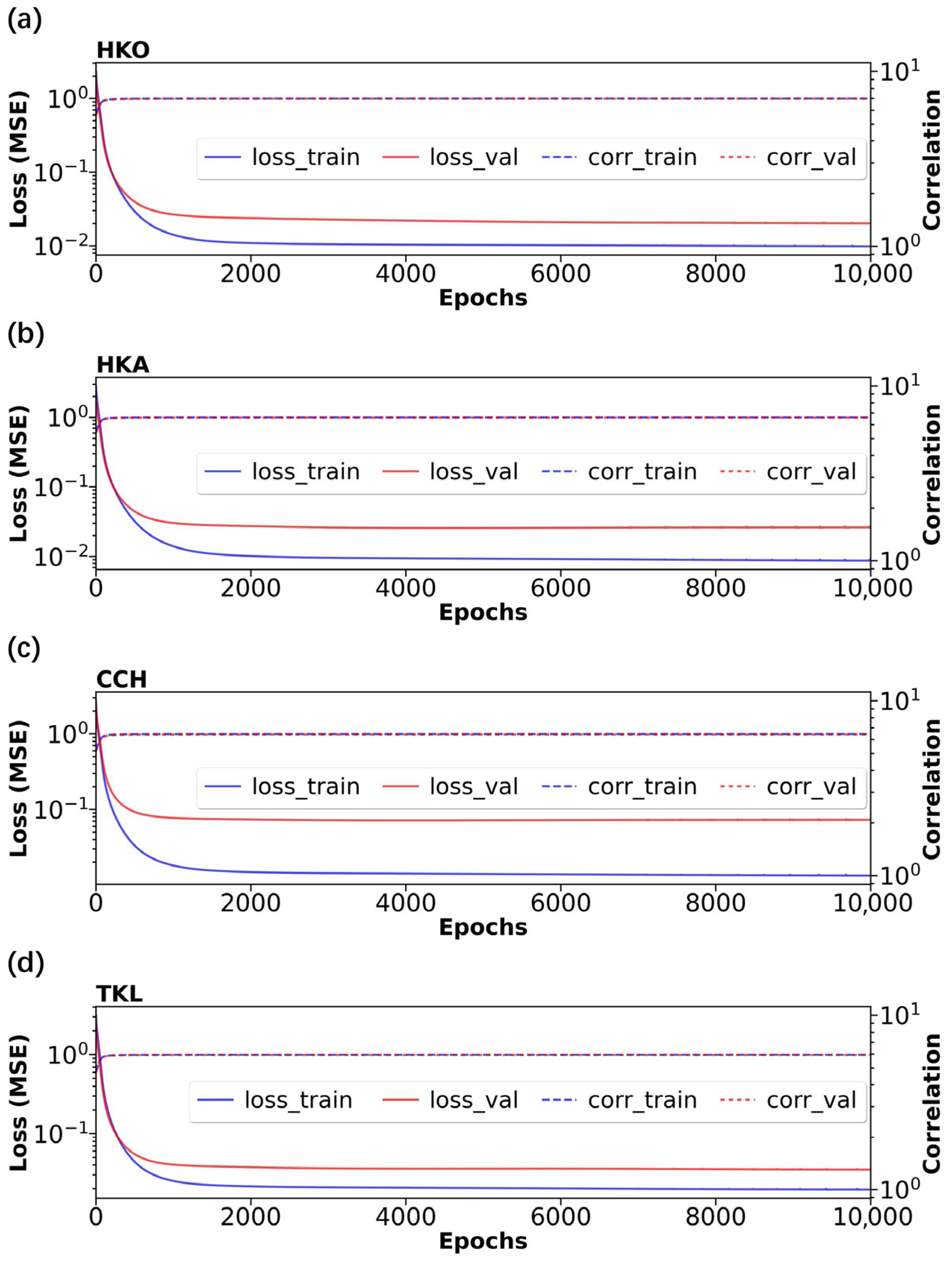
4. Validity of 1D-CNN Bandpass Filter

We first examine the training process of the 1D-CNN filter model. In each training cycle, the losses (MSE) calculated for both training and validation are primarily examined. The correlation coefficient is computed as another metric to verify the performance of the 1D-CNN filter. In the following paragraphs, we take the daily mean temperatures at the HKO, HKA, CCH, and TKL stations as examples to illustrate the validity of the 1D-CNN bandpass filter.
As shown in Figure 3, we find that the model’s loss gradually decreases during the training process and converges to a relatively stable state when the iteration count reaches 2000. The effectiveness of training is evaluated comprehensively through the loss curves and correlation coefficient curves mentioned above. A smaller MSE loss and a higher correlation coefficient indicate that the 1D-CNN filter output is closer to the ground truth, implying better training performance of the 1D-CNN filter. Our results show that for the HKO site, the correlation coefficients between the 1D-CNN and Lanczos filter outputs for the training set and the validation set are approximately 0.9977 and 0.9936, respectively, after 10,000 epochs of training (Figure 3a); for the HKA site, the correlation coefficients for the training set and the validation set are approximately 0.9984 and 0.9933, respectively (Figure 3b); for the CCH site, the correlation coefficients of the training set and the validation set are approximately 0.9970 and 0.9833, respectively (Figure 3c); for the TKL site, the correlation coefficients of the training set and the validation set are approximately 0.9969 and 0.9926, respectively (Figure 3d). The high correlation coefficients between the outputs of the 1D-CNN filter and the Lanczos filter for both the training set and validation set indicate that the 1D-CNN filter can accurately extract QBWO and ISO signals at all of the four stations. This demonstrates that the 1D-CNN filter effectively replicates the results of the Lanczos filter, even though it employs a window length that is half of that of the Lanczos filter.
The validity of the 1D-CNN filtering approach is also evident for all of the other 10 stations employed in this study. We compare the results obtained with the 1D-CNN filter for time series data from the 14 stations between 2010 and 2020 with those obtained using Lanczos filtering. The calculated evaluation metrics, including the MAE, MSE, RMSE, and R2, are presented in Table 2. The MAE values range from 0.053 to 0.066, with a mean value of 0.059. The MSE values range from 0.007 to 0.012, with a mean value of 0.009. The RMSE values range from 0.082 to 0.111, with a mean value of 0.097. The R2 values range from 0.995 to 0.998, with a mean value of 0.996. All these metrics indicate that the 1D-CNN filter is able to reproduce bandpass-filtered signals that are highly consistent with those generated by the Lanczos filter. The evaluation metrics for the 14 stations confirm that the results we obtained are not just cherry-picked examples.
The outstanding performance of the 1D-CNN bandpass filter can be directly illustrated by comparing between the original time series, the time-filtered series processed with a Lanczos filter, and the time-filtered series processed with a 1D-CNN filter. Figure 4 gives a comparison of the HKO, HKA, CCH, and TKL stations in the year 2022. Our results reveal that the time series after 1D-CNN filtering closely matches the time series after Lanczos filtering for the daily average temperatures at all four stations, confirming that the 1D-CNN model has as high of a capability to filter QBWO and ISO signals as the Lanczos filter does. It is also noted that the Lanczos filter may not be able to produce valid filtered outputs when there are missing data points, such as in late April 2022 at the CCH station (Figure 4c). More discussion will be given in the next section on how the 1D-CNN filter could address this issue.

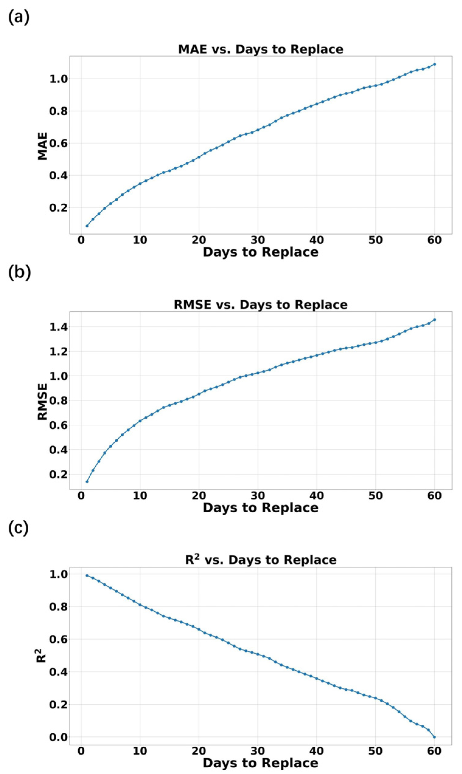
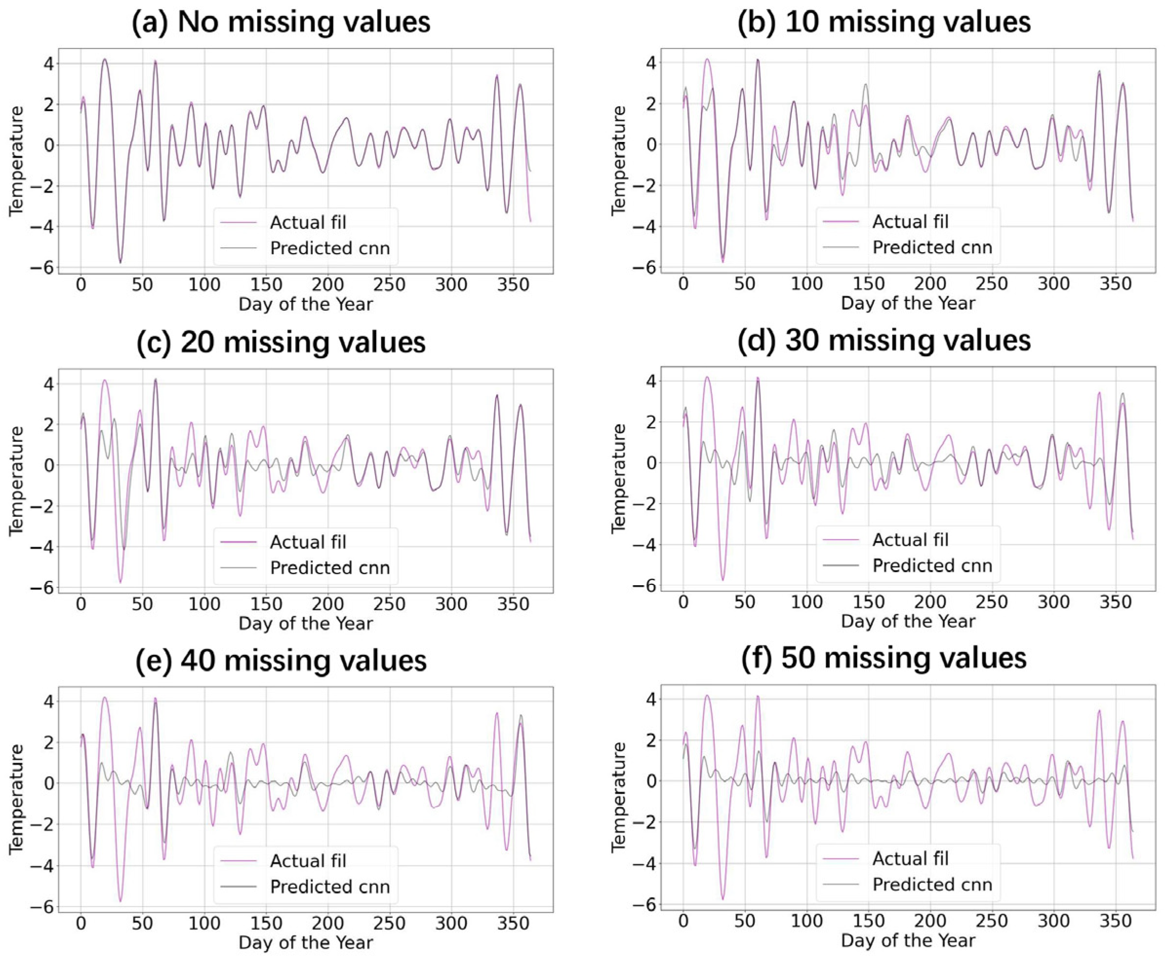
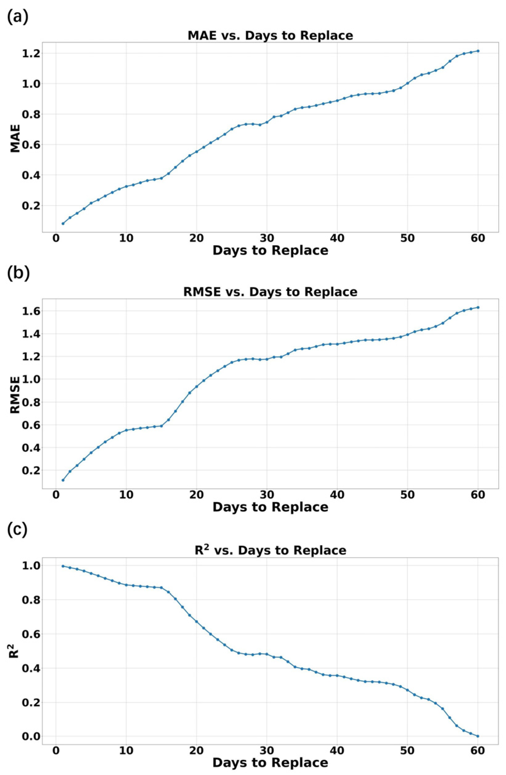
5. Application of 1D-CNN Bandpass Filter to Time Series with Missing Data Points

As mentioned in the Section 1, because the Lanczos filter relies on a certain number of neighboring data points to reduce the artificial oscillations during filtering calculations, this leads to a loss of data at the very beginning and the end of the filtered output, as well as nearby missing values in the input series. Stan and Mantripragada have successfully shown that the 1D-CNN filter is one of the best methods to handle data edges and mitigate this limitation by shortening the length of window [34] without sacrificing the accuracies of filtering calculations, which is also verified in our results in Section 4. However, it remains unclear how well the 1D-CNN filter works with the existence of missing data points in the original input. In this section, a series of tests are carried out to examine the abilities and limitations of the 1D-CNN filter when dealing with time series with missing values.
As with most in situ observations, the daily temperature data of most stations employed in this study do have missing data points due to reasons such as instrument failure, maintenance and replacement, human error, communication failures, outbreak of war, etc. At the positions of the missing points, the leading edge, and the trailing edge, the edge effects of the Lanczos filter can affect the filtering effects in their vicinity. Therefore, a common way is to simply ignore these missing points and return NaN values in the filtering outputs. This causes difficulties for us to examine the accuracies of 1D-CNN filter outputs by taking the Lanczos filter as the ground truth.
To address this problem, we employ the HKO station observations, of which the data remain continuous throughout the period from 1947 to 2022. By applying the 10–60-day Lanczos filter to the HKO daily temperature data in this period, we first obtain the ground truth of the QBWO-to-ISO signals. After that, we manually replace data points in the original time series with missing values according to a predetermined interval (from 1 to 60 days). Subsequently, the pre-trained 1D-CNN bandpass filter, by the procedures introduced in Section 3, is applied to series with manually entered missing data points. Finally, the results between the ground truth (i.e., Lanczos filter output) and the 1D-CNN filter outputs with different numbers of missing values are compared based on the MAE, RMSE, and R2. These procedures give clues about the impact of missing values on 1D-CNN filtering performance. In the following discussion, one missing data point refers to one missing value for every 60 days, two missing data points refer to two missing values for every 60 days, and so on. Comparison is carried out for the period of 2010–2020.
Our results reveal that the 1D-CNN filter still maintains a high level of accuracy even when some data points are missing. However, as the number of missing values increases, the model’s errors generally show a growing trend. Figure 5 clearly shows that as the number of missing values increases, the MAE and RMSE increase rapidly when the number of missing values is fewer than 10, and the increasing trend remains rather steady after that. R2 exhibits similar patterns, but with opposite signs in the trend because of its inversely proportional relationship with error. This shows that as the number of missing values increases, the accuracy of the 1D-CNN filter gradually becomes lower. The above results indicate that the 1D-CNN filter is able to withstand a limited number of missing data points.
What is the largest number of missing data points that the 1D-CNN filter can withstand? In this study, we set R2 ≥ 0.8 as the minimum accuracy criterion for an acceptable 1D-CNN filter, which indicates that the filtering output explains more than 80% of the ground truth-filtered signals. According to Figure 5c, R2 drops from 0.991 for 1 missing data point to 0.811 for 10 missing data points. Therefore, based on this criterion, we conclude that the 1D-CNN filter can allow up to 10 days of missing values, which accounts for 16.67% of the length of filter window (i.e., 60 days, or the kernel size of the first convolutional layer).
As an example, Figure 6 compares the time series of the filtered daily average temperature with the ground truth at the HKO site in 2018. Panels (a) to (f) present results with difference numbers of missing data points. The results show that the 1D-CNN filtering results are entirely consistent with the Lanczos filtering output when there are no missing data points (Figure 6a). When the number of data points is set to 10, while the 1D-CNN filter can capture most of the QBWO and ISO variability, it starts to produce some errors, such as slightly overestimating or underestimating some of the peaks and troughs (Figure 6b). In this case, the MAE, RMSE, and R2 are 0.325, 0.554, and 0.885, respectively (Figure 7). As the number of missing data points increases to 20, the inconsistencies between the two series become larger (Figure 6c) and R2 drops to 0.672. Based on the R2 ≥ 0.8 criterion, the 1D-CNN-filtered series shown in Figure 6c is considered to have failed to accurately capture the overall 10–60-day signals. The same is also observed for 30, 40, and 50 missing data points (Figure 6d–f).

6. Conclusions and Discussion

This study aims to address the limitations of traditional temporal filters in extracting certain signals from discontinuous time series, which are commonly seen in meteorological and climate research. Making use of machine learning techniques, we applied a 1D-CNN temporal filter to daily temperature observations from the Hong Kong Observatory, examined its validity, and explored its ability to filter time series with missing data points. The key contributions of this paper are as follows:
(1)
A 1D-CNN temporal filter, which can be transformed into a highpass, bandpass, or lowpass filter, is developed.
(2)
The 1D-CNN filter is shown to be good at handling discontinuous time series.
(3)
The 1D-CNN filter allows a maximum number of missing data points that is approximately 16.67% of the filter window length. In other words, say, for a 100-day lowpass filter, the 1D-CNN filter is able to give relatively accurate filtered results even if there are ~17 missing values within a 100-day window.
It is important to note here that the 1D-CNN bandpass filter presented in this study can be extended to other types of temporal filters, such as highpass and lowpass filters. Namely, a lowpass filter only requires one convolutional layer; a highpass one requires an additional subtraction layer after the convolutional layer; and a bandpass filter can be constructed by combining a highpass and a lowpass filter, as explained in Section 3. The corresponding code, written in Pytorch, is publicly available at (https://github.com/jeremychleung/1DCNN_Filter, accessed on 2 May 2024). The validity of the 1D-CNN temporal filter has been verified in Section 4 and also by Stan and Mantripragada [34]. However, the ability of 1D-CNN highpass and lowpass filters to handle missing input data points was not explicitly discussed in this paper and needs further analyses.
Another important remark is that the maximum number of missing data points allowed depends on various factors, such as variables, data types, regions, period, etc. Although our analyses revealed that the presented 1D-CNN bandpass filter allows a maximum number of missing data points of 16.67% of the filter window length, this conclusion may not be applicable to different application scenarios. It is recommended to re-examine the limits of the 1D-CNN filter beforehand.
To conclude, this study demonstrates that the 1D-CNN filter can effectively address the limitations of Lanczos and other filters when handling time series with missing data points. Although the discussion of this paper is focused on bandpass filtering, the findings also hold for highpass and lowpass filters. This finding provides an alternative way to extract atmospheric variability signals from certain time scales, especially when traditional filters fail to work well for discontinuous time series. The introduced 1D-CNN filter will be particularly useful in signal extractions from datasets that contain missing values and also in real-time operational applications, such as S2S monitoring and forecasting and the filtering of numerical instability [46]. By exploring this innovative approach, this study also demonstrates another potential for applying machine learning algorithms in this field of research.

Author Contributions

Conceptualization, H.K. and J.C.-H.L.; methodology, H.K. and J.C.-H.L.; software, D.Y.; validation, D.Y., H.K. and J.C.-H.L.; formal analysis, D.Y., H.K. and J.C.-H.L.; investigation, D.Y., H.K. and J.C.-H.L.; resources, P.W.C.; data curation, P.W.C.; writing—original draft preparation, D.Y., H.K. and J.C.-H.L.; writing—review and editing, D.Y., H.K., J.C.-H.L., P.W.C., C.F., Y.W. and B.Z.; visualization, D.Y.; supervision, H.K., J.C.-H.L. and P.W.C.; project administration, H.K. and J.C.-H.L.; funding acquisition, Y.W. and B.Z. All authors have read and agreed to the published version of the manuscript.

Funding

This work is funded and supported by the Japan Society for the Promotion of Science (KAKENHI 24K01140), the Great Britain Sasakawa Foundation (J863), the Guangdong Basic and Applied Basic Research Foundation (2020A1515110275), the Guangdong Province Introduction of Innovative R&D Team Project (2019ZT08G669).

Institutional Review Board Statement

Not applicable.

Informed Consent Statement

Not applicable.

Data Availability Statement

The station observation data analyzed in this paper were provided by the Hong Kong Observatory. Data are available on reasonable request from the authors. The codes for constructing the 1D-CNN filter in this study is publicly available at (https://github.com/jeremychleung/1DCNN_Filter, accessed on 2 May 2024). Other codes used for analyses in this study are available on reasonable request from the authors (chleung@pku.edu.cn or konghoiio@pku.edu.cn).

Conflicts of Interest

The authors declare no conflicts of interest.

References

  1. Wang, B.; Ding, Y.; Sikka, D. Synoptic systems and weather. In The Asian Monsoon; Springer: Berlin/Heidelberg, Germany, 2006; pp. 131–201. [Google Scholar]
  2. Sheridan, S.C.; Lee, C.C. Synoptic climatology and the general circulation model. Prog. Phys. Geogr. 2010, 34, 101–109. [Google Scholar] [CrossRef]
  3. Qian, W.; Leung, J.C.-H.; Ren, J.; Du, J.; Feng, Y.; Zhang, B. Anomaly based synoptic analysis and model prediction of six dust storms moving from Mongolia to northern China in spring 2021. J. Geophys. Res. Atmos. 2022, 127, e2021JD036272. [Google Scholar] [CrossRef]
  4. Loikith, P.C.; Pampuch, L.A.; Slinskey, E.; Detzer, J.; Mechoso, C.R.; Barkhordarian, A. A climatology of daily synoptic circulation patterns and associated surface meteorology over southern South America. Clim. Dyn. 2019, 53, 4019–4035. [Google Scholar] [CrossRef]
  5. Wang, J.; Guan, Y.; Wu, L.; Guan, X.; Cai, W.; Huang, J.; Dong, W.; Zhang, B. Changing lengths of the four seasons by global warming. Geophys. Res. Lett. 2021, 48, e2020GL091753. [Google Scholar] [CrossRef]
  6. Gan, Q.; Leung, J.C.-H.; Wang, L.; Zhang, B. Weakening seasonality of Indo-Pacific warm pool size in a warming world since 1950. Environ. Res. Lett. 2023, 18, 014024. [Google Scholar] [CrossRef]
  7. Santer, B.D.; Po-Chedley, S.; Zelinka, M.D.; Cvijanovic, I.; Bonfils, C.; Durack, P.J.; Fu, Q.; Kiehl, J.; Mears, C.; Painter, J.; et al. Human influence on the seasonal cycle of tropospheric temperature. Science 2018, 361, eaas8806. [Google Scholar] [CrossRef] [PubMed]
  8. Longandjo, G.-N.T.; Rouault, M. Revisiting the Seasonal Cycle of Rainfall over Central Africa. J. Clim. 2024, 37, 1015–1032. [Google Scholar] [CrossRef]
  9. Cai, W.; Santoso, A.; Collins, M.; Dewitte, B.; Karamperidou, C.; Kug, J.S.; Lengaigne, M.; McPhaden, M.J.; Stuecker, M.F.; Taschetto, A.S.; et al. Changing El Niño–Southern oscillation in a warming climate. Nat. Rev. Earth Environ. 2021, 2, 628–644. [Google Scholar] [CrossRef]
  10. Lin, J.; Qian, T. A new picture of the global impacts of El Nino-Southern oscillation. Sci. Rep. 2019, 9, 17543. [Google Scholar] [CrossRef]
  11. Cai, W.; Santoso, A.; Wang, G.; Yeh, S.-W.; An, S.-I.; Cobb, K.M.; Collins, M.; Guilyardi, E.; Jin, F.-F.; Kug, J.-S.; et al. ENSO and greenhouse warming. Nat. Clim. Chang. 2015, 5, 849–859. [Google Scholar] [CrossRef]
  12. Haines, A.; Lam, H.C. El Niño and health in an era of unprecedented climate change. Lancet 2023, 402, 1811–1813. [Google Scholar] [CrossRef] [PubMed]
  13. Zhang, C. Madden–Julian oscillation: Bridging weather and climate. Bull. Am. Meteorol. Soc. 2013, 94, 1849–1870. [Google Scholar] [CrossRef]
  14. Liu, F.; Wang, B.; Ouyang, Y.; Wang, H.; Qiao, S.; Chen, G.; Dong, W. Intraseasonal variability of global land monsoon precipitation and its recent trend. NPJ Clim. Atmos. Sci. 2022, 5, 30. [Google Scholar] [CrossRef]
  15. Leung, J.C.-H.; Qian, W. Monitoring the Madden–Julian oscillation with geopotential height. Clim. Dyn. 2017, 49, 1981–2006. [Google Scholar] [CrossRef]
  16. Zhang, C. Madden-julian oscillation. Rev. Geophys. 2005, 43, RG2003. [Google Scholar] [CrossRef]
  17. Tanaka, H.L.; Ishizaki, N.; Kitoh, A. Trend and interannual variability of Walker, monsoon and Hadley circulations defined by velocity potential in the upper troposphere. Tellus A Dyn. Meteorol. Oceanogr. 2004, 56, 250–269. [Google Scholar] [CrossRef]
  18. Gan, Q.; Wang, L.; Leung, J.C.H.; Weng, J.; Zhang, B. Recent weakening relationship between the springtime Indo-Pacific warm pool SST zonal gradient and the subsequent summertime western Pacific subtropical high. Int. J. Climatol. 2022, 42, 10173–10194. [Google Scholar] [CrossRef]
  19. Crhová, L.; Holtanová, E. Temperature and precipitation variability in regional climate models and driving global climate models: Total variance and its temporal-scale components. Int. J. Climatol. 2019, 39, 1276–1286. [Google Scholar] [CrossRef]
  20. Liang, M.C.; Li, K.F.; Shia, R.L.; Yung, Y.L. Short-period solar cycle signals in the ionosphere observed by FORMOSAT-3/COSMIC. Geophys. Res. Lett. 2008, 35, L15818. [Google Scholar] [CrossRef]
  21. Russell, D.R. Development of a time-domain, variable-period surface-wave magnitude measurement procedure for application at regional and teleseismic distances, part I: Theory. Bull. Seismol. Soc. Am. 2006, 96, 665–677. [Google Scholar] [CrossRef]
  22. Duchon, C.E. Lanczos filtering in one and two dimensions. J. Appl. Meteorol. Climatol. 1979, 18, 1016–1022. [Google Scholar] [CrossRef]
  23. Zhang, J.; Wang, H.; Liu, F. Inter-annual variability of boreal summer intra-seasonal oscillation propagation from the Indian ocean to the Western Pacific. Atmosphere 2019, 10, 596. [Google Scholar] [CrossRef]
  24. Ajayamohan, R.; Rao, S.A.; Luo, J.J.; Yamagata, T. Influence of Indian Ocean Dipole on boreal summer intraseasonal oscillations in a coupled general circulation model. J. Geophys. Res. Atmos. 2009, 114, D06119. [Google Scholar] [CrossRef]
  25. Arguez, A.; Bourassa, M.A.; O’Brien, J.J. Detection of the MJO signal from QuikSCAT. J. Atmos. Ocean. Technol. 2005, 22, 1885–1894. [Google Scholar] [CrossRef]
  26. Leung, J.C.-H.; Qian, W.; Zhang, P.; Zhang, B. Geopotential-based Multivariate MJO Index: Extending RMM-like indices to pre-satellite era. Clim. Dyn. 2022, 59, 609–631. [Google Scholar] [CrossRef]
  27. Roman-Stork, H.L.; Subrahmanyam, B.; Murty, V. Quasi-biweekly oscillations in the Bay of Bengal in observations and model simulations. Deep Sea Res. Part II Top. Stud. Oceanogr. 2019, 168, 104609. [Google Scholar] [CrossRef]
  28. Wei, W.; Zhang, R.; Yang, S.; Li, W.; Wen, M. Quasi-biweekly oscillation of the South Asian high and its role in connecting the Indian and East Asian summer rainfalls. Geophys. Res. Lett. 2019, 46, 14742–14750. [Google Scholar] [CrossRef]
  29. Tong, Q.; Yao, S. The quasi-biweekly oscillation of winter precipitation associated with enso over southern China. Atmosphere 2018, 9, 406. [Google Scholar] [CrossRef]
  30. Zhang, Y.; Li, T.; Gao, J.; Wang, W. Origins of quasi-biweekly and intraseasonal oscillations over the South China Sea and Bay of Bengal and scale selection of unstable equatorial and off-equatorial modes. J. Meteorol. Res. 2020, 34, 137–149. [Google Scholar] [CrossRef]
  31. Yan, X.; Yang, S.; Wang, T.; Maloney, E.D.; Dong, S.; Wei, W.; He, S. Quasi-biweekly oscillation of the Asian monsoon rainfall in late summer and autumn: Different types of structure and propagation. Clim. Dyn. 2019, 53, 6611–6628. [Google Scholar] [CrossRef]
  32. Sultan, B.; Janicot, S. Abrupt shift of the ITCZ over West Africa and intra-seasonal variability. Geophys. Res. Lett. 2000, 27, 3353–3356. [Google Scholar] [CrossRef]
  33. McNeall, D.; Halloran, P.R.; Good, P.; Betts, R.A. Analyzing abrupt and nonlinear climate changes and their impacts. Wiley Interdiscip. Rev. Clim. Chang. 2011, 2, 663–686. [Google Scholar] [CrossRef]
  34. Stan, C.; Mantripragada, R.S.S. A deep learning filter for the intraseasonal variability of the tropics. Artif. Intell. Earth Syst. 2023, 2, e220079. [Google Scholar] [CrossRef]
  35. Haidar, A.; Verma, B. Monthly rainfall forecasting using one-dimensional deep convolutional neural network. IEEE Access 2018, 6, 69053–69063. [Google Scholar] [CrossRef]
  36. Sari, Y.R.; Djamal, E.C.; Nugraha, F. Daily rainfall prediction using one dimensional convolutional neural networks. In Proceedings of the 2020 3rd International Conference on Computer and Informatics Engineering (IC2IE), Yogyakarta, Indonesia, 15–16 September 2020; IEEE: Piscataway, NJ, USA, 2020; pp. 90–95. [Google Scholar]
  37. Chen, W.; Ho, C.-H.; Yang, S.; Wu, Z.; Chen, H. Modulations of Madden–Julian Oscillation and Quasi-Biweekly Oscillation on Early Summer Tropical Cyclone Genesis over the Bay of Bengal and South China Sea. J. Clim. 2024, 37, 1951–1964. [Google Scholar] [CrossRef]
  38. Ge, Z. Significance tests for the wavelet power and the wavelet power spectrum. Ann. Geophys. 2007, 25, 2259–2269. [Google Scholar] [CrossRef]
  39. Chen, G.; Sui, C.H. Characteristics and origin of quasi-biweekly oscillation over the western North Pacific during boreal summer. J. Geophys. Res. Atmos. 2010, 115, D14113. [Google Scholar] [CrossRef]
  40. Allen, M.R.; Smith, L.A. Investigating the origins and significance of low-frequency modes of climate variability. Geophys. Res. Lett. 1994, 21, 883–886. [Google Scholar] [CrossRef]
  41. Gilman, D.L.; Fuglister, F.J.; Mitchell, J.M. On the power spectrum of “red noise”. J. Atmos. Sci. 1963, 20, 182–184. [Google Scholar] [CrossRef]
  42. Taquet, J.; Labit, C. Optimized decomposition basis using Lanczos filters for lossless compression of biomedical images. In Proceedings of the 2010 IEEE International Workshop on Multimedia Signal Processing, Saint-Malo, France, 4–6 October 2010; IEEE: Piscataway, NJ, USA, 2010; pp. 122–127. [Google Scholar]
  43. Marmolin, H. Subjective MSE measures. IEEE Trans. Syst. Man Cybern. 1986, 16, 486–489. [Google Scholar] [CrossRef]
  44. Willmott, C.J.; Matsuura, K. Advantages of the mean absolute error (MAE) over the root mean square error (RMSE) in assessing average model performance. Clim. Res. 2005, 30, 79–82. [Google Scholar] [CrossRef]
  45. Ozer, D.J. Correlation and the coefficient of determination. Psychol. Bull. 1985, 97, 307. [Google Scholar] [CrossRef]
  46. Haltiner, G.J. Numerical Weather Prediction; John Wiley and Sons: New York, NY, USA, 1971; 317p. [Google Scholar]
Figure 1. The wavelet energy spectra of daily average temperatures at the (a) HKO, (b) HKA, (c) CCH, and (d) TKL stations. Black contours denote results that are statistically significant at the 95% confidence level for the red noise-based significance test. The significance test was performed under the red noise assumption because time series of meteorological variables are mostly serially correlated in time, in which background noise does not obey the white noise assumption [40,41].
Applsci 14 06289 g001
Figure 2. Model structure diagram of one-dimensional convolutional neural network.
Applsci 14 06289 g002
Figure 3. The MSE losses (unit: °C; solid lines) and correlation coefficients (dashed lines) between the outputs of 1D-CNN filter and Lanczos filter during the training process (blue) and validation process (red). Results are based on the daily mean temperature observations of the (a) HKO, (b) HKA, (c) CCH, and (d) TKL stations.
Applsci 14 06289 g003
Figure 4. Time series of the original input data (blue solid line), daily climatology (blue dashed line), unfiltered daily anomaly (red solid line), Lanczos-filtered output (purple solid line), and 1D-CNN-filtered output (black solid line) from January to December 2022. Results are based on the daily mean temperature observations of the (a) HKO, (b) HKA, (c) CCH, and (d) TKL stations.
Applsci 14 06289 g004
Figure 5. Changes in (a) MAE, (b) RMSE, and (c) R2 of the 1D-CNN filtering results against the number of missing values at the HKO station from 2010 to 2020.
Applsci 14 06289 g005
Figure 6. Time series of Lanczos-filtered series (purple line) and 1D-CNN-filtered series (black line) of daily average temperatures at the HKO site in 2018. The 1D-CNN-filtered results are obtained based on (a) no missing values and (b) 10, (c) 20, (d) 30, (e) 40, and (f) 50 missing data points.
Applsci 14 06289 g006
Figure 7. Changes in (a) MAE, (b) RMSE, and (c) R2 of the 1D-CNN filtering results against the number of missing values at the HKO station in 2018.
Applsci 14 06289 g007
Table 1. Information about 14 automatic weather stations employed in this study. Note that all weather stations are still operating in present day.
Automatic
Weather
Station
PositionLength of Data RecordNumber of Missing Values
Latitude
N
Longitude
E
Starting
Date
Number of
Data Points
Mean
Temperature
Max/Min
Temperature
Ta Kwu Ling
(TKL)
22°
31′43″
114°
09′24″
14 October 198513,59310911043
Lau Fau Shan (LFS)22°
28′08″
113°
59′01″
16 September 198513,621222147
Wetland Park (WLP)22°
28′00″
114°
00′32″
10 November 20056261137
Shek Kong (SEK)22°
26′10″
114°
05′05″
4 November 19969554342293
Tai Mo Shan (TMS)22°
24′38″
114°
07′28″
1 December 19969527231179
Sha Tin
(SHA)
22°
24′09″
114°
12′36″
1 October 198413,971154111
Tate’s Cairn (TC)22°
21′28″
114°
13′04″
1 December 1997916210666
King’s Park (KP)22°
18′43″
114°
10′22″
1 July 199211,141257
Hong Kong International Airport (HKA)22°
18′34″
113°
55′19″
1 June 19979345031
Hong Kong Observatory (HKO)22°
18′07″
114°
10′27″
1 April 188450,67825572557
Sha Lo Wan (SLW)22°
17′28″
113°
54′25″
25 February 199310,902691591
Peng Chau (PEN)22°
17′28″
114°
02′36″
1 June 200467885332
Cheung Chau (CCH)22°
12′04″
114°
01′36″
30 March 199211,2349844
Waglan Island (WGL)22°
10′56″
114°
18′12″
22 August 198912,185811665
Table 2. List of MAE, MSE, RMSE, and R2 values for the test set of all 14 stations from 2010 to 2020.
Automatic
Weather Station
MAEMSERMSER2
Ta Kwu Ling (TKL)0.0660.0120.1110.996
Lau Fau Shan (LFS)0.0630.0120.1080.996
Wetland Park (WLP)0.0610.0100.1010.996
Shek Kong (SEK)0.0640.0110.1040.997
Tai Mo Shan (TMS)0.0590.0120.1070.995
Sha Tin (SHA)0.0580.0080.0920.997
Tate’s Cairn (TC)0.0620.0110.1040.996
King’s Park (KP)0.0550.0090.0930.996
Hong Kong International Airport (HKA)0.0570.0090.0940.997
Hong Kong Observatory (HKO)0.0530.0070.0850.997
Sha Lo Wan (SLW)0.0600.0070.0820.998
Peng Chau (PEN)0.0550.0080.0910.996
Cheung Chau (CCH)0.0550.0080.0910.996
Waglan Island (WGL)0.0530.0080.0920.995
Disclaimer/Publisher’s Note: The statements, opinions and data contained in all publications are solely those of the individual author(s) and contributor(s) and not of MDPI and/or the editor(s). MDPI and/or the editor(s) disclaim responsibility for any injury to people or property resulting from any ideas, methods, instructions or products referred to in the content.

