Longitudinal Nonlinear Equivalent Continuous Model for Shield Tunnel under Coupling of Longitudinal Axial Force and Bending Moment

Abstract

The longitudinal equivalent continuous model generally only studies the stiffness of shield tunnels under longitudinal bending moments, considering it a constant. However, in actual engineering, shield tunnels are exposed to complex environments where seismic events, uneven settlement, etc., may cause simultaneous axial forces and bending moments between segmental rings, necessitating consideration of the longitudinal stiffness of shield tunnels under coupled axial force and bending moment effects. Therefore, based on the influence of different axial forces and bending moments on the separation effect between segmental rings, this study establishes a longitudinal nonlinear equivalent continuous model. Using Guangzhou Metro Line 18 as a case study background, a numerical model of segment ring-bolt is established for comparative analysis. The results show that the contact states between segmental rings can be classified into three modes: completely separated, completely in contact, and partially in contact. Longitudinal bending stiffness remains constant in modes 1 and 2 but decreases with decreasing e in mode 3. The numerically simulated $\phi -e$ curves are consistent with the theoretical results. At the special point $e_0$, the numerical simulation result is −57.27° compared to the theoretical result of −59.66°; at point $e_{\phi 0}$ (−0.3036), the numerical simulation result is close to 0°. The longitudinal bending stiffness curve shows an overall decreasing trend. When $e\le -{\displaystyle \frac{2}{r}}$, which corresponds to mode 2, the longitudinal bending stiffness remains constant at $\pi r^3{E}_{c}t$. As the longitudinal axial pressure decreases, the longitudinal bending stiffness continues to decrease when $-{\displaystyle \frac{2}{r}}\le e\le e_{\phi 0}$. When the longitudinal axial pressure decreases to 0, then the tensile force gradually increases ($e_{\phi 0}\le e\le {\displaystyle \frac{2}{r}}$). $-{\displaystyle \frac{2}{r}}\le e\le {\displaystyle \frac{2}{r}}$ belongs to mode 3, and the equivalent bending stiffness is ${\displaystyle \frac{2(1+sin\phi )r^3{E}_{c}t}{{A_4^{\prime }-A}_3^{\prime }er}}$. As tension continues to increase, when $e\ge {\displaystyle \frac{2}{r}}$, the stiffness no longer decreases, and the longitudinal bending stiffness is ${\displaystyle \frac{\pi r^3{E}_{c}t}{u+1}}$, which belongs to mode 1. The overall trend of the tensile and compressive stiffness curves is an inverse proportional function, with the middle mutation point at $\phi =0$, i.e., $e_{\phi 0}={\displaystyle \frac{-4u}{(2+u)\pi r}}\approx -0.3036$. The findings of this study can provide a basis for the rational calculation of longitudinal forces in shield tunnels in engineering applications.

1. Introduction

Shield tunnels are assembled structures consisting of concrete segments and connecting bolts that exhibit discontinuities in both the transverse (ring) and longitudinal directions [1,2]. Generally speaking, for the study of shield tunnel transverse direction, the problem can be simplified to plane strain when the joints in each segmental ring are limited and the stress characteristics of the shield tunnel are relatively clear [3,4,5]. In contrast, the large longitudinal scale of the shield tunnel, the complex working conditions of the traversing strata, and the large number of circumferential joints between the rings make the longitudinal stress and deformation of the shield tunnel very complicated.

For the longitudinal deformation analysis of shield tunnels, the most applied model is the longitudinal equivalent continuous model (LECM) proposed by Yukio Shibo [6]. The model considers the longitudinal tension, bending, and compression of the shield tunnel independently and gives the solution method for its deformation stiffness, respectively. Guo et al. [7] investigated the longitudinal earthquake response characteristics of the shield tunnels subjected to single-degree-of-freedom seismic excitation and pointed out that when the seismic load is excited horizontally, horizontal bending mainly occurs in shield tunnels, and longitudinal tensile and compressive compression mainly occur in shield tunnels when the seismic load is excited longitudinally. Similarly, based on the LECM, Zhang et al. [8] carried out a series of model tests to investigate the seismic response characteristics of shield tunnels across soft and hard, uneven strata. Wang et al. [9] conducted centrifuge shaking-table tests by considering the shield tunnel as a continuous structure in the longitudinal direction. The above results indicate that LECM has certain engineering applicability, and the calculations are relatively simple. However, when shield tunnels deform under complex external loads, the accuracy of tunnel internal forces calculated using LECM may decrease.

In order to better clarify the longitudinal deformation characteristics of shield tunnels, many experts conduct research using numerical simulation or model tests. The longitudinal deformation characteristics of shield tunnels could be visualized and clarified by discretizing the segments and bolts using the above methods. Li et al. [10] prepared a discrete model to investigate the longitudinal bending stiffness of shield tunnels under varying axial forces. Dong et al. [11] investigated the longitudinal seismic performance of shield tunnels using incremental dynamic analysis and the spring-beam model. Lu et al. [12] used the Shantouwan shield tunnel as the background to establish a 3D fine finite element model to research the damping behavior of shape memory alloy (SMA) flexible joints under seismic loading. Zhang et al. [13] established a 3D finite element model of segment-bolt joints and investigated the seismic deformation characteristics of different types of bolt joints, and the results showed that the stress in the oblique bolt is the maximum, whereas the stress in the curved bolt is the minimum. Zhang et al. [14] established a refined numerical model of the anchor joint and investigated the tension and stress distribution characteristics of the joint under different directions of earthquake. Zhang et al. [15] used cement mortar to prepare the joints, simulated bolts with steel wire, and conducted shaking table tests under soft soil conditions to investigate the seismic response differences of shield tunnels to near-field and far-field ground motion. Zhang et al. [16] investigated the earthquake response characteristics of tunnel-shaft junctions under longitudinal earthquake excitation by using discrete segmental splicing. Guo et al. [17] investigated the influence of the internal structure of the shield tunnel on its longitudinal stiffness by model test and pointed out that the longitudinal stiffness of the tunnel structure is significantly improved when the internal structure is considered. Liu et al. [18] introduced the concrete parameters into numerical simulation and investigated the influence of the nonlinear damage characteristics of concrete materials on the longitudinal deformation characteristics of shield tunnels. Model tests or numerical simulations can intuitively observe the longitudinal deformation characteristics of shield tunnels, but they involve higher operating costs and have certain limitations in engineering analysis.

Building upon the results of numerical simulations and model tests, many researchers have conducted theoretical studies to establish a longitudinal analytical model for shield tunnels. Wu et al. [19] proposed a tunnel-soil interaction model based on the Timoshenko beam simplified model for a tunnel on an elastic foundation, which could consider the shearing dislocation in circumferential joints. Cheng et al. [20] present a simplified method to evaluate the longitudinal behavior of shield tunnels adjacent to braced excavations. An appropriate model was adopted to study both shear and bending deformation of segmental rings, based on the Timoshenko beam theory. Liu et al. [21] proposed a numerical model using homogeneous solid segmental ring-spring elements to understand the longitudinal structural deformation mechanism of shield tunnel linings, which includes a novel treatment for circumferential joints validated with field data. Huang et al. [22] introduced an analytical solution for the longitudinal response of shield tunnel linings, explicitly considering ring-to-ring interactions via two-directional joint springs and employing the state space method. Zhang et al. [23] demonstrated the inherent nonlinearity of segmental joints through analytical derivation and determined the stiffness of segmental joints’ 3D surfaces under various loadings. They subsequently proposed an iterative algorithm to compute the stiffness of segmental joints based on their internal forces. Geng et al. [24] introduced a longitudinal nonlinear stiffness model for shield tunnels that accounts for both longitudinal axial forces and bending moments. Their findings highlighted the significant impact of the elastic-plastic state of longitudinal bolts on structural deformation. To account for the circumferential joint’s actual operational range and the coupling effect of the shield tunnel’s transverse and longitudinal performance, Wang et al. [25] introduced the impact factor (λ) for circumferential joints and the impact factor (ψ) for the transverse bending stiffness of segmental linings. Chen et al. [26] proposed an approach to evaluate the longitudinal deformation of shield tunnels due to potential disturbances post-construction. The aforementioned studies expand the understanding of LECM in shield tunnels but omit a comprehensive discussion on the longitudinal deformation mode under combined bending moment and axial force.

In summary, when shield tunnels are subjected to adverse conditions such as earthquakes or uneven settlement during construction or operation, axial forces and bending moments exist simultaneously along the longitudinal direction of the tunnel. Using LECM to calculate the longitudinal forces in shield tunnels can reduce the accuracy of the results. Employing numerical simulation or model testing methods can obtain more reasonable longitudinal forces in shield tunnels. However, to achieve more accurate results, discrete segment rings (segments) and longitudinal bolts must be used during numerical modeling or model preparation. Extensive contact increases the modeling and computational costs sharply and significantly raises the difficulty of preparing experimental models. Furthermore, existing longitudinal deformation theoretical models of shield tunnels mostly focus on the shear force and axial force (or bending moment) coupling effects between rings. There is less analysis of the stiffness under axial force-bending moment coupling effects in shield tunnels and a lack of reasonable deformation mode classification. Therefore, it is necessary to research longitudinal analysis models of shield tunnels considering axial force-bending moment coupling effects and specifying their applicability in different deformation stages.

In this paper, the existing LECM is extended, and firstly, the modes of the longitudinal axial force-bending co-action of the shield tunnel are categorized. Then three longitudinal deformation modes are established according to the state of the joint interface, and the theoretical solutions of different longitudinal deformation modes and the demarcation points of mode transformation are further given. Finally, the accuracy of the longitudinal nonlinear equivalent continuous model (LNECM) of the shield tunnel is validated by comparing its theoretical solution with the numerical simulation based on real-world projects. The findings of this study can be applied to the calculation of longitudinal forces in shield tunnels under complex conditions. In addition, it can enhance the accuracy and precision of the internal force results.

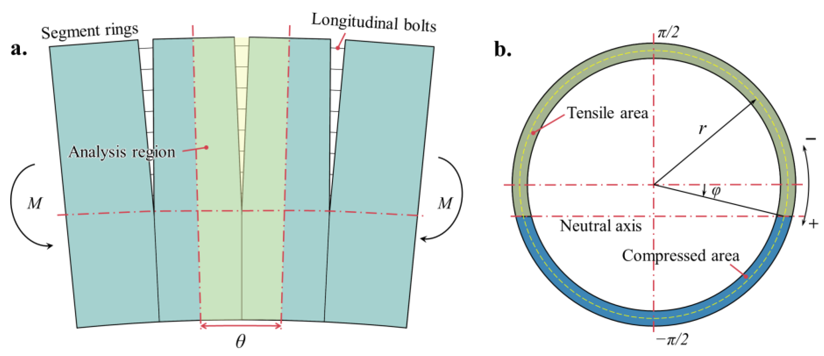
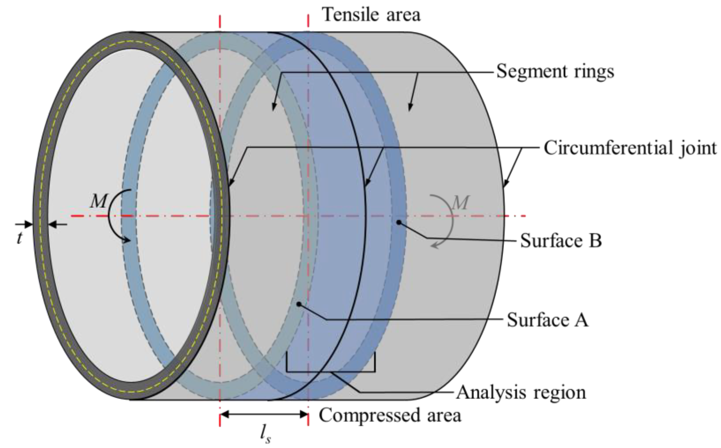
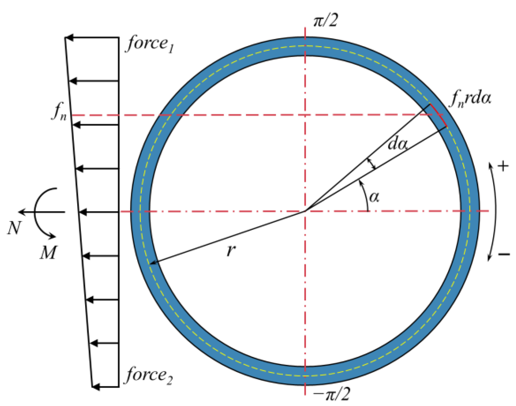
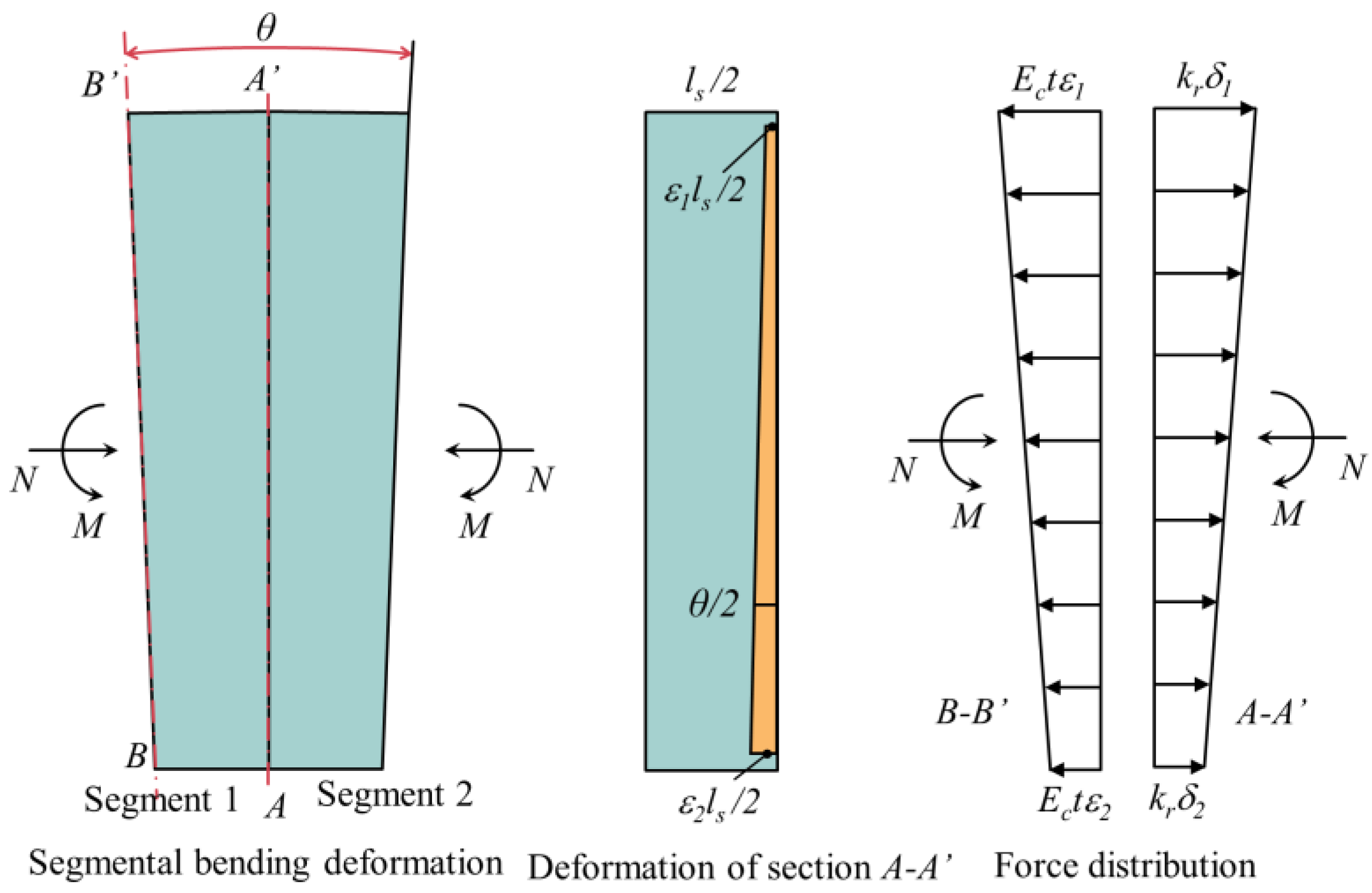
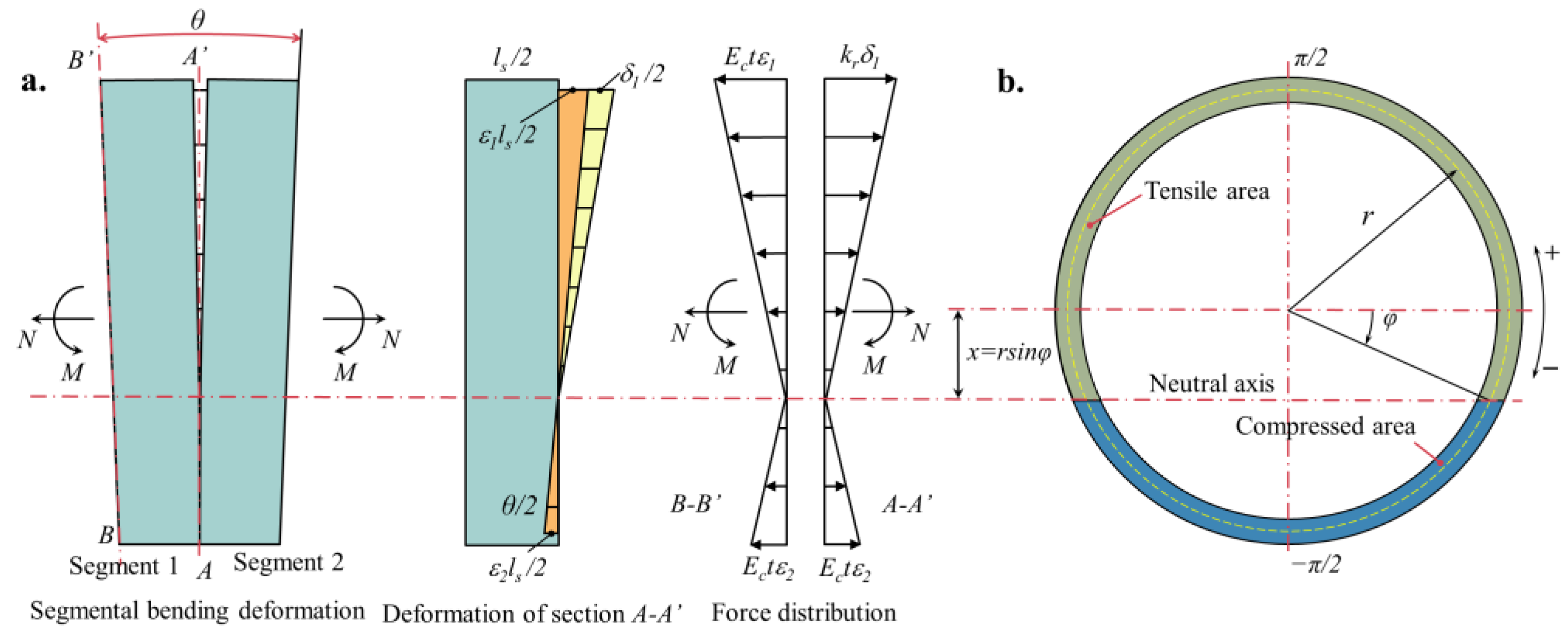
2. Longitudinal Equivalent Continuous Model

The LECM is the predominant model for shield tunnels, providing a method to calculate the equivalent bending stiffness ${EI}_{\theta eq}$ for shield tunnels when subjected to longitudinal bending moments.

When subjected to longitudinal bending moment M, the upper segmental ring stretches while the lower segment compacts (Figure 1a). The angle between the centerlines of adjacent segmental rings, known as the relative turning angle ($\theta$), the equivalent bending stiffness ${EI}_{\theta eq}$ over the analysis region $l_s$ is:

$${EI}_{\theta eq}={\displaystyle \frac{M{l}_s}{\theta }}$$

(1)

The LECM gives the expression ${EI}_{\theta eq}$ as [27]:

$${EI}_{\theta eq}={\displaystyle \frac{M{l}_s}{\theta }}=E_c{I}_s{\displaystyle \frac{{cos}^3\phi }{cos\phi +(\frac{\pi }{2}+\phi )sin\phi }}$$

(2)

where $E_c$ is the segment’s elastic modulus, Pa; $I_s$ is the moment of inertia, m⁴; $\phi$ is the neutral axis angle, rad. As shown in Figure 1b, $\phi$ satisfies the following equation:

$$\phi +cot\phi =\pi ({\displaystyle \frac{1}{2}}+{\displaystyle \frac{k_r{l}_s}{E_{c}t}})$$

(3)

where $k_r$ is the density of longitudinal bolts,$k_r={\displaystyle \frac{K_r}{2\pi r}}$, N/m²; $K_r$ is the stiffness of a single longitudinal bolt, $K_r={\displaystyle \frac{{nE}_b{A}_b}{l_b}}$, N/m; $l_s$ is the width of the segment, m; $E_c$ is the elastic modulus of the segment concrete, Pa; t is the thickness of the segment, m; n is the number of bolts, $E_b$ is the elastic modulus of the bolt, Pa; $A_b$ is the bolt cross-sectional area, m²; $l_b$ is the bolt length, m.

Also, the LECM satisfies the following assumptions:

(1)

Flat cross-section assumption.

(2)

The relative position of the neutral axis in the cross-section does not change along the longitudinal direction.

(3)

The tensile side of the segmental ring and longitudinal bolts, together with the tensile force, only the compression side of the segmental ring is under pressure; longitudinal bolts are not stressed.

(4)

The preloading force of longitudinal bolts is not considered.

(5)

The discrete distribution of longitudinal bolts along the segmental ring is simplified to an equivalent continuous uniform distribution.

(6)

Both the segment and the bolts are in the elastic stage.

3. Longitudinal Nonlinear Equivalent Continuous Model

The LECM exclusively accounts for the longitudinal deformation stiffness of shield tunnels under a single-degree-of-freedom load longitudinally. However, in actual engineering projects, factors such as uneven subsidence of strata and seismic activity inevitably result in multiple internal force combinations in shield tunnels along the longitudinal direction. Therefore, using only the LECM to consider the longitudinal deformation of shield tunnels is insufficient. Considering that both the longitudinal axial force and bending moment can cause the opening of circumferential joints, making the circumferential joints prone to danger, this study deduces the longitudinal stiffness of shield tunnels under the combined action of longitudinal axial force and bending moment.

As shown in Figure 2, the relationship between two adjacent segmental rings is presented. This paper stipulates that the bending moment causes the upper part of the segment to be in tension and the lower part to be in compression. Axial tensile forces are considered positive, while axial compressive forces are negative. Displacements, strains, and other parameters are all treated as positive values.

With a minor bending moment and substantial axial tensile force, the segmental rings separate, leaving no contact between the upper and lower parts of the segment., i.e., points a and b are not in contact, defined as Mode 1. When the bending moment is small and the axial compressive force is large, both the upper and lower parts of the segmental rings are in contact, i.e., points a and b are in contact, defined as Mode 2. When the bending moment is large and the axial force is small (either positive or negative), the segmental ring’s upper part is stretched while its lower part is compressed, i.e., point a is not in contact and point b is in contact, defined as Mode 3. The characteristics of these three modes are summarized in

Table 1. Classification Table of Longitudinal Deformation Modes of the Structure.

Mode	Contact State	Bending Moment	Axial Force
1	Completely Separated	Small	Large, Tensile
2	Completely in Contact	Small	Large, Compressive
3	Partially in Contact	Large	Small, and either Tensile, Compressive, or Zero

, and the theoretical assumptions are consistent with the LECM.

3.1. Mode 1

In the presence of substantial longitudinal axial force and bending moment, Mode 1 stress analysis depicted in Figure 3 shows that adjacent A and B segmental rings separate, with more deformation in the upper part than in the lower part.

Half of segment 1 is taken for analysis (Figure 3a), and the geometry and external force in this region are symmetric about cross-section A-A’. The left region is selected to establish the mechanical equations. According to the assumption, the deformation and force distribution on cross-sections A-A’ and B-B’ of the structure are as shown in Figure 3b. The deformation at different locations is related to the distance from the center of the segmental ring. The total deformation is the sum of the bolt’s deformation and the segment’s deformation at the same height, where the segment’s deformation is calculated as the product of its strain and width. The forces shown in Figure 4 are the projections of the distributed forces on the segmental ring in a longitudinal direction in the plane of action of the bending moment.

The equilibrium equations of forces, with $\alpha$ as the angle of integration (Figure 4), are established for surfaces A and B, respectively:

$$2{\int }_{-{\displaystyle \frac{\pi }{2}}}^{{\displaystyle \frac{\pi }{2}}}[{\displaystyle \frac{E_{c}t\left({\epsilon }_1-{\epsilon }_2\right)\left(rsin\alpha +r\right)}{2r}}+E_{c}t{\epsilon }_2]rd\alpha =N$$

(4)

$$2{\int }_{-{\displaystyle \frac{\pi }{2}}}^{{\displaystyle \frac{\pi }{2}}}[{\displaystyle \frac{E_{c}t\left({\epsilon }_1-{\epsilon }_2\right)\left(rsin\alpha +r\right)}{2r}}+E_{c}t{\epsilon }_2]sin\alpha r^{2}d\alpha =M$$

(5)

$$E_c{\epsilon }_{1}t=k_r{\delta }_1$$

(6)

$$E_c{\epsilon }_{2}t=k_r{\delta }_2$$

(7)

$$N=2{\int }_{-{\displaystyle \frac{\pi }{2}}}^{{\displaystyle \frac{\pi }{2}}}{f}_{n}rd\alpha$$

(8)

$$M=2{\int }_{-{\displaystyle \frac{\pi }{2}}}^{{\displaystyle \frac{\pi }{2}}}\left(rsin\alpha \right)f_{n}rd\alpha$$

(9)

Solving Equations (4)–(7) yields:

$${\delta }_1={\displaystyle \frac{1}{\pi }}{n}_1+{\displaystyle \frac{2}{\pi }}{m}_1$$

(10)

$${\delta }_2={\displaystyle \frac{1}{\pi }}{n}_1-{\displaystyle \frac{2}{\pi }}{m}_1$$

(11)

$${\epsilon }_1={\displaystyle \frac{1}{\pi }}{n}_2+{\displaystyle \frac{2}{\pi }}{m}_2$$

(12)

$${\epsilon }_2={\displaystyle \frac{1}{\pi }}{n}_2-{\displaystyle \frac{2}{\pi }}{m}_2$$

(13)

where,

$$n_1={\displaystyle \frac{N}{2{rk}_r}}$$

(14)

$$m_1={\displaystyle \frac{M}{2r^2{k}_r}}$$

(15)

$$n_2={\displaystyle \frac{N}{2r{E}_{c}t}}$$

(16)

$$m_2={\displaystyle \frac{M}{{2r^{2}E}_{c}t}}$$

(17)

The rotation angle $\theta$, which quantifies the difference in deformation between the upper and lower parts of the segmental ring across the analyzed area, extends up to $2r$ in Mode 1, under the combined influence of axial bending moments, $\theta$ can be reached:

$$\theta ={\displaystyle \frac{1}{2r}}\left({{\epsilon }_{1}l}_s+{\delta }_1-{{\epsilon }_{2}l}_s-{\delta }_2\right)={\displaystyle \frac{2\left(m_1+m_2{l}_s\right)}{\pi r}}={\displaystyle \frac{M{l}_s(u+1)}{\pi r^3{E}_{c}t}}$$

(18)

The equivalent bending stiffness of mode 1 is derived from Equation (2):

$${EI}_1={\displaystyle \frac{M{l}_s}{\theta }}={\displaystyle \frac{M{l}_s\pi r}{2\left(m_1+m_2{l}_s\right)}}={\displaystyle \frac{\pi r^3{E}_{c}t}{u+1}}$$

(19)

$$u=E_{c}t/k_r{l}_s$$

(20)

where u is the stiffness ratio of the segment to the bolt.

In mode 1, both the upper and lower parts of the segmental ring are tensioned, and both the segment and the bolt are involved in tension. Equivalent tensile stiffness is defined as the ratio of the product of axial force and width to the deformation at the center of the segment ($\delta$), $\delta$ represents the average deformation of the segment’s upper and lower parts, calculated as follows:

$${\delta }_u={{\epsilon }_{1}l}_s+{\delta }_1$$

(21)

$${\delta }_l={{\epsilon }_{2}l}_s+{\delta }_2$$

(22)

$\delta$ can be obtained.

$$\delta ={\displaystyle \frac{1}{2}}\left({{\delta }_u+\delta }_l\right)={\displaystyle \frac{1}{2}}\left({{\epsilon }_{1}l}_s+{\delta }_1+{{\epsilon }_{2}l}_s+{\delta }_2\right)={\displaystyle \frac{N{l}_s(u+1)}{2\pi \mathrm{r}{E}_{c}t}}$$

(23)

Then the equivalent tensile stiffness of mode 1 is:

$${EA}_1={\displaystyle \frac{2N{l}_s}{{{\epsilon }_{1}l}_s+{\delta }_1+{{\epsilon }_{2}l}_s+{\delta }_2}}={\displaystyle \frac{2\pi \mathrm{r}{E}_{c}t}{u+1}}$$

(24)

3.2. Mode 2

In mode 2, the joint interface is closed, the segment is compressed, and the internal force of the bolt is 0, with ${\delta }_1={\delta }_2=0$. The force analysis of mode 2 is shown in Figure 5. The axial force is larger, and the adjacent segmental rings A and B are compacted; the bending moment is smaller, so that the segmental ring tends to be tensile in the upper part and compressed in the lower part. Due to the bending moment, the upper part of the segment deforms more than the lower part, resulting in a rotation angle $\theta$.

Establish the equilibrium equations for either side A or B.

$$2{\int }_{-{\displaystyle \frac{\pi }{2}}}^{{\displaystyle \frac{\pi }{2}}}[{\displaystyle \frac{E_{c}t\left({\epsilon }_1-{\epsilon }_2\right)\left(rsin\alpha +r\right)}{2r}}+E_{c}t{\epsilon }_2]rd\alpha =N$$

(25)

$$2{\int }_{-{\displaystyle \frac{\pi }{2}}}^{{\displaystyle \frac{\pi }{2}}}[{\displaystyle \frac{E_{c}t\left({\epsilon }_1-{\epsilon }_2\right)\left(rsin\alpha +r\right)}{2r}}+E_{c}t{\epsilon }_2]\left(rsin\alpha \right)rd\alpha =M$$

(26)

Solving Equations (25) and (26) yields:

$${\epsilon }_1={\displaystyle \frac{1}{\pi }}{n}_2+{\displaystyle \frac{2}{\pi }}{m}_2$$

(27)

$${\epsilon }_2={\displaystyle \frac{1}{\pi }}{n}_2-{\displaystyle \frac{2}{\pi }}{m}_2$$

(28)

The common range of action in M and N in mode 2 is 2r, ${\delta }_1={\delta }_2=0$.

$$\theta ={\displaystyle \frac{1}{2r}}\left({{\epsilon }_{1}l}_s-{{\epsilon }_{2}l}_s\right)={\displaystyle \frac{2m_2{l}_s}{\pi r}}$$

(29)

The equivalent bending stiffness of mode 2 is derived from Equation (2):

$${EI}_2={\displaystyle \frac{M{l}_s}{\theta }}={\displaystyle \frac{M{l}_s\pi r}{2m_2{l}_s}}=\pi r^3{E}_{c}t$$

(30)

In mode 2, both the upper and lower parts of the segmental ring undergo compaction, involving only the segment in compression, with deformations as follows:

$${\delta }_{\mathrm{u}}={{\epsilon }_{1}l}_s$$

(31)

$${\delta }_{\mathrm{l}}={{\epsilon }_{2}l}_s$$

(32)

$$\delta ={\displaystyle \frac{1}{2}}\left({{\delta }_{\mathrm{u}}+\delta }_{\mathrm{l}}\right)={\displaystyle \frac{1}{2}}\left({{\epsilon }_{1}l}_s+{{\epsilon }_{2}l}_s\right)={\displaystyle \frac{N{l}_s}{2\pi \mathrm{r}{E}_{c}t}}$$

(33)

The equivalent compressive stiffness for mode 2 is:

$${EA}_2={\displaystyle \frac{N{l}_s}{\delta }}={\displaystyle \frac{N{l}_{s}2\pi \mathrm{r}{E}_{c}t}{N{l}_s}}=2\pi \mathrm{r}{E}_{c}t$$

(34)

3.3. Mode 3

The state of mode 3 is between mode 2 and mode 1. The axial force is small and the bending moment cannot be neglected, so the upper part of the segmental ring is pulled apart and the lower part is compacted, and the two parts are divided by the neutral axis in the middle, as shown in Figure 6.

For mode 3, the upper bolts in the upper part are stressed together with the segment in tension, and when the lower part is compressed, only the segment is stressed, and the bolts are not involved in the stresses, ${\delta }_2=0$. The force analysis for mode 3 is shown in Figure 6a. Because of the presence of bending moments, the upper deformation is greater than the lower part, resulting in a greater rotation angle $\theta$. The deformation and force distribution of the structure cross-sections A and B, as shown in Figure 6b.

It can be deduced from the coordination of geometric deformations and the balance of forces:

$${\displaystyle \frac{{\epsilon }_1{l}_s+{\delta }_1}{r-rsin\phi }}=-{\displaystyle \frac{{{\epsilon }_{2}l}_s}{r+rsin\phi }}$$

(35)

$$E_c{\epsilon }_{1}t=k_r{\delta }_1$$

(36)

$$2{\int }_{\phi }^{{\displaystyle \frac{\pi }{2}}}{\displaystyle \frac{E_c{\epsilon }_{1}t}{r-rsin\phi }}\left(rsin\alpha -rsin\phi \right)rd\alpha +2{\int }_{-{\displaystyle \frac{\pi }{2}}}^{\phi }{\displaystyle \frac{E_c{\epsilon }_{2}t}{r+rsin\phi }}\left(rsin\phi -rsin\alpha \right)rd\alpha =N$$

(37)

$$\begin{gathered} 2{\int }_{\phi }^{{\displaystyle \frac{\pi }{2}}}{\displaystyle \frac{E_c{\epsilon }_{1}t}{r-rsin\phi }}{\left(rsin\alpha -rsin\phi \right)}^{2}rd\alpha -2{\int }_{-{\displaystyle \frac{\pi }{2}}}^{\phi }{\displaystyle \frac{E_c{\epsilon }_{2}t}{r+rsin\phi }}{\left(rsin\phi -rsin\alpha \right)}^{2}rd\alpha \\ =M-Nrsin\phi \end{gathered}$$

(38)

where the neutral axis angle $\phi$ is defined as shown in Figure 6. Note that here, in order to distinguish from the LECM, the positive and negative signs are in the opposite direction to those specified for the LECM. Equations (36)–(38) can be obtained:

$${\epsilon }_1=A_1^{\prime }{n}_2+m_2{A}_2^{\prime }$$

(39)

$${\epsilon }_2=A_3^{\prime }{n}_2-m_2{A}_4^{\prime }$$

(40)

$${\delta }_1=u{\epsilon }_1{l}_s$$

(41)

$$A_1^{\prime }={\displaystyle \frac{sin2\phi +2\phi +\pi }{\pi (sin2\phi +2cos\phi )}}$$

(42)

$$A_2^{\prime }={\displaystyle \frac{2\pi sin\phi +4\phi sin\phi +4cos\phi }{\pi (sin2\phi +2cos\phi )}}$$

(43)

$$A_3^{\prime }={\displaystyle \frac{sin2\phi +2\phi -\pi }{\pi (sin2\phi -2cos\phi )}}$$

(44)

$$A_4^{\prime }={\displaystyle \frac{2\pi sin\phi -4\phi sin\phi -4cos\phi }{\pi (sin2\phi -2cos\phi )}}$$

(45)

Substituting Equations (39)–(41) into Equation (35), the following equation can be obtained:

$$(4cos\phi +2\pi sin\phi +4\phi sin\phi )m_{2}u+(sin2\phi +2\phi +\pi )n_{2}u+4\pi sin\phi m_2+2\pi n_2=0$$

(46)

The lower part of the neutral axis in mode 3 is compacted and does not rotate, so the range under the joint action of the forces M and N is not 2r, the range of action is taken as $r+rsin\phi$, and ${\delta }_2=0$.

$$\theta ={\displaystyle \frac{-{{\epsilon }_{2}l}_s}{r+rsin\phi }}$$

(47)

The equivalent bending stiffness of mode 3 is derived from Equation (2):

$${EI}_3={\displaystyle \frac{M{l}_s}{\theta }}=-{\displaystyle \frac{Mr}{{\epsilon }_2}}(1+sin\phi )$$

(48)

The simplification from Equation (40) yields

$${EI}_3={\displaystyle \frac{2(1+sin\phi )r^3{E}_{c}t}{{A_4^{\prime }-A}_3^{\prime }er}}$$

(49)

In mode 3, the upper part of the segmental ring is pulled apart, and the lower part is compacted and therefore should be subtracted. The equivalent compressive stiffness is defined in modes 1 and 2.

$$\delta ={\displaystyle \frac{1}{2}}\left({{\epsilon }_{1}l}_s+{{\epsilon }_{2}l}_s+{\delta }_1\right)$$

(50)

Then the equivalent tension-compression stiffness of mode 3 is:

$${EA}_3={\displaystyle \frac{N{l}_s}{\delta }}={\displaystyle \frac{2N{l}_s}{{{\epsilon }_{1}l}_s+{{\epsilon }_{2}l}_s+{\delta }_1}}$$

(51)

Simplification yields the following equation:

$${EA}_3={\displaystyle \frac{4e{r}^2{E}_{c}t}{(1+u)\left(A_1^{\prime }er{+A}_2^{\prime }\right){+A}_3^{\prime }er{-A}_4^{\prime }}}$$

(52)

It can be found that Equation (46) is a transcendental equation about the neutral axis angle $\phi$ in $(-{\displaystyle \frac{\pi }{2}},{\displaystyle \frac{\pi }{2}})$ with no analytical solution. It needs to be solved by numerical methods. Also ${EI}_3$ and ${EA}_3$ are both related to the neutral axis angle $\phi$.

Summarizing the above modes, it can be observed that both Mode 1 and Mode 2 have constant stiffness. This means that regardless of how axial forces and moments vary, as long as the contact status between the rings remains unchanged (completely separated or completely in contact), their stiffness remains constant. For Mode 3, its stiffness variation depends on the relationship between axial forces and moments affecting the contact status between the rings.

4. Theoretical Solution and Numerical Validation of Mechanical Parameters

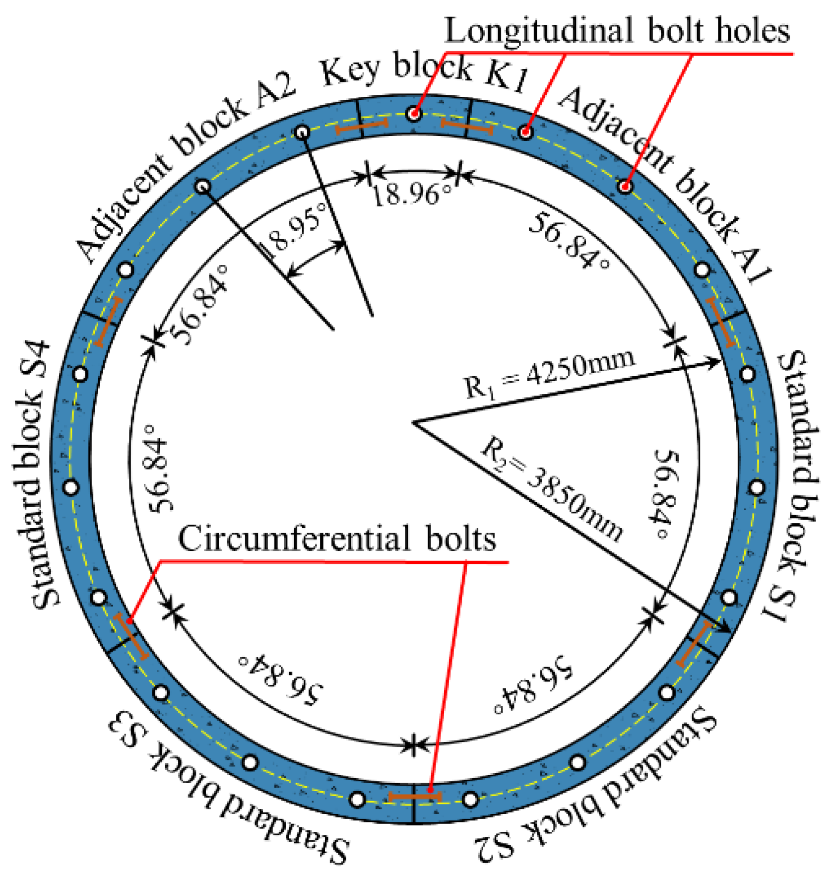
4.1. Engineering Background

The project background features Guangzhou Metro Line 18, with the segmental ring having an outer diameter of 8.5 m, an inner diameter of 7.7 m, a thickness of 0.4 m, and a width of 1.6 m. Segmental ring divided into “6+1” (18.9474° + 56.8421° × 6) blocks, consisting of 1 key block (K1), 4 standard blocks (S1, S2, S3), and 2 adjacent blocks, staggered assembly. Longitudinal and circumferential connections are made by oblique bolts, including 19 longitudinal connection bolts (M30) and 14 circumferential connection bolts (M30). The length of the bolts is 724.4 mm, and the diameter is 0.03 m. The schematic diagram of the segmental ring is shown in Figure 7.

4.2. Finite Element Modeling

ANSYS was used to establish the longitudinal analysis model of the “segmental ring-bolt” to verify the mechanical parameters of the longitudinal deformation of the shield tunnel. The solid186 element is used for the segmental ring, and the beam188 element is used for the longitudinal bolts, with longitudinal bolts embedded in the segmental rings. The targe170 and conta174 elements are used to establish contact between the segmental rings (Figure 8a), allowing for the transmission of normal and tangential forces between the segmental rings but not axial tension. At the right of the model, a fixed boundary is applied to constrain the outer interface of the segmental ring. At the left of the model, the outer interface of the segmental ring is coupled to the center point of the segmental ring, and the axial force and bending moment are applied to the center point.

Table 2. Mechanical parameters of the segment and bolt.

Items	$\mathbf{Elastic}\mathbf{Modulus}$ (GPa)
Segment (C50)	34.5
Longitudinal bolt (M30)	210

displays the parameters for the segments and bolts.

To investigate the mesh independence, 3 cases are established for numerical analysis, with element side lengths of 0.1 m (Case 1), 0.2 m (Case 2), and 0.4 m (Case 3) for the segment rings. Cases 1 and 2 result in elements on the segment thickness being at least 2 layers, whereas Case 3 results in elements on the segment thickness being 1 layer. Applying longitudinal axial forces to the model at intervals of 0.1 MN, with a maximum force of 1 MN. A small-time step size (0.05) is used for the solution, and the solution process has good stability. The system is stiff. The relationship between axial force and joint opening under different mesh partition conditions can be obtained (Figure 8b).

As seen in Figure 8b, the joint openings of the shield tunnel are consistent across different cases. Considering both the computational efficiency of the model and the rationality of stress distribution, Case 2 is chosen for subsequent analysis.

4.3. Parameter Solving and Validation

Obviously, the longitudinal bending stiffness of the shield tunnel in mode 3 is variable and related to the value of ${\displaystyle \frac{N}{M}}$. A new index, the ratio of axial force to bending moment $e={\displaystyle \frac{N}{M}}$, is introduced here as a discriminating condition for the 3 modes. In Mode 1, both the upper and lower parts of the segmental ring are pulled apart, ${\epsilon }_1$ and ${\epsilon }_2$ are positive, and the provision states that $M$ is always positive, so ${\epsilon }_1$ is always greater than ${\epsilon }_2$, ${\epsilon }_2={\displaystyle \frac{1}{\pi }}{n}_2-{\displaystyle \frac{2}{\pi }}{m}_2\ge 0$. Combining Equations (10)–(13) leads to ${\displaystyle \frac{N}{M}}\ge {\displaystyle \frac{2}{r}}$. In Mode 2, both the upper and lower parts of the segmental ring are compacted, ${\epsilon }_1$ and ${\epsilon }_2$ are negative, ${\displaystyle \frac{N}{M}}\le -{\displaystyle \frac{2}{r}}$. In Mode 3, the upper part of segmental ring is pulled apart and the lower part is compacted, ${\epsilon }_1>0$ and ${\epsilon }_2<0$, $-{\displaystyle \frac{2}{r}}\le {\displaystyle \frac{N}{M}}\le {\displaystyle \frac{2}{r}}$. In the definition, mode 3 has upper tension and lower compression. It is between modes 1 and 2 in terms of the state of force, and there is some unity with the introduced inequality relation.

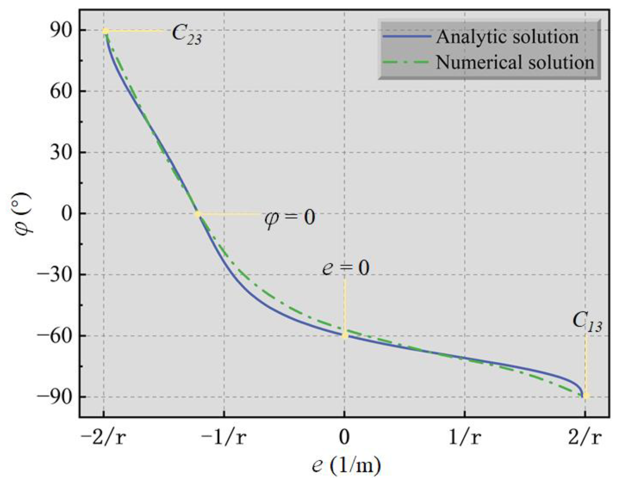
4.3.1. Neutral Axis Angle

In the longitudinal nonlinear equivalent continuous model, mode 3 gives an expression for the transcendental equation satisfied by the neutral axis angle $\phi$, as in Equation (46). When the segment is subjected only to bending moments, the axial force is 0. The $n_2$ in Equation is 0. Equation (46) can be transformed into Equation (53).

$$(4cos\phi +2\pi sin\phi +4\phi sin\phi )m_{2}u+4\pi sin\phi m_2=0$$

(53)

Simplify to obtain:

$$cot\phi +\phi =\pi \left({\displaystyle \frac{1}{u}}+{\displaystyle \frac{1}{2}}\right)$$

(54)

At this point, 1/u = −(4cosφ + 2πsinφ + 4φsinφ)/4πsinφ = −(cotφ/π + 1/2 + φ/π). Comparing with Equation (3) for calculating the neutral axis angle in the longitudinal equivalent continuous model, it can be seen that the neutral axis angle φ is constant, and 1/u can be solved as $k_r{l}_s/E_{c}t$. This implies that the longitudinal equivalent continuous model represents a specific case within the longitudinal nonlinear equivalent continuous model, specifically when the axial force is zero. At this moment, the neutral axis angle remains constant and does not vary with changes in the bending moment.

When the axial force is nonzero, combining Equations (16) and (17) helps determine the longitudinal axial force, bending moment, and other tunnel parameters. The corresponding neutral axis position angle $\phi$ is also determined. However, this is a complex equation containing several trigonometric functions, and it is difficult to obtain the solutions of $\phi$ and N, M. Moreover, the expressions of the mechanical property-related parameters such as equivalent bending stiffness, equivalent tensile stiffness, and opening are also related to$\phi$ in mode 3. During the iterative calculation, it was found that the results of Equation (46) were often difficult to converge, and the calculation was large enough to analyze the results of multiple M and N combinations. Considering that $\phi$ is both the main focus of the study and an important intermediate variable in the calculation of other parameters related to mechanical properties, and the iterative method is difficult to meet the demand, it is crucial to find a simple and convenient solution for $\phi$.

Bringing Equations (16) and (17) into (46) gives:

$$e={\displaystyle \frac{N}{M}}=-{\displaystyle \frac{(4cos\phi +2\pi sin\phi +4\phi sin\phi )u+4\pi sin\phi }{\left[\left(sin2\phi +2\phi +\pi \right)u+2\pi \right]r}}$$

(55)

When the axial force is not 0, there exists a relationship between $e={\displaystyle \frac{N}{M}}$, u, $\phi$ and, $r$ as in Equation (55).

At the critical point of the change from mode 2 to mode 3, the segmental ring is in overall contact with a tendency to separate in the upper part, i.e., the neutral axis is about to appear, at which point $\phi =-{\displaystyle \frac{\pi }{2}}$, which carries over into Equation (55) and has:

$$e_2=-{\displaystyle \frac{\left(0-2\pi +2\pi \right)u-4\pi }{\left[\left(0-\pi +\pi \right)u+2\pi \right]r}}={\displaystyle \frac{2}{r}}$$

(56)

Similarly, at the critical point of the change from mode 3 to mode 1, where most of the segmental ring is pulled apart and the last bit of contact area in the lower part is about to disappear, there will be no neutral axis, and by definition, at this point $\phi ={\displaystyle \frac{\pi }{2}}$, which carries over into Equation (56) has:

$$e_1=-{\displaystyle \frac{\left(0+2\pi +2\pi \right)u+4\pi }{\left[\left(0+\pi +\pi \right)u+2\pi \right]r}}={\displaystyle \frac{4\pi u+4\pi }{\left[2\pi u+2\pi \right]r}}=-{\displaystyle \frac{2}{r}}$$

(57)

In Mode 3, in addition to the $e_0$ point, there is a special point: during the change, when the neutral axis moves to be just at the center of the segmental ring, at which time $\phi =0$.

$$e_{\phi 0}=-{\displaystyle \frac{\left(4+0+0\right)u+0}{\left[\left(0+0+\pi \right)u+2\pi \right]r}}=-{\displaystyle \frac{4u}{(2+u)\pi r}}$$

(58)

Equation (55) is the transcendental equation. Combined with the delineation of each mode and the computational analysis in this section, it is initially believed that $\phi$ and axial bending moment ratio e have a regular correspondence. $\phi$ must be within the interval $(-{\displaystyle \frac{\pi }{2}},{\displaystyle \frac{\pi }{2}})$, and theoretically, there exist corresponding N, M at every point within the interval. Therefore, in this paper, we adopt the following treatment: Equalize the interval $(-{\displaystyle \frac{\pi }{2}},{\displaystyle \frac{\pi }{2}})$ and take 300,000 values of $\phi$ and substitute them into Equation (55) to get the corresponding 300,000 values of e. Then the $\phi -e$ curve is plotted with e as the horizontal coordinate and $\phi$ as the vertical coordinate.

The $\phi -e$ curve, derived using this method and compared with the FEM, is illustrated in Figure 9.

From the beginning of Section 4.3, $-{\displaystyle \frac{2}{r}}\le {\displaystyle \frac{N}{M}}\le {\displaystyle \frac{2}{r}}$, and the transverse coordinates of the left and right endpoints in Figure 9, e, are $-{\displaystyle \frac{2}{r}}$ and ${\displaystyle \frac{2}{r}}$, and the corresponding vertical coordinates are ${\displaystyle \frac{\pi }{2}}$ and $-{\displaystyle \frac{\pi }{2}}$. When $e=-{\displaystyle \frac{2}{r}}$, $\phi ={\displaystyle \frac{\pi }{2}}$, and the upper part of the segmental ring is just compacted at this time, which is the critical point (C₂₃) of mode 2 and mode 3; When $e={\displaystyle \frac{2}{r}}$, $\phi =-{\displaystyle \frac{\pi }{2}}$, at which time the lower part of the segmental ring is just pulled apart, i.e., it is the critical point (C₁₃) of mode 1 and mode 3; When $e=-{\displaystyle \frac{4u}{(2+u)\pi r}}$, $\phi =-{\displaystyle \frac{\pi }{2}}$, the neutral axis angle is exactly at the center of the segmental ring; When e = 0, $\phi$ is equal to that of the longitudinal equivalent continuous model, that is, the particular value of the longitudinal nonlinear equivalent continuous model when the axial force is zero.

In Figure 9, the numerically simulated$\phi -e$ curves are consistent with the theoretical result. At the special point, $e_0$, the numerical simulation result is −57.27°, and the theoretical result is −59.66°; the numerical simulation result at point $e_{\phi 0}$ (−0.3036) is close to 0°. The theoretical result agrees with the numerical result.

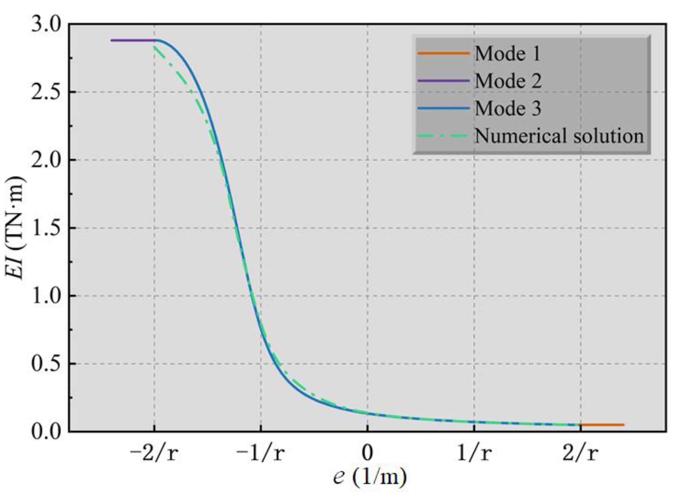
4.3.2. Longitudinal Equivalent Bending Stiffness

The longitudinal equivalent bending stiffness equations for mode 1 (Equation (19)) and mode 2 (Equation (30)) are relatively simple, and the force states are relatively clear. In mode 3, $\phi$ has been derived. When N = 0, e = 0, and Equation (49) is deformed to:

$${EI}_0={\displaystyle \frac{2(1+sin\phi )r^3{E}_{c}t}{A_4^{\prime }}}$$

(59)

Bringing Equation (45) into Equation (59) yields:

$${EI}_3={\displaystyle \frac{2(1+sin\phi )r^3{E}_{c}t\pi (sin2\phi -2cos\phi )}{2\pi sin\phi -4\phi sin\phi -4cos\phi }}$$

(60)

where the numerator can be written as $-4\pi r^3{E}_{c}t{cos}^3\phi$, and the denominator can be written as $4[-cos\phi +\left({\displaystyle \frac{\pi }{2}}-\phi \right)sin\phi ]$.

Longitudinal equivalent stiffness:

$${EI}_{\theta eq}=E_c{I}_s{\displaystyle \frac{{cos}^3\phi }{cos\phi +(\frac{\pi }{2}+\phi )sin\phi }}$$

(61)

$$I_S={\displaystyle \frac{\pi \left(D^4-d^4\right)}{64}}={\displaystyle \frac{\pi \left(8r^2+2t^2\right)\left(8rt\right)}{64}}\approx \pi r^{3}t$$

(62)

In the design of a shield tunnel, the thickness t of the segment is generally about 10% of the radius of the tunnel, and $8r^2$ is about 400 times $2t^2$, which is negligible. Therefore, $\pi r^{3}t$ can be approximated as the moment of inertia of the segmental ring, multiplied by $E_c$ which is the equivalent bending stiffness.

Then Equation (61) morphs to:

$${EI}_{\theta eq}=E_c\pi r^{3}t{\displaystyle \frac{{cos}^3\phi }{cos\phi +(\frac{\pi }{2}+\phi )sin\phi }}$$

(63)

It can be considered that the LECM is a special case of the LNECM in terms of both the neutral axis angle and the value of the equivalent bending stiffness, i.e., a special case when the axial force is zero.

From Section 3, the equations of equivalent bending stiffness in the 3 deformation modes contain the term $\pi r^3{E}_{c}t$, which is also the bending stiffness when the shield tunnel is completely under pressure. Furthermore, the problem focused on in this paper can be regarded as the coefficient problem of $\pi r^3{E}_{c}t$. Neglecting the error, the results of the derivation of the present model and the moment of inertia are numerically and formally unified. When the axial force is not 0, the e $-$EI curve is plotted in Figure 10 based on the $\phi -e$ curve according to Equation (49).

The longitudinal bending stiffness curve shows an overall decreasing trend. For the sake of discussion, it is assumed that the bending moment is constant, and the axial force is varied, resulting in a change in e.

When $e\le -{\displaystyle \frac{2}{r}}$, which is mode 2, the segmental ring is pressurized in longitudinal direction and the longitudinal bending stiffness is constant at $\pi r^3{E}_{c}t$. As the longitudinal axial pressure decreases, when $-{\displaystyle \frac{2}{r}}\le e\le e_{\phi 0}$, the longitudinal bending stiffness progressively declines, with a corresponding gradual reduction in the curve’s slope. In addition, the slope of the curve gradually decreases. As the longitudinal axial pressure decreases to 0 and then the tensile force gradually increases ($e_{\phi 0}\le e\le {\displaystyle \frac{2}{r}}$), and this interval is a concave interval. $-{\displaystyle \frac{2}{r}}\le e\le {\displaystyle \frac{2}{r}}$ belongs to mode 3, and the equivalent bending stiffness is ${\displaystyle \frac{2(1+sin\phi )r^3{E}_{c}t}{{A_4^{\prime }-A}_3^{\prime }er}}$. $\phi =0$ and $e_{\phi 0}={\displaystyle \frac{-4u}{(2+u)\pi r}}$ at the point of abrupt change between concave and convex intervals.

As the tension continues to increase, the stiffness no longer decreases when $e\ge {\displaystyle \frac{2}{r}}$ the bending stiffness is ${\displaystyle \frac{\pi r^3{E}_{c}t}{u+1}}$.

Traditional analyses of shield tunnel longitudinal stiffness frequently refer to the effective rate $\eta$, which measures the ratio of the longitudinal equivalent bending stiffness from the combined segment and bolts to the uniform continuous longitudinal stiffness under identical conditions. In mode 2, the joint is compressed, at which time only the segment is stressed, which can be regarded as a uniformly continuous model. In conventional studies, the longitudinal stiffness efficiency typically overlooks axial force effects, aligning the resulting longitudinal bending stiffness with the ${EI}_0$ value corresponding to $e=0$ in mode 3. Therefore, the longitudinal stiffness efficiency in the conventional sense is the ratio of ${EI}_0$ to ${EI}_2$, i.e., $\eta ={\displaystyle \frac{{EI}_0}{{EI}_2}}$. After the analysis in this chapter, the longitudinal stiffness efficiency is changing with $e$ all the time, and the trend is shown in Figure 11.

In conclusion, when the axial pressure significantly influences the contact status between rings more than bending moments do, the joint interfaces between the rings completely close. At this point, the longitudinal stiffness efficiency is 1.0, indicating that the longitudinal aspect of the shield tunnel can be considered a continuous reinforced concrete structure. As the axial pressure continues to decrease and transforms into gradually increasing axial tension, the longitudinal stiffness efficiency initially decreases rapidly and then gradually stabilizes. When the influence of axial tension on the contact status between rings is much greater than that of bending moments, the joint interfaces between the rings are completely open. At this point, the longitudinal stiffness efficiency becomes constant, indicating that longitudinally, the shield tunnel can be considered a discontinuous reinforced concrete structure formed by “segmental rings—fully tensioned bolts”.

4.3.3. Longitudinal Equivalent Tensile and Compressive Stiffness

In mode 1, the segmental ring is in a state of tension and bending moment, satisfying ${\displaystyle \frac{N}{M}}\ge {\displaystyle \frac{2}{r}}$, the upper and lower parts of the segmental ring are separated due to larger tension. The expression of longitudinal equivalent tensile stiffness is shown in Equation (24). In mode 2, the segmental ring is in the state of pressure and bending moment, satisfying${\displaystyle \frac{N}{M}}\le -{\displaystyle \frac{2}{r}}$, the upper and lower parts of the segmental ring are in contact due to the larger pressure, and the expression of longitudinal equivalent compressive stiffness is shown in Equation (34). In mode 3, the axial force can be either tensile or pressure, or 0, but is small relative to the bending moment, satisfying $-{\displaystyle \frac{2}{r}}\le {\displaystyle \frac{N}{M}}\le {\displaystyle \frac{2}{r}}$, the upper part of the segmental ring is separated, and the lower part is in contact, and the longitudinal equivalent tensile and compressive stiffness expression is shown in Equation (52).

The tensile and compressive stiffness are localized as:

$$EA={\displaystyle \frac{N{l}_s}{\delta }}$$

(64)

When N $=0$, $EA=0$. The parameters $u$ and $r$ of the shield tunnel have been determined, and $A_1^{\prime }~A_4^{\prime }$ are all functions of the neutral axis angle $\phi$, then ${EA}_3$ can also be interpreted as a function of $e$ and $\phi$, and the curves with $e$ on the horizontal axis and ${EA}_3$ on the vertical axis are plotted as in Figure 12.

Numerical simulations in Figure 12 generally align with the theoretical findings. The overall trend of the tensile and compressive stiffness curves is an inverse proportional function, and the transverse coordinate of the middle mutation is at$\phi =0$, i.e., $e_{\phi 0}={\displaystyle \frac{-4u}{(2+u)\pi r}}\approx -0.3036$. For discussion purposes, assume constant magnitude and direction for the bending moment, with changes in axial force altering $e$.

When $e\le -{\displaystyle \frac{2}{r}}$, which is mode 2, the segmental ring is under pressure and the longitudinal compressive stiffness is constant and constant at $2\pi \mathrm{r}{E}_{c}t$.

As the longitudinal pressure decreases, the compressive stiffness continues to increase when $-{\displaystyle \frac{2}{r}}\le e\le e_{\phi 0}$. When $e$ is close to $e_{\phi 0}$, the angle of the neutral axis of the segmental ring is close to 0°. At this time, there is an axial force but the displacement of the segment center very small and negative, so the value of the compressive stiffness increases dramatically due to the definition of stiffness. When $e$is slightly greater than $e_{\phi 0}$, the displacement of the segment center is very small but becomes positive. During this time, despite the segment pressure, under the combined action of axial force and bending moment, the displacement of the segment center is positive, leading to a phenomenon known as “negative stiffness”. The negative stiffness is concentrated in the interval $-0.3\le e\le -0.1$, corresponding to the numerical results of $-11.8TN·m\le EA\le -0.006TN·m$. As the pressure decreases to 0 (e increases to 0), the absolute value of the stiffness decreases because of the linear decrease in pressure, and the stiffness becomes 0 when $e=0$ (axial force is 0). After that, the longitudinal tensile force occurs, $0\le e\le {\displaystyle \frac{2}{r}}$, and the tensile stiffness continues to increase as the tensile force increases. When $-{\displaystyle \frac{2}{r}}\le e\le {\displaystyle \frac{2}{r}}$, the segmental ring is in mode 3, the equivalent tensile stiffness is ${\displaystyle \frac{4e{r}^2{E}_{c}t}{(1+u)\left(A_1^{\prime }er{+A}_2^{\prime }\right){+A}_3^{\prime }er{-A}_4^{\prime }}}$.

When the tension continues to increase, $e\ge {\displaystyle \frac{2}{r}}$, the longitudinal stiffness no longer changes, and the tensile stiffness is constant at ${\displaystyle \frac{2\pi \mathrm{r}{E}_{c}t}{u+1}}$.

It is evident that the tensile stiffness in Mode 1 is less than the compressive stiffness in Mode 2, and both are constants, determined by the unchanged contact status between the rings. In Mode 3, the stiffness changes with the relative relationship between axial force and bending moment. When $e$ is slightly greater than $e_{\phi 0}$, the displacement at the center of the segment becomes very small but positive. Despite the segment being under compression at this point, due to the combined action of axial force and bending moment, the displacement at the segment center becomes positive, thus resulting in “negative stiffness”.

5. Conclusions

Shield tunnels exhibit obvious discontinuities in the longitudinal direction. The conventional longitudinal equivalent continuous model can only consider the longitudinal stiffness of the shield tunnel when it is loaded by a single degree of freedom, which cannot well characterize its longitudinal deformation under the combined action of multiple internal forces. This paper derives and analyzes the longitudinal nonlinear equivalent continuous model for shield tunnels, considering both longitudinal axial force and bending moment. This study confirms that the traditional equivalent continuous model is a specific instance of the proposed longitudinal nonlinear equivalent continuous model when the axial force is zero.

According to the contact state of the joint interface of shield tunnels when longitudinal bending moments and axial forces co-exist, the longitudinal deformation of shield tunnels can be categorized into three modes, i.e., total separation of the joint interface, total contact, and partial contact. The ratio of axial force to bending moment $e$ can be used as a variable to distinguish each mode. The longitudinal equivalent bending stiffness is constant in modes 1 and 2, and in the $EI-e$ curve, modes 1 and 2 behave as straight lines at both ends of the curve. The longitudinal equivalent bending stiffness decreases with increasing $e$ in mode 3, and mode 3 is smoothly connected to modes 1 and 2 in the $EA-e$ curve. The longitudinal tension-compression stiffness is also constant in modes 1 and 2. In mode 3, there is a negative stiffness region in the longitudinal tensile stiffness, with an abrupt change at point $e_{\phi 0}$.

References

1. Liu, G.; Geng, P.; Wang, T.; Meng, Q.; Huo, F.; Wang, X.; Wang, J. Seismic vulnerability of shield tunnels in interbedded soil deposits, Case study of submarine tunnel in Shantou Bay. Ocean. Eng. 2023, 286, 115500. [Google Scholar] [CrossRef]
2. Zheng, J.; He, S.; Li, Y.; He, J.; He, J. Longitudinal Deformation of Deep Shield Tunnels Caused by Upper Load Reduction. Materials 2021, 14, 3629. [Google Scholar] [CrossRef] [PubMed]
3. Feng, K.; He, C.; Qiu, Y.; Zhang, L.; Wang, W.; Xie, H.; Zhang, Y.; Cao, S. Full-scale tests on bending behavior of segmental joints for large underwater shield tunnels. Tunn. Undergr. Space Technol. 2018, 75, 100–116. [Google Scholar] [CrossRef]
4. Wang, J.; Liu, H.; Liu, H. Measuring joint opening displacement between model shield-tunnel segments for reduced-scale model tests. Structures 2018, 16, 112–118. [Google Scholar] [CrossRef]
5. Jin, H.; Yu, S.; Zhou, S.; Xiao, J. Research on Mechanics of Longitudinal Joint in Shield Tunnel by the Nonlinear Spring Equivalent Method. KSCE J. Civ. Eng. 2019, 23, 902–913. [Google Scholar] [CrossRef]
6. Shiba, Y.; Kawashima, K.; Obinata, N.; Kano, T. Evaluation procedure for seismic stress developed in shield tunnels based on seismic deformation method. Proc. Civ. Soc. 1989, 1989, 385–394. [Google Scholar] [CrossRef] [PubMed]
7. Guo, X.; Geng, P.; Wang, Q.; Chen, C.; Tang, R.; Yang, Q. Full-scale test on seismic performance of circumferential joint of shield-driven tunnel. Soil Dyn. Earthq. Eng. 2021, 151, 106957. [Google Scholar] [CrossRef]
8. Zhang, J.; He, C.; Geng, P.; He, Y.; Wang, W.; Meng, L. Shaking table tests on longitudinal seismic response of shield tunnel through soft-hard stratum junction. Yanshilixue Yu Gongcheng Xuebao/Chin. J. Rock Mech. Eng. 2017, 36, 68–77. [Google Scholar] [CrossRef]
9. Wang, J.; Liu, H.; Liu, H.; Zou, Y. Centrifuge model study on the seismic responses of shield tunnel. Tunn. Undergr. Space Technol. 2019, 92, 103036. [Google Scholar] [CrossRef]
10. Li, X.; Zhou, X.; Hong, B.; Zhu, H. Experimental and analytical study on longitudinal bending behavior of shield tunnel subjected to longitudinal axial forces. Tunn. Undergr. Space Technol. 2019, 86, 128–137. [Google Scholar] [CrossRef]
11. Dong, Z.; Kuo, C.; Yin, J.; Wen, S.; Liu, G.; Gou, Y. Examination of Longitudinal Seismic Vulnerability of Shield Tunnels Utilizing Incremental Dynamic Analysis. Front. Earth Sci. 2021, 9, 779879. [Google Scholar] [CrossRef]
12. Lu, Y.; Song, Y.; Wang, Y.; Yuan, J. Three-Dimensional Nonlinear Seismic Response of Shield Tunnel Spatial End Structure. Adv. Civ. Eng. 2021, 2021, 8441325. [Google Scholar] [CrossRef]
13. Zhang, W.; Zhang, Q.; Cao, W. Study on Stress and Deformation of Bolt Joints of Shield Tunnel under Static and Seismic Action. KSCE J. Civ. Eng. 2021, 25, 3146–3159. [Google Scholar] [CrossRef]
14. Zhang, G.; Zhang, W.; Qi, J.; Niu, R.; Zhang, C. Seismic Response Analysis of Anchor Joint in Shield–Driven Tunnel Considering Soil–Structure Interaction. Appl. Sci. 2022, 12, 6362. [Google Scholar] [CrossRef]
15. Zhang, S.; Yang, Y.; Yuan, Y.; Li, C.; Qiu, J. Experimental investigation of seismic performance of shield tunnel under near-field ground motion. Structures 2022, 43, 1407–1421. [Google Scholar] [CrossRef]
16. Zhang, J.; Yuan, Y.; Bao, Z.; Yu, H.; Bilotta, E. Shaking table tests on shaft-tunnel junction under longitudinal excitations. Soil Dyn. Earthq. Eng. 2020, 132, 106055. [Google Scholar] [CrossRef]
17. Guo, W.; Feng, K.; Lu, X.; Qi, M.; Liu, X.; Fang, Y.; He, C.; Xiao, M. Model test investigation on the longitudinal mechanical property of shield tunnels considering internal structure. Tunn. Undergr. Space Technol. 2023, 140, 105293. [Google Scholar] [CrossRef]
18. Liu, J.; Shi, C.; Wang, Z.; Lei, M.; Zhao, D.; Cao, C. Damage mechanism modelling of shield tunnel with longitudinal differential deformation based on elastoplastic damage model. Tunn. Undergr. Space Technol. 2021, 113, 103952. [Google Scholar] [CrossRef]
19. Wu, H.-N.; Shen, S.-L.; Yang, J.; Zhou, A. Soil-tunnel interaction modelling for shield tunnels considering shearing dislocation in longitudinal joints. Tunn. Undergr. Space Technol. 2018, 78, 168–177. [Google Scholar] [CrossRef]
20. Cheng, H.; Chen, R.; Wu, H.; Meng, F. A simplified method for estimating the longitudinal and circumferential behaviors of the shield-driven tunnel adjacent to a braced excavation. Comput. Geotech. 2020, 123, 103595. [Google Scholar] [CrossRef]
21. Liu, D.; Tian, C.; Wang, F.; Hu, Q.; Zuo, J. Longitudinal structural deformation mechanism of shield tunnel linings considering shearing dislocation of circumferential joints. Comput. Geotech. 2021, 139, 104384. [Google Scholar] [CrossRef]
22. Huang, W.M.; Wang, J.C.; Yang, Z.X.; Xu, R.Q. Analytical analysis of the longitudinal response of shield tunnel lining considering ring-to-ring interaction. Comput. Geotech. 2022, 146, 104705. [Google Scholar] [CrossRef]
23. Zhang, J.; He, C.; Geng, P.; He, Y.; Wang, W. Improved longitudinal seismic deformation method of shield tunnels based on the iteration of the nonlinear stiffness of ring joints. Sustain. Cities Soc. 2019, 45, 105–116. [Google Scholar] [CrossRef]
24. Geng, P.; Mei, S.; Zhang, J.; Chen, P.; Zhang, Y.; Yan, Q. Study on seismic performance of shield tunnels under combined effect of axial force and bending moment in the longitudinal direction. Tunn. Undergr. Space Technol. 2019, 91, 103004. [Google Scholar] [CrossRef]
25. Wang, Z.; Shi, C.; Gong, C.; Lei, M.; Liu, J.; Cao, C. An enhanced analytical model for predicting the nonlinear longitudinal equivalent bending stiffness of shield tunnels incorporating combined N-M actions. Tunn. Undergr. Space Technol. 2022, 126, 104567. [Google Scholar] [CrossRef]
26. Cheng, H.; Chen, R.; Wu, H.; Meng, F.; Yi, Y. General solutions for the longitudinal deformation of shield tunnels with multiple discontinuities in strata. Tunn. Undergr. Space Technol. 2021, 107, 103652. [Google Scholar] [CrossRef]
27. Shiba, Y.; Kawashima, K.; Obinata, N.; Kano, T. An evaluation method of longitudinal stiffness of shield tunnel linings for application to seismic response analyses. Doboku Gakkai Ronbunshu 1988, 1988, 319–327. (In Japanese) [Google Scholar] [CrossRef]
Figure 1. Schematic deformation of the longitudinal equivalent stiffness beam model: (a) Longitudinal deformation; (b) The tensile and compressed areas in the cross-section.
Applsci 14 06261 g001
Figure 2. Simplified illustration of shield tunnel for calculation of bending stiffness.
Applsci 14 06261 g002
Figure 3. Deformation and force distribution of the segments in Mode 1 ( ε 1 , ε 2 represent the longitudinal strains at the tunnel’s top and bottom bolts, positive under tension and negative under compression; δ 1 , δ 2 reflect the deformation at the top and bottom bolts, respectively, always positive as these bolts endure only tension): (a) Completely separated; (b) Longitudinal stress distribution.
Applsci 14 06261 g003
Figure 4. Integral variable α .
Applsci 14 06261 g004
Figure 5. Deformation and force distribution of segments in mode 2.
Applsci 14 06261 g005
Figure 6. Deformation and force distribution of segments in mode 3: (a) Partially in contact; (b) The tensile and compressed areas in the cross-section.
Applsci 14 06261 g006
Figure 7. Segment ring cross-section schematic.
Applsci 14 06261 g007
Figure 8. Finite element model: (a) Segment model; (b) Relationship between mesh and joint opening.
Applsci 14 06261 g008
Figure 9. Comparison of analytic and numerical solutions for φ e curve.
Applsci 14 06261 g009
Figure 10. Comparison of analytic and numerical solutions for E I e curve.
Applsci 14 06261 g010
Figure 11. η e curve.
Applsci 14 06261 g011
Figure 12. Comparison of analytic and numerical solutions for E A e curve.
Applsci 14 06261 g012