HLFSRNN-MIL: A Hybrid Multi-Instance Learning Model for 3D CT Image Classification

Abstract

At present, many diseases are diagnosed by computer tomography (CT) image technology, which affects the health of the lives of millions of people. In the process of disease confrontation, it is very important for patients to detect diseases in the early stage by deep learning of 3D CT images. The paper offers a hybrid multi-instance learning model (HLFSRNN-MIL), which hybridizes high-low frequency feature fusion (HLFFF) with sequential recurrent neural network (SRNN) for CT image classification tasks. Firstly, the hybrid model uses Resnet-50 as the deep feature. The main feature of the HLFSRNN-MIL lies in its ability to make full use of the advantages of the HLFFF and SRNN methods to make up for their own weakness; i.e., the HLFFF can extract more targeted feature information to avoid the problem of excessive gradient fluctuation during training, and the SRNN is used to process the time-related sequences before classification. The experimental study of the HLFSRNN-MIL model is on two public CT datasets, namely, the Cancer Imaging Archive (TCIA) dataset on lung cancer and the China Consortium of Chest CT Image Investigation (CC-CCII) dataset on pneumonia. The experimental results show that the model exhibits better performance and accuracy. On the TCIA dataset, HLFSRNN-MIL with Residual Network (ResNet) as the feature extractor achieves an accuracy (ACC) of 0.992 and an area under curve (AUC) of 0.997. On the CC-CCII dataset, HLFSRNN-MIL achieves an ACC of 0.994 and an AUC of 0.997. Finally, compared with the existing methods, HLFSRNN-MIL has obvious advantages in all aspects. These experimental results demonstrate that HLFSRNN-MIL can effectively solve the disease problem in the field of 3D CT images.

1. Introduction

In the description of classical image classification problems based on machine learning, images typically belong to a specific category. However, in some practical scenarios, a label is assigned after observing multiple images. This process is analogous to analyzing a video, where the judgment is made only after a comprehensive view. This scenario aligns with the general concept of multi-instance learning (MIL). In 1997, Dietterich et al. proposed the concept of multi-instance learning to address the challenge of drug activity prediction. They employed the axis-parallel rectangle (APR) learning algorithm in conjunction with multi-instance learning to tackle this issue. Within the framework of multi-instance learning, a method for handling weakly supervised problems is elucidated. In this process, labels are not assigned to individual samples. Instead, based on the problem’s specifications, a subset of instances (samples) meeting the problem’s criteria is grouped into a bag, and a label is then assigned to each bag. If at least one positive instance exists within a bag, the label of the bag is defined as positive; otherwise, if all instances are negative, the bag is considered negative [1]. The primary advantage of multi-instance learning lies in its simplification of dataset construction for the respective problem, thereby reducing the workload for professionals. This advantage is particularly pronounced in medical imaging tasks, such as computer histopathology, X-ray imaging, or CT imaging screening. Given the potential existence of various associations and features among different image data, organizing these related images into bags enables multi-instance learning to better capture this information. Consequently, this approach enhances the performance and accuracy of the model [2].

Currently, numerous medical models rely on multi-instance learning frameworks to predict bag labels. Another crucial task involves assigning prediction weights to the outcomes within the bag. This process helps identify key instances that contribute to the bag label, which holds significant importance in certain medical clinical tasks. It plays a pivotal role in enabling doctors to locate the disease and formulate precise treatment plans accordingly [3]. To address this challenge, researchers have proposed various solutions. One approach involves making judgments based on the similarity at the bag level. This method utilizes the difference vector between the bag and all other bags as the feature representation, followed by prediction using this representation [4]. Another method entails embedding all instances within a bag into a compact representation, subsequently employing a bag-level classifier for prediction [5]. The third approach involves predicting low-dimensional embedded features via an instance-level classifier [6]. Among these methods, only the third can offer interpretable results. However, many researchers note that the instance-level classifier often exhibits lower prediction accuracy compared to the bag-level classifier [7]. Furthermore, in cases where there is a strong correlation among instances, employing this method may lead the model to detect abnormalities in different data segments with minor variations in the training data. Consequently, this can result in discrepancies in disease localization [8].

Computed tomography (CT) scan images currently serve as an effective method for clinically examining various diseases, including lung tumors, pneumonia, and others. According to the American Cancer Society, patients detected with lung cancer at an early stage through CT scan images have a 47% survival rate, while 80% of patients can be accurately diagnosed and treated at the central or advanced stages of cancer. A notable feature of CT scan images is their unobtrusiveness. The scanning process is relatively quiet, and compared to other imaging techniques like parallel imaging, changes in angles seldom draw attention [9]. When X-rays capture parts with a 3D structure, they are projected onto a 2D view. In some severe cases, this method may not offer effective information for professional radiologists. This is because the geometric structure overlaps during the projection process, leading to confusion regarding the actual structure. Therefore, the reconstruction of 3D scan images emerges as the preferred solution for visualizing the structural information of the patient’s lesion site, facilitating clinical analysis [10]. Three-dimensional CT scan images exhibit high-resolution features. Presently, the thickness of high-resolution CT scans can range from 1 to 1.5 mm, enabling clear observation of tissue structures and lesion sites. Typically, a single scan generates dozens to hundreds of slices based on the patient’s condition. However, disease diagnosis based on CT images relies on analyzing various permutations and combinations of features. This task proves exceedingly challenging even for experienced physicians. In recent years, the advancement of artificial intelligence and deep learning has significantly contributed to image classification. This technology has matured substantially, capable of extracting subtle features imperceptible to the human eye from different angles. Common examples include histogram features, texture features, shape features, and more [11].

The features of 3D CT scan images can be categorized into high-frequency and low-frequency features. High-frequency features typically represent fine structures within the image, such as edges and textures. These features correspond to rapidly changing or high-gradient areas in the image, such as object boundaries or structural textures. In CT images, they may manifest as clear contours, small tissue structures, or subtle tissue changes. On the other hand, low-frequency features usually depict the overall shape of the image, encompassing wide-ranging density changes or major tissue structures. These features correspond to slowly changing or low-gradient regions in the image, such as the overall shape or density distribution of the tissue. In CT images, low-frequency features may appear as the general organ shape and variations in tissue density across a wide area. CT images offer diverse levels of feature information at both high and low frequencies. However, accurately discerning these features necessitates considerable time and expertise from professional doctors [12]. In a 3D CT image, multiple adjacent slices typically comprise the image. The spacing between these slices must be carefully set to ensure that the patient’s disease information is not lost. In three-dimensional space, adjacent slices often overlap to some extent, ensuring the continuity of tissue structure within the CT image. This continuity entails seamless connection and smooth transition between adjacent slices, allowing for the reflection of spatial changes at the lesion site. Such continuity is crucial for doctors to make accurate diagnoses [13].

In this paper, our objective is to address the practical significance of CT image classification using the concept of multi-instance learning. We meticulously consider the fusion of high- and low-frequency features, as well as the continuity of 3D CT images, aiming to demonstrate its applicability in medical imaging through instances of 3D CT image data. Our experiments will evaluate two extensive public datasets focusing on lung cancer (TCIA) and pneumonia (CCII-CC), aiming to substantiate the superiority of our model over other methods. 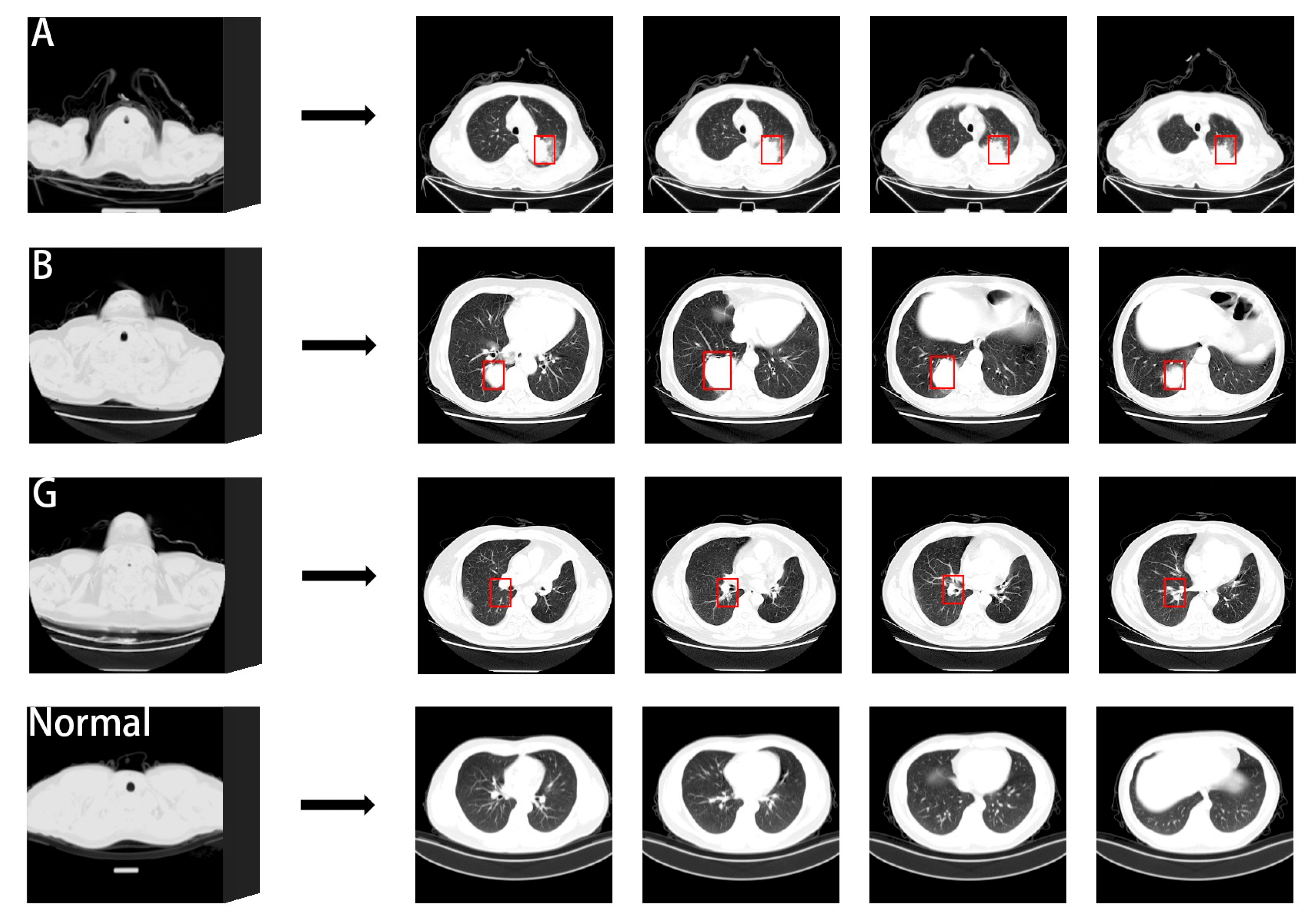Figure 1 illustrates the comparison of CT slices depicting normal lungs and three types of lung cancer from the dataset utilized in this study. Many medical experts assert that scanning a greater number of CT images decreases the risk of misjudging cancer during examinations. However, CT scan images often contain extensive nodule information. Assessing a larger number of images poses a considerable challenge but is crucial for accurate diagnosis [14].

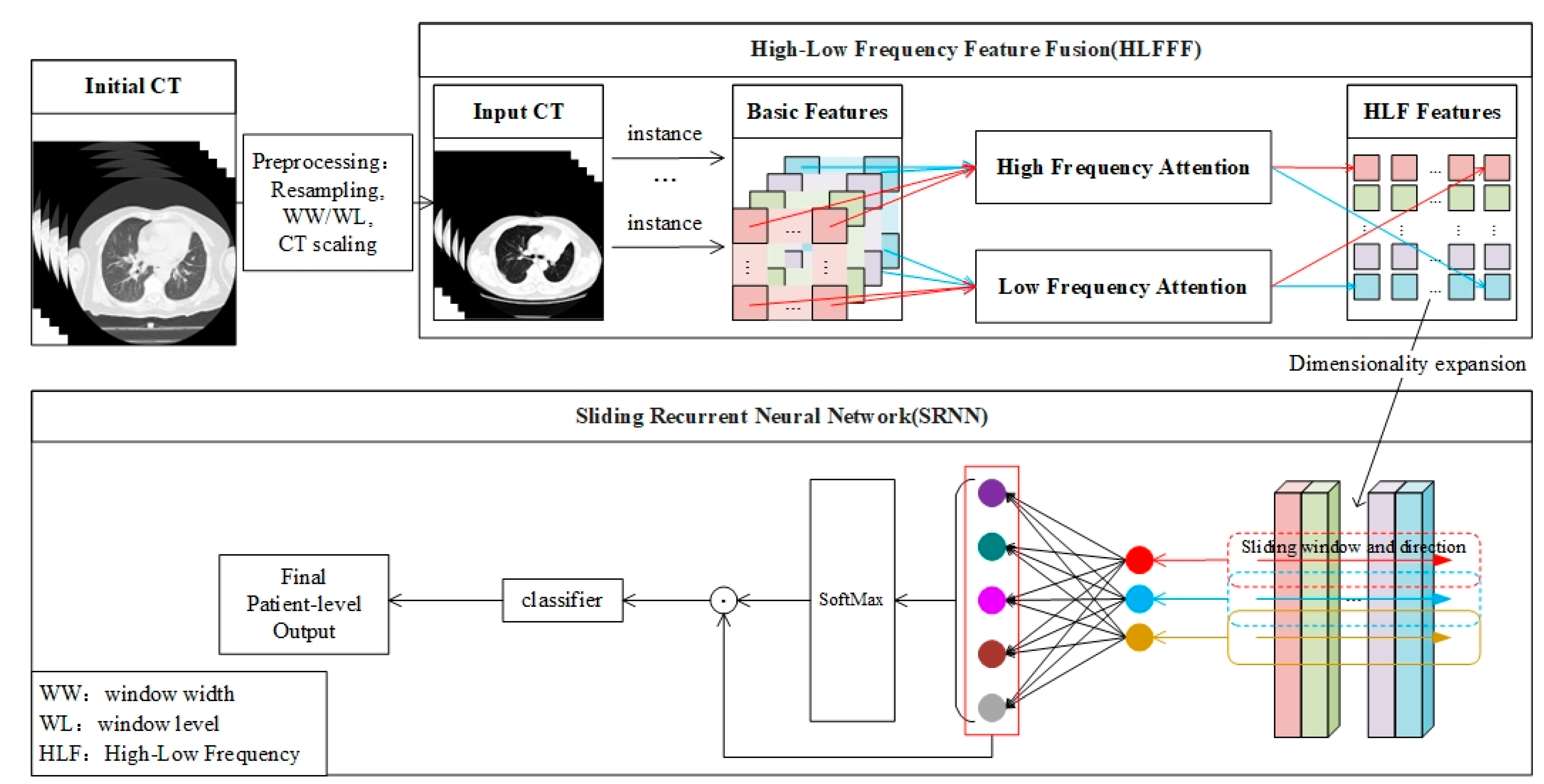
In the study, to classify CT images into lung cancer patient and normal categories, we propose a multi-instance learning model called the High–Low Frequency Sliding Recurrent Neural Network (HLFSRNN-MIL) to assist doctors in making a diagnosis of the patient’s condition. HLFSRNN-MIL leverages the principles of multi-instance learning, and the model requires only patient-level labels as input and defines a patient’s 3D CT image as a bag. The size of each bag is determined based on the patient’s specific circumstances, typically ranging from 30 to 300 slices. Each bag undergoes basic feature extraction to obtain feature information. Subsequently, the high- and low-frequency feature information derived from these features is fused, and the prediction probability of each instance within the bag is determined using our modified recurrent neural network. Finally, this information is fed into the MIL classifier to generate bag-level predictions. The paper’s main contributions are summarized below:

• We use a wide range of preprocessing techniques to mitigate the noise in the data. In this process, resampling, grayscale standardization, noise reduction, and other technologies are used to reduce the impact of noise on training.
• The HLFFF method is used in the process of feature extraction, which can effectively capture and fuse the high- and low-frequency information from the basic feature information, and improve the sensitivity of the network to various distributions of disease data.
• The SRNN method is proposed to learn and capture the temporal relationship information in the 2D feature map. This method is based on the Long Short-Term Memory Network (LSTM), which can effectively capture the relationship information between instances and identify the sequential instance fragments that affect the prediction results (that is, the continuous instance fragments of the window size in the package).
• We propose a HLFSRNN-MIL model based on the ResNet-50 network. The model adheres to the ‘end-to-end’ architecture concept, and through experiments on TCIA and CC-CCII datasets solves the problem of disease diagnosis using 3D CT images in clinical practice.

2. Related Works

In recent years, numerous models based on various algorithms have emerged to identify and detect specific features, aiming to overcome the limitations of standard CNN methods like AlexNet [15], Inception [16], ShuffleNet [17], and others. These models offer the flexibility to focus on different aspects of CT images by adjusting parameters. However, despite these advancements, the involvement of medical professionals remains crucial in this process, and significant limitations persist in clinical applications [18]. Hence, researchers in this field are actively exploring ways to enhance feature extraction within models. Improved feature extraction methods have the potential to facilitate accurate diagnosis by medical practitioners in clinical settings. Currently, there is a plethora of studies aimed at enhancing model performance in this domain.

Qin et al. [19] introduced a deep learning framework that integrates fine-grained features from PET and CT images. This framework utilizes a multi-dimensional attention mechanism to mitigate noise from feature information during the extraction of fine-grained features across multiple imaging modalities. Through experiments on feature fusion and attention concentration, they achieved ROC scores of 0.92 and observed more focused network attention. Raza et al. [20] proposed the Lung-EffNet framework for lung cancer CT scan image classification. By adapting the classification head of the EfficientNet model and incorporating a predictor based on transfer learning, they achieved an accuracy rate of 99.10% and ROC scores ranging from 0.97 to 0.99 on a public dataset. Compared to other CNN models, Lung-EffNet demonstrated faster training speeds, required fewer parameters, and exhibited model performance comparable to that of general practitioners. Xu et al. [21] introduced ISANET, a CNN-based classification model that integrates channel attention and spatial attention mechanisms into InceptionV3 to prioritize the lesion area. Compared to traditional models such as AlexNet, VGG-19, and MobileNetV3, ISANET achieved an accuracy of 95.25% in classifying non-small-cell lung cancer data. Siddiqui et al. [22] addressed the perceived limitations of existing methods in early cancer diagnosis, namely, low performance and long processing times. To overcome these challenges, they proposed E-DBN, a support vector machine based on the deep belief network. This method incorporates an improved Gabor filter with fewer parameters, resulting in reduced processing delays and times.

Chang et al. [23] proposed a model based on deep multi-instance learning (DMIL), which utilizes a deep convolutional neural network (CNN) as the backbone network for feature extraction. In DMIL, each instance corresponds to a path of the model input. The packet-level features obtained from three different methods—maximum pooling, convolution pooling, and attention mechanism pooling—are expressed as fully connected layers for prediction. This feature fusion technique allows for the estimation of the importance of each instance, thereby enhancing the model’s performance. Fuhrman et al. [24] used transfer learning to extract more complex and richer feature representations than untrained models. They connected MIL pooling (AMIL) based on an attention mechanism through two fully connected layers, which can evaluate influential slices in CT packages according to attention weights. The powerful classification ability of the model has great potential in clinical implementation. Tang et al. [25] proposed a shielded hard instance mining model (MHIMMIL) using Exponential Moving Average (EMA), which identifies difficult instances through the instance attention mechanism, and introduces parameter-free momentum into the Siamese structure to obtain more effective and stable instance prediction scores. Meng et al. [26] proposed an uncertainty-aware consensus-assisted multi-instance learning (UC-MIL) model to deal with any number of CT slices. Through training, a certain number of top instances that contribute the most to the label in the package are selected as the input for subsequent bag prediction. Subsequently, an adaptive bilateral adjacency matrix will be constructed to find vertex relationships at different granularity levels, and a graph inference module (BA-GCN) will be used to predict the patient’s diagnostic probability.

Xue et al. [27] proposed a multi-instance learning approach based on two-stage attention combined with transfer learning (TSA-MIL), which adjusts the attention weight of each instance by determining the distance between the key instance and the current instance. During the feature space processing, they adopted a clustering constraint method to refine the classification features, thereby enhancing the classification performance of TSA-MIL. Wang et al. [28] proposed a self-tuning module to mitigate the impact of unbalanced label distribution in positive packets. The confidence-based regularization strategy generates pseudo-labels for each weak input through prediction. By incorporating a Student–Teacher architecture, the model can leverage unlabeled data for training, thereby enhancing the model’s recognition ability in a cost-effective manner. Liu et al. [29] proposed an adversarial multi-instance learning (AdvMIL) model, which enhances the distribution estimation performance of AdvMIL by employing time-adversarial instances. This approach eliminates the necessity of fully supervised learning for data in the model, effectively reducing the computational cost of AdvMIL and enhancing the robustness of mainstream survival analysis methods. Schmidt et al. [30] introduced the Attention Gaussian Process (AGP) method in multi-instance learning, which leverages a combination of the Gaussian process and attention mechanism to predict the probability of instance-level labels. The packet-level predictions can be elucidated by the instance-level prediction results. This approach effectively ensures accurate fitting and predictive estimation performance of the model even when the data are unbalanced. Wang et al. [31] proposed an Iteratively Coupled Multi-Instance Learning (ICMIL) framework, which fine-tunes the parameters of the feature-extracted instance embedder using packet-level category information. This framework facilitates information exchange between the low-cost coupled instance embedder and the packet classifier, thus aiding in generating improved instance representations. In addressing the challenge of early clinical diagnosis of low-level characteristic symptoms, Li et al. [32] introduced a multi-instance learning framework based on a causal-driven graph neural network. This framework encodes spatial proximity and feature similarity between instances while emphasizing the causal components of instance features through a causal comparison mechanism, thus enhancing the diagnostic performance of the model.

These methods have played a significant role in advancing multi-instance learning, and a common trend among them is the exploration of more complex feature extraction techniques. Many current methods rely on feature extraction modules based on deep neural networks, such as ResNet [33], MobileNetV3 [34], and GoogleNet [35], among others. These network models have great differences in design concepts and performance. ResNet connects residual blocks through identity mapping to solve the problem of gradient explosion and vanishing in training. Using the inverted residual structure and separable convolution, MobileNetV3 reduces the required computing resources, enhances the feature relationship between channels, and further improves the performance of the model. GoogleNet uses a combination of convolution kernels of different shapes and pooling methods to extract features from multiple scales, which improves the utilization of computing resources. However, lesions in CT images often exhibit complex characteristics such as uncertain location, blurred shape, and varying sizes. Therefore, further research is necessary to effectively enhance the classification performance of multi-instance learning methods in CT image settings. This entails developing more sophisticated feature extraction methods that can accurately capture the nuanced characteristics of lesions in CT images, ultimately leading to improved diagnostic accuracy and clinical utility.

3. Proposed Methods

The designed method of HLFSRNN-MIL draws on the current popular network architecture concept, and combines more advanced and effective methods on the basis of a variety of feature extractors to solve the problem of 3D CT images. This design pattern is more conducive to training and subsequent parameter adjustment of the model, demonstrating high-intensity feature selection ability and excellent performance in multi-instance learning problems. Figure 2 shows an overview of the classification model proposed in this paper, which can be explained in three parts: (1) The preprocessing of 3D CT image data; (2) The extraction of the high- and low-frequency features (HLFFF) of the instance at the 2D level; (3) The search for key package segments for classification at the 2D and 3D levels (SRNN). To input a patient’s 3D CT image with any number of slices, the original CT data need to be preprocessed first, and then the processed data are sent to the HLFFF module to extract the high- and low-frequency features of each instance in a packet as a unit, and then the representation of the feature space is improved by increasing the dimension. Then, as the input of the proposed SRNN, SRNN learns the time information of the instance in the 3D space. It is worth noting that the output of SRNN can be considered as finding a packet fragment with a high contribution based on the size W of the sliding window, which is set to 5 according to the empirical hyperparameter $W$. The development details and detailed explanations of each part are given as follows.

3.1. 3D CT Datasets and Datasets Preprocessing

This paper will verify the feasibility of the method on two datasets, the Cancer Imaging Archive (TCIA) and the China Consortium of Chest CT Image Investigation (CC-CCII), and the number of slices per package is controlled between 30 and 300.

Table 1. Description of acquisition parameter information about TCIA and CC-CCII.

Information	TCIA	CC-CCII
Slice Thickness Range	(0.625 mm, 5 mm)	(0.625 mm, 5 mm)
Pixel Spacing Range	(0.585937, 0.841796)	(0.594, 0.826)
Smallest/Largest Image Pixel Value	0/2548	-
Initial WW Range	(0, 1600)	-
Initial WL Range	(−700, 40)	-
Manufacturer	GE MEDICAL SYSTEMS Philips SIEMENS	GE MEDICAL SYSTEMS
Series Description	Thorax Recon ThoraxRoutine	Siemens Toshiba
X-Ray Tube Current Range	(94, 450)	(69, 236)

presents the CT image acquisition parameter information of the two datasets.

TCIA is a large public dataset on lung cancer. A total of 300 3D CT packages were used for 234 patients with lung cancer, including 216 packages of adenocarcinoma, 41 packages of small-cell carcinoma, and 43 packages of squamous-cell carcinoma. Patients needed to be fasted for at least 6 h before the examination. Whole-body emission scanning was performed within 12 min after injection of 60F-FDG (18.4 MBq/kg, 44.0 mCi/kg). During the scan, the blood glucose of each patient was less than 11 mmol/L. The original CT image was composed of anisotropic voxels with different in-plane resolutions. Due to the differences between different scanners or acquisition protocols, the voxel spacing of the CT dataset was also inconsistent. To facilitate training, we resampled all medical images according to the voxel spacing information provided by the DICOM file to ensure consistent resolution. The slice thickness range was usually between 0.625 mm and 5 mm, and the scanning mode includes plane, contrast, and 3D reconstruction.

CC-CCII is a dataset of novel coronavirus pneumonia established by Zhang et al. [36], comprising both cases of novel coronavirus pneumonia (COVID-19) and cases of common pneumonia resulting from the SARS-CoV-2 virus. A total of 300 3D CT scans of COVID-19 and common pneumonia were included, with each scan acquired during the patient’s admission examination. This dataset is essential for distinguishing between COVID-19 and other types of pneumonia, providing valuable data for developing and validating diagnostic models.

Since X-ray absorption varies among different tissues or substances within the human body, Hounsfield Unit (HU) values require adjustment based on varying conditions. By referencing the absorption of water, a positive HU value signifies greater X-ray absorption by tissues or substances compared to water, while a negative HU value indicates lesser absorption than water. To delineate diverse types of abnormal tissues and lesions in the lungs, it is crucial to establish appropriate window width (WW) and window level (WL) settings to achieve clear lung features. In our experiment, we configured WW to 1050 HU and WL to −475 HU. The disparity between initial CT and modified input CT is illustrated in Figure 1.

Voxel spacing denotes the distance between adjacent volume pixels in the patient’s CT image within three-dimensional space. This spacing determines the minimum spatial unit discernible within the image. Smaller voxel spacing implies higher spatial resolution. Typically, the size of voxel spacing is governed by the parameter settings of the scanning device. In our experiment, the voxel spacing range of the original CT image data spanned from 0.585937 to 0.841796, while the spatial resolution range of the resampled images fell between 300 and 431. To streamline subsequent training processes, standardizing the resolution of all CT images becomes necessary. Hence, employing the OpenCV tool, the resolution of all images was uniformly scaled to 256 × 256.

3.2. Extraction of Deep Features

The fine-tuned ResNet-50 serves as the foundational network for the deep feature extraction process. The input channel of the ResNet-50 network was adjusted to 1, and the final global average pooling layer and fully connected layer were omitted. The retained portion functions as a feature extractor devoid of a classifier, thereby preserving the spatial structure of image features and encompassing feature information across various depth levels.

After the final layer, a series of feature maps was obtained, which represent image features at various levels within the network and encompass information at differing abstract levels. In the context of this paper’s problem, the number of channels in the last layer determined the quantity of features captured by each instance in the package across different aspects, corresponding to distinct feature extractors. The dimensions of the feature map depend on the size of the input image. Following convolution and pooling operations, the size transitions from the original 256 × 256 resolution to 8 × 8. Throughout this process, the feature map’s dimensions decreased while the semantic information contained within them increased.

In general, the process of acquiring CT images can be influenced by the scanning equipment and parameters, necessitating consideration of the model’s flexibility and generalization capability. The adapted ResNet-50 network effectively addresses these challenges, enabling adaptation to various tasks and application scenarios during subsequent processing.

3.3. Multiple Instance Learning

Unlike typical binary supervised learning problems, the objective of prediction in the Multiple Instance Learning (MIL) problem involves a collection of instances comprising numerous instances, denoted as $X=\left\{x_1,x_2,\dots ,x_K\right\}$. Instances within the collection exhibit no interdependence or ordering among each other. Throughout this process, it is presumed that the value of $K$ may vary across different collections, with a package label $Y$ associated with each collection, existing independently and denoted as $Y \in \left\{0, 1\right\}$. Traditional multi-instance learning assumes that each instance in the bag possesses an individual label $Y=\left\{y_1,y_2,\dots ,y_K\right\}$ and $y_k\in \left\{0, 1\right\}$ [37]. The assumption underlying the MIL problem can be articulated as follows:

$$Y=\left\{\begin{array}{cc}0,& iff{\displaystyle \sum _k}{y}_k=0\\ 1,& otherwise\end{array}\right.$$

(1)

However, obtaining labels at the instance level can be challenging and time-consuming in many practical scenarios. For instance, in CT images of lung cancer and COVID-19, medical professionals must examine all slices to identify lesion locations, where a lesion may span across a contiguous series of adjacent slices. Therefore, it becomes imperative to define an aggregation function $R\left(·\right)$ that aggregates the spatial features of instances within a specified range, such as:

$$A_i\left(x_a\right)=R\left(x_{a-\frac{w}{2}},\dots ,x_{a+\frac{w}{2}}\right)$$

(2)

where $A_i\left(x_a\right)$ is the result of the $a$-th instance aggregation, $i$ denotes the number of primary aggregations within the package, with $i=k-W+1$, where $W$ is a hyperparameter signifying the range requiring particular attention for the instance.

In many cases, the number of instances with actual corresponding labels in the positive bag may be limited and non-contiguous, influenced by factors such as slice thickness during CT scanning and the actual number of lesions present in the patient. Given this scenario, it becomes essential to adapt the two requisite transformation functions $f\left(·\right)$ and $g\left(·\right)$, of the prediction model for the MIL problem, as follows:

$$P\left(X\right)=g\left(f\left(\sum _i{A}_i\left(x_a\right)\right)\right)$$

(3)

In the current study, the selection of types for $f\left(·\right)$ and $g\left(·\right)$ is approached from different perspectives to address the problem [38]. Firstly, the focus lies on the instance-based method. Here, the transformation function $f\left(·\right)$ is regarded as an instance-level classifier, while $g\left(·\right)$ is considered an identity function that consolidates instance scores. While this method offers high interpretability, scholars [39] have observed its inferior effectiveness compared to the embedding-based approach across all facets. The embedding method utilizes $f\left(·\right)$ as a low-dimensional embedding feature extractor, with $g\left(·\right)$ serving as a packet-level aggregation operator. By aggregating sample-level features into packet-level features, predictions for package labels can be made.

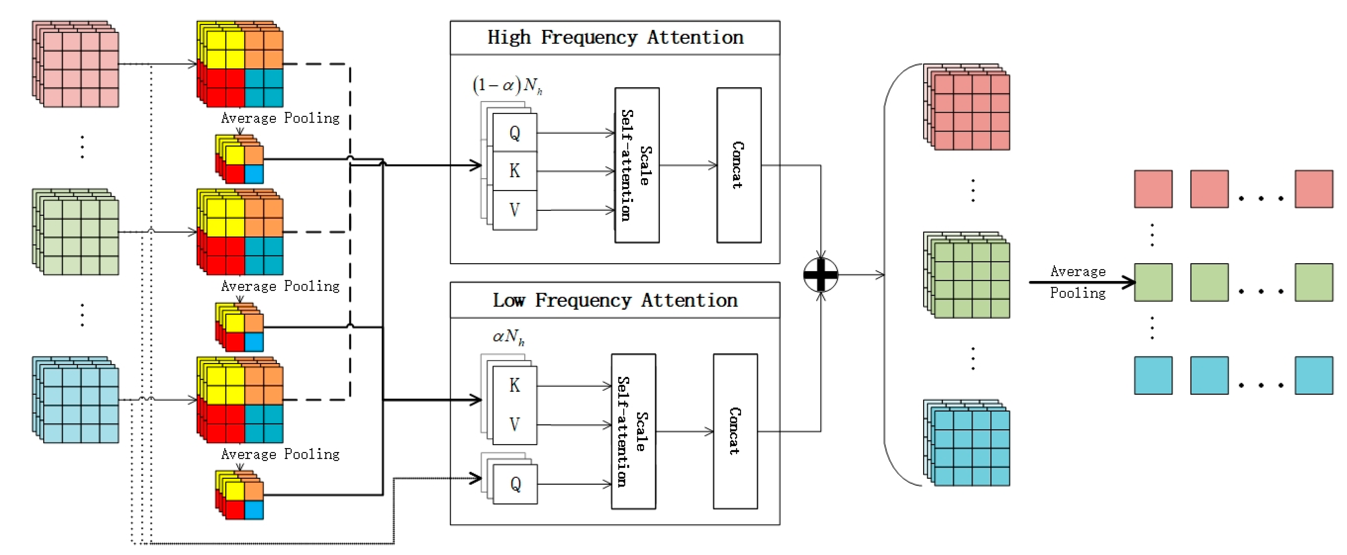
3.4. HLFFF Method for Processing High-Frequency and Low-Frequency Features

For the MIL problem parameterized by the neural network, $f\left(·\right)$ is used as a feature extractor. This paper proposes an HLFFF method that combines the basic feature extraction network with Hilo attention [40], as shown in Figure 3. In the face of the complex problems of high-resolution images, the semantic information of features can be re-added from the perspective of high frequency and low frequency. This section will explain the HLFFF method with the feature extraction network based on ResNet-50.

The output vector $M\in R^{N\times D}$ from the last residual block of ResNet-50 is preserved. Here, $M$ represents the feature matrix acquired from each instance under identical conditions, where $N$ denotes the number of instances in the package, and $D$ signifies the size of the hidden dimension. Subsequently, dimensionality reduction is applied to the feature vector of each instance, followed by global average pooling over a specified window size. The data $M$ before pooling and the data $MP$ after pooling are utilized as inputs for high-frequency attention and low-frequency attention.

Initially, leveraging the multi-head self-attention mechanism (MSA) [41], $h$ self-attention heads are designated, each assigned with Query matrices ($Q$), Key matrices ($K$), and Value matrices ($V$):

$$Q_{hi}=M_k{W}_q^h,K_{hi}=M_k{W}_k^h,V_{hi}=M_k{W}_{\nu }^h$$

(4)

$$Q_{lo}=M_k{W}_q^h,K_{lo}=M_k{W}_k^h,V_{lo}=M_k{W}_{\nu }^h$$

(5)

where $hi$ and $lo$ denote the high-frequency and low-frequency attention branches, respectively. $W_q^h,W_k^h,W_v^h\in R^{D\times D_h}$ are the attention weights that $QKV$ can learn. The input for $K_{lo}$ and $V_{lo}$ is $MP$, where $D$ represents the number of hidden weight matrices, and $D_h$ is the number of hidden weight matrices corresponding to each self-attention head. Subsequently, the weighted sum of the output vectors from each head is computed:

$$S{A}_{hi}^h\left(M_k\right)=Softmax\left(\frac{Q_{hi}{K}_{hi}^T}{\sqrt{D_h}}\right)V_{hi}$$

(6)

$$S{A}_{lo}^h\left(M_k,M{P}_k\right)=Softmax\left(\frac{Q_{lo}{K}_{lo}^T}{\sqrt{D_h}}\right)V_{lo}$$

(7)

Then, combine the output of each head:

$$Hi\left(M\right)=concat\left[S{A}_{hi}^h\left(M_k\right)\right]W_o$$

(8)

$$Lo\left(M\right)=concat\left[S{A}_{lo}^h\left(M_k,M{P}_k\right)\right]W_o$$

(9)

In the formula, $W_o\in R^{\left(N_h\times D_h\right)\times D}$ denotes a linear projection layer for series output. Here, $N_h$ represents the total number of self-attention heads in this layer, harmonizing the dimensions of output and input.

In this process, a hyperparameter $\alpha \in \left[\mathrm{0,1}\right]$ is defined to regulate the number of self-attention heads participating in high frequency and low frequency, respectively. $\alpha \times N_h$ denotes the number of self-attention heads assigned to high frequency, while $\left(1-\alpha \right)\times N_h$ denotes the number of self-attention heads allocated to low frequency. Depending on the nature of the problem at hand, the value of α can be adjusted to prioritize either high frequency or low frequency, thereby potentially reducing computational complexity to some extent.

High-frequency attention ($Hi$): The intuitive concept here involves utilizing high-frequency components to encode local details of the target. This is achieved by capturing high-frequency information through the establishment of a local self-attention window (for example, a 2 × 2 window). Low-frequency attention ($LF$): Each window employs average pooling to acquire down-sampled feature information $MP$, which is then mapped to $K_{lo}$ and $V_{lo}$, while $Q_{lo}$ utilizes the original feature information $M$. This approach not only captures abundant low-frequency information but also alleviates the complexity of Formulas (5) and (7).

Finally, the output of HLFFF is obtained through concatenating each attention result:

$$HLFFF\left(M\right)=concat\left[\begin{array}{c}Hi\left(M\right),Lo\left(M\right)\end{array}\right]$$

(10)

3.5. SRNN Method for Processing Instance with Temporal Relationships

In the classic MIL scenario, there is a fundamental assumption that each instance within a package is independent of one another. However, when a patient’s 3D CT image is employed as a MIL package, there exists a contiguous relationship between each slice. In this context, the target lesion at the same position might consecutively appear across several adjacent slices. Given that these lesions actually pertain to the same morphologically similar structure, we propose the utilization of a recurrent neural network to process a certain length of the instance sequence. In doing so, it is crucial to maintain the spatial order of instance upon input. A sequence of sequentially continuous instances is termed a sequence.

The significance of the SRNN method lies in its ability to identify an instance similarity vector that aligns with the target variations within a sequence. However, the uncertainty regarding the number of instance $k$ in each package presents a challenge. One existing approach is to employ a fixed-length sequence template. In this method, the length of the template must exceed the length of each package used. When the size of the package falls short of this length, the vacant portion is filled with zeros. However, this approach gives rise to two issues. Firstly, it can lead to inefficient utilization of computational resources when dealing with packages containing a small number of instances (with the largest package approximately 10 times the size of the smallest package). Secondly, the padding of zeros may degrade the learning performance of the network, particularly in cases of highly unbalanced data.

This paper proposes to employ a sliding window $w$ to encode sequential packages. The selection of $w$ entails additional configuration, yet within packages of varying sizes, $n$ encoded sample fragments emerge:

$$n=k-w-1$$

(11)

After such processing, the sequence length of each input to the recurrent neural network equals $w$, resulting in:

$$Fr=Se\left({HlFFF\left(M\right)}^T\right)$$

(12)

Here, $Se$ is a sliding encoder, and then the recurrent neural network uses a long short-term memory (LSTM) network. The input is a feature map obtained by the HLFFF method, as shown in Figure 4. Here, the $n$-th instance sequence obtained by $Se$ in order is considered to be the state at time $t$, and the gated unit at time $t$ is calculated by referring to the mathematical calculation formula of LSTM:

$$i_{n_t}=\sigma \left(W_{i}F{r}_{n_t}+U_i{h}_{t-1}\right)$$

(13)

$$f_{n_t}=\sigma \left(W_{f}F{r}_{n_t}+U_f{h}_{t-1}\right)$$

(14)

$$o_{n_t}=\sigma \left(W_{o}F{r}_{n_t}+U_o{h}_{t-1}\right)$$

(15)

$${\tilde{c}}_t=tanh\left(W_{c}F{r}_{n_t}+U_c{h}_{t-1}\right)$$

(16)

$$c_t=i_{n_t}\odot {\tilde{c}}_t+f_{n_t}\odot {\tilde{c}}_{t-1}$$

(17)

$$h_t=o_{n_t}\odot tanh\left(c_t\right)$$

(18)

Here, $\sigma$ represents the sigmoid function, while $W_i$, $W_f$, $W_o$, $U_i$, $U_f$, and $U_o$ denote the weight matrices that can be learned within the LSTM. ${Fr}_{n_t}$ signifies the sequence vector of the $t$-th time step of the $n$-th sequence, $h_t$ denotes the hidden state at the $t$-th time step, and $c_t$ represents the memory unit at the $t$-th time step. Particularly, $W_c$ represents the weight matrix employed to calculate the memory unit required for the next sequence. It is utilized to map the hidden state $t-1$ of the current time $t$ input ${Fr}_{n_t}$ and the previous time $t-1$ to the memory unit $c_t$ needed for the subsequent sequence.

4. Experiments and Results

In this chapter, the effectiveness of the proposed method will be validated using two large public datasets. The first dataset comprises lung cancer data from TCIA, while the second dataset is the CC-CCII dataset, which currently holds a prominent position in COVID-19 research.

4.1. Datasets and Experimental Settings

The TCIA lung cancer dataset comprises comprehensive lung cancer images updated in 2020, encompassing adenocarcinoma (A), small-cell carcinoma (B), and squamous-cell carcinoma (G). It provides DICOM format medical data files, facilitating the adjustment of imaging parameters as per specific requirements. On the other hand, the CC-CCII novel coronavirus pneumonia dataset, released in 2020, consists of 3D CT images of novel coronavirus pneumonia (NCP) and common pneumonia (CP). This dataset offers processed PNG format data files suitable for direct training.

In the experiment of this project, the learning ability and generalization ability of the proposed model will be assessed on these two datasets separately. Detailed information on the two datasets is provided in

Table 2. Description of the experimental setup for TCIA and CC-CCII.

Datasets	Classes	Slices		Bags
		Train and Val	Test	Train and Val	Test
TCIA	A	9045	2683	167	49
	B	1712	386	34	7
	G	1629	741	29	14
	Normal	15,318	4517	230	70
	Total	27,704	8327	460	140
CC-CCII	NCP	16,232	5142	230	70
	CP	12,151	3425	230	70
	Total	28,383	8567	460	140

, with the number of slices ranging from 30 to 300. The TCIA dataset comprises 36,031 slices, while the CC-CCII dataset contains 36,950 slices. To evaluate the model’s performance, a 5-fold cross-validation is employed during the training and testing phases. All packages are approximately split into training and test sets in a 4:1 ratio. During each batch’s training process, four-fifths of the training set is utilized to learn the weight parameters in the model, while the remaining one-fifth is used to assess the model’s generalization ability. The experimental results will be averaged across five experiments.

When transforming the data content into the tensor format required for the experiment, each 512 × 512 resolution CT image is scaled down to 256 × 256, representing only one-quarter of the initial CT image size. This resizing reduces the file size and training time of the training data overall, while also alleviating the demand on video memory to some extent. Importantly, there is minimal disparity between the data after model testing and the data before modification.

All experiments of this evaluation model will be conducted on a local workstation equipped with an Intel^® Core™ i9-12900H CPU and an NVIDIA GeForce RTX 3070 Ti Laptop GPU. The manufacturers of CPU and GPU are Intel and NVIDIA, both of which are purchased in China. Given the large dataset, 32 GB of memory is utilized. The initial learning rate of the model is configured to 0.0005, and subsequently, the learning rate of the Adam optimizer is decayed using the cosine annealing method. The number of training epochs for each model is set to 50.

4.2. Evaluation Metrics

The problem solved in this paper is a binary classification problem. To evaluate the performance of the classification model in practical scenarios, typical classification evaluation indicators are usually used for evaluation, including Sensitivity (SEN), Specificity (SPE), Precision, F1 score, accuracy (ACC), and area under the receiver operating characteristic (ROC) curve (AUC). Here, the area under the ROC curve is used to assess the model’s ability to predict positive and negative instances across various thresholds. When the data category distribution is unbalanced, the use of AUC and ACC can more comprehensively evaluate the comprehensive performance of the model. Different classification models are evaluated by the above six evaluation indicators:

$$SEN=\frac{TP}{TP+FN}$$

(19)

$$SPE=\frac{TN}{TN+FP}$$

(20)

$$Precision=\frac{TP}{TP+FP}$$

(21)

$$F1 score=\frac{2\times Precision\times Recall}{Precision\times Recall}$$

(22)

$$ACC=\frac{TP+TN}{TP+TN+FP+TN}$$

(23)

$$AUC={\int }_0^{1}SENd\left(\frac{FP}{FP+TN}\right)$$

(24)

In the formulas, TP represents true positives, TN represents true negatives, FP represents false positives, and FN represents false negatives. Recall is calculated in the same way as Sensitivity (SEN). By computing these six indicators on the actual dataset, we can compare them with those of currently popular models to demonstrate the effectiveness of the proposed method.

4.3. Ablation Experiments on TCIA

This paper aims to investigate the contribution of the HLFFF and SRNN methods to the classification network. The FLFFF method requires setting the value of $\alpha \in \left(\mathrm{0,1}\right)$ to adjust the weight distribution of high frequency and low frequency in the method. Initially, ResNet-50 is utilized as the fundamental feature extraction method of the model. The value of $\alpha$ is set in the range of 0.1 to 0.9, with an interval of 0.1, yielding a total of nine values. The benchmark model of ResNet-50 combined with the HLFFF method is tested on the TCIA dataset.

Table 3. Performance comparison of HLFFF method under different $\mathit{\alpha }$ values.

$\mathit{\alpha }$	AUC	ACC	SEN	SPE	F1 Score	Precision
$\alpha =0.1$	0.924	0.914	0.995	0.829	0.921	0.854
$\alpha =0.2$	0.930	0.907	0.886	0.929	0.905	0.925
$\alpha =0.3$	0.952	0.936	0.871	0.914	0.931	0.921
$\alpha =0.4$	0.932	0.943	0.996	0.886	0.946	0.897
$\alpha =0.5$	0.966	0.957	0.997	0.997	0.959	0.951
$\alpha =0.6$	0.958	0.936	0.986	0.886	0.939	0.896
$\alpha =0.7$	0.950	0.907	0.943	0.871	0.910	0.885
$\alpha =0.8$	0.919	0.893	0.998	0.786	0.903	0.824
$\alpha =0.9$	0.899	0.879	0.786	0.971	0.866	0.965

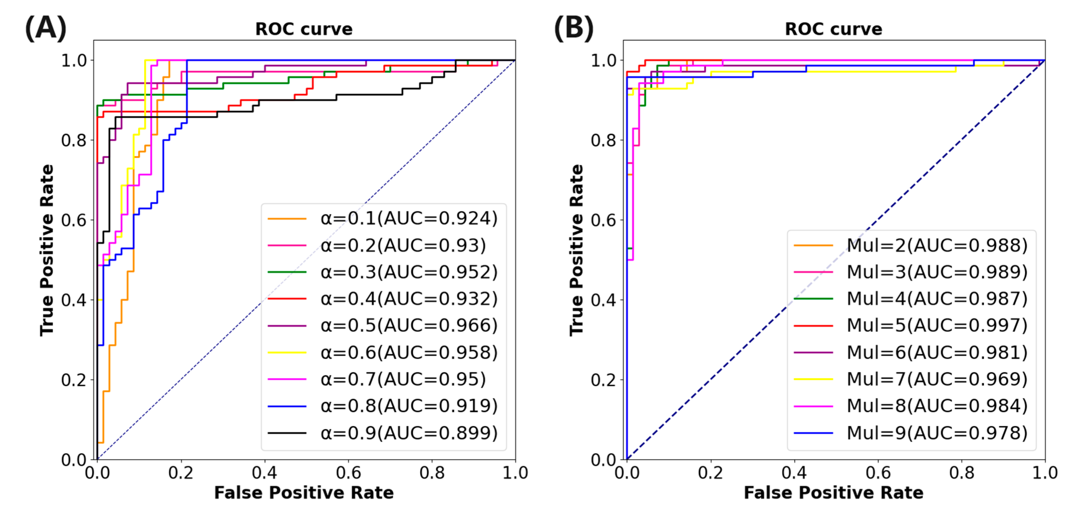
summarizes the performance indicators under different $\alpha$ values. Figure 5A illustrates the area under the ROC curve under varying $\alpha$ values. The results indicate that when $\alpha =0.5$, the model performs optimally, with the AUC and ACC increasing by 7.8% and 6.7%, respectively, compared to the classification model utilizing only ResNet-50.

The SRNN method needs to set the value of $w\in R$ to adjust the length of the instance fragment processed by the method. The experiment will be carried out on the basis of the combination of ResNet-50 and HLFFF methods. The value of $w$ is set between 2 and 9 and the interval is 1, a total of 9 values. The benchmark model combining ResNet-50 and the HLFFF and SRNN methods is also tested on the TCIA dataset.

Table 4. Performance comparison of SRNN method under different $\mathit{w}$ values.

$\mathit{w}$	AUC	ACC	SEN	SPE	F1 Score	Precision
$w=2$	0.988	0.943	0.929	0.957	0.942	0.956
$w=3$	0.989	0.951	0.986	0.914	0.952	0.920
$w=4$	0.987	0.981	0.982	0.971	0.958	0.958
$w=5$	0.997	0.992	0.995	0.997	0.995	0.995
$w=6$	0.981	0.957	0.943	0.957	0.950	0.957
$w=7$	0.969	0.950	0.929	0.971	0.949	0.970
$w=8$	0.984	0.943	0.943	0.943	0.943	0.943
$w=9$	0.978	0.921	0.843	0.885	0.903	0.915

shows the performance indicators of the model under different w values. Figure 5B shows the area under the ROC curve under different w values. The results show that the performance of the model is optimal when $w=5$, which means that each time the sample fragment with a length of five is input into the SRNN method, the AUC and ACC are increased by 3.3% and 3.5%, respectively, compared with the model using only the HLFFF method.

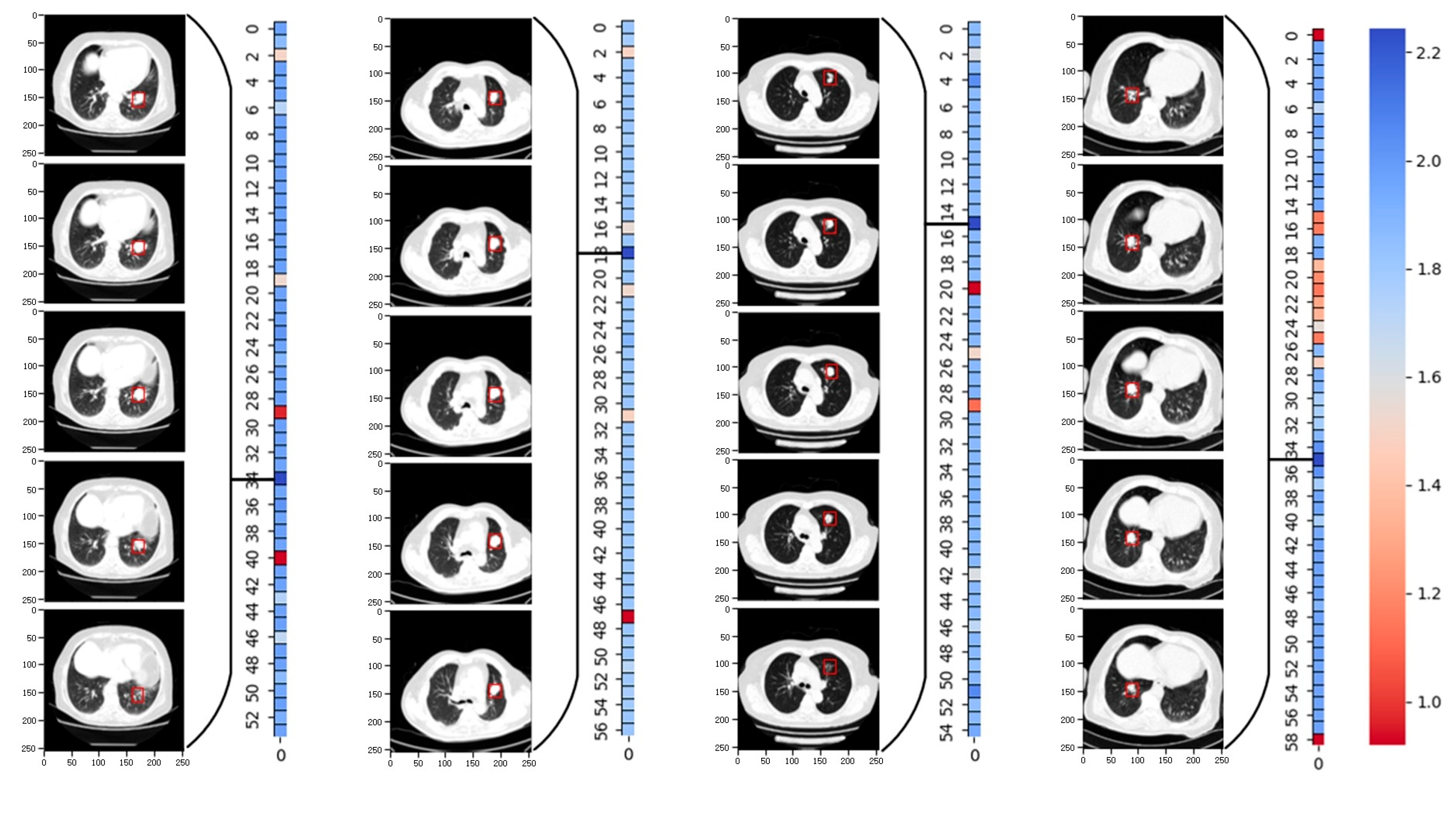
In particular, we evaluated the accuracy of the model predictions based on the le-sion site annotations in the original TCIA dataset. By generating weight heat maps for each sample fragment after applying the SRNN method, Figure 6 displays the weight heat maps for four packages. Each weight represents a fragment of length 5. The re-sults demonstrate that the SRNN method adeptly identifies the fragment with the highest lesion weight. The red boxes in the graph denote annotation boxes marked ac-cording to corresponding annotation information, highlighting the lesion sites identi-fied by the SRNN method.

4.4. HLFSRNN-MIL Method and Its Performance on TCIA

In order to eliminate the influence of the feature extraction network on the proposed method, the experiment will use the current popular feature extraction networks and the proposed method for performance evaluation.

Table 5. Comparison of various feature extraction networks used by HLFSRNN-MIL.

Feature Extraction Network	Size of Model (MB)	Initial Learning Rate	Training Time (s)	Feature Map
ResNet-50	86.0	0.0005	954/epoch	512 × 8 × 8
MobileNetV3	18.3	0.0005	768/epoch	960 × 8 × 8
DenseNet-201	7.55	0.0005	648/epoch	512 × 8 × 8
GoogleNet	41.2	0.0005	672/epoch	1024 × 8 × 8
AlexNet	442	0.0005	444/epoch	256 × 6 × 6
VGG-19	86.7	0.0005	1236/epoch	512 × 8 × 8

shows the basic information of the network used. The initial learning rate is set to 0.0005, and the learning rate reduction method is optimized by the cosine annealing algorithm.

Table 6. Performance comparison of HLFSRNN-MIL in different feature extraction networks in TCIA.

Feature Extraction Network	AUC	ACC	SEN	SPE	F1 Score	Precision
ResNet-50	0.997	0.992	0.995	0.997	0.995	0.995
MobileNetV3	0.979	0.991	0.986	0.971	0.979	0.972
DenseNet-201	0.978	0.957	0.999	0.914	0.959	0.921
GoogleNet	0.986	0.986	0.986	0.963	0.993	0.986
AlexNet	0.942	0.943	0.986	0.886	0.946	0.897
VGG-19	0.946	0.943	0.986	0.886	0.946	0.897

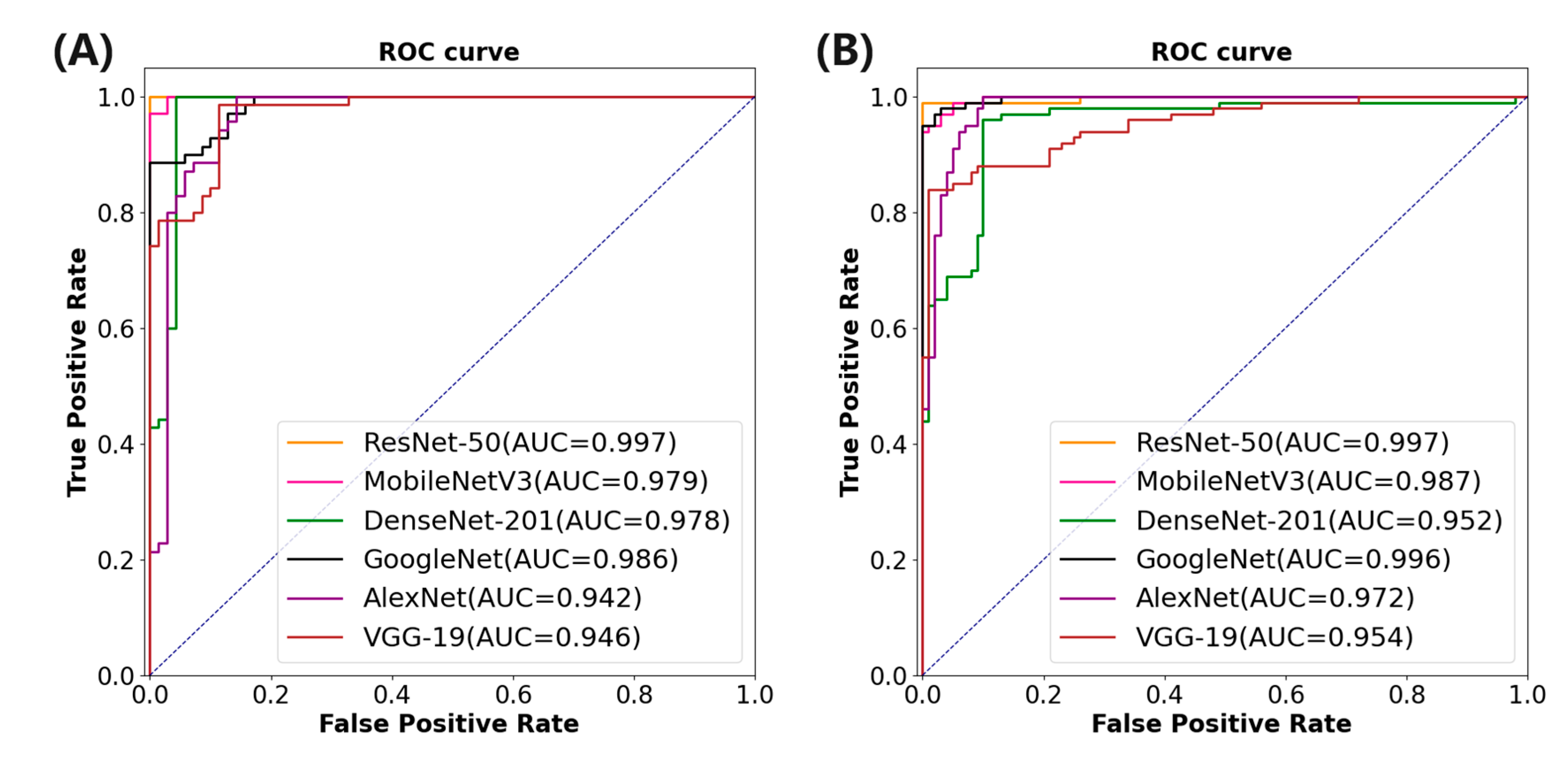
corresponding to Table 5 shows the performance index of the proposed method combined with different feature extraction networks. It is evident that although AlexNet boasts a shorter training time, its performance across all metrics is notably poorer compared to ResNet-50, which exhibits the best performance metrics. Specifically, ResNet-50 achieves an AUC of 0.997, ACC of 0.992, SEN of 0.995, SPE of 0.997, and F1 score of 0.995. Figure 7A depicts the area under the ROC curve of different feature extraction networks combined with the proposed method.

4.5. Attention Heat Maps Visualization for HLFSRNN-MIL on TCIA

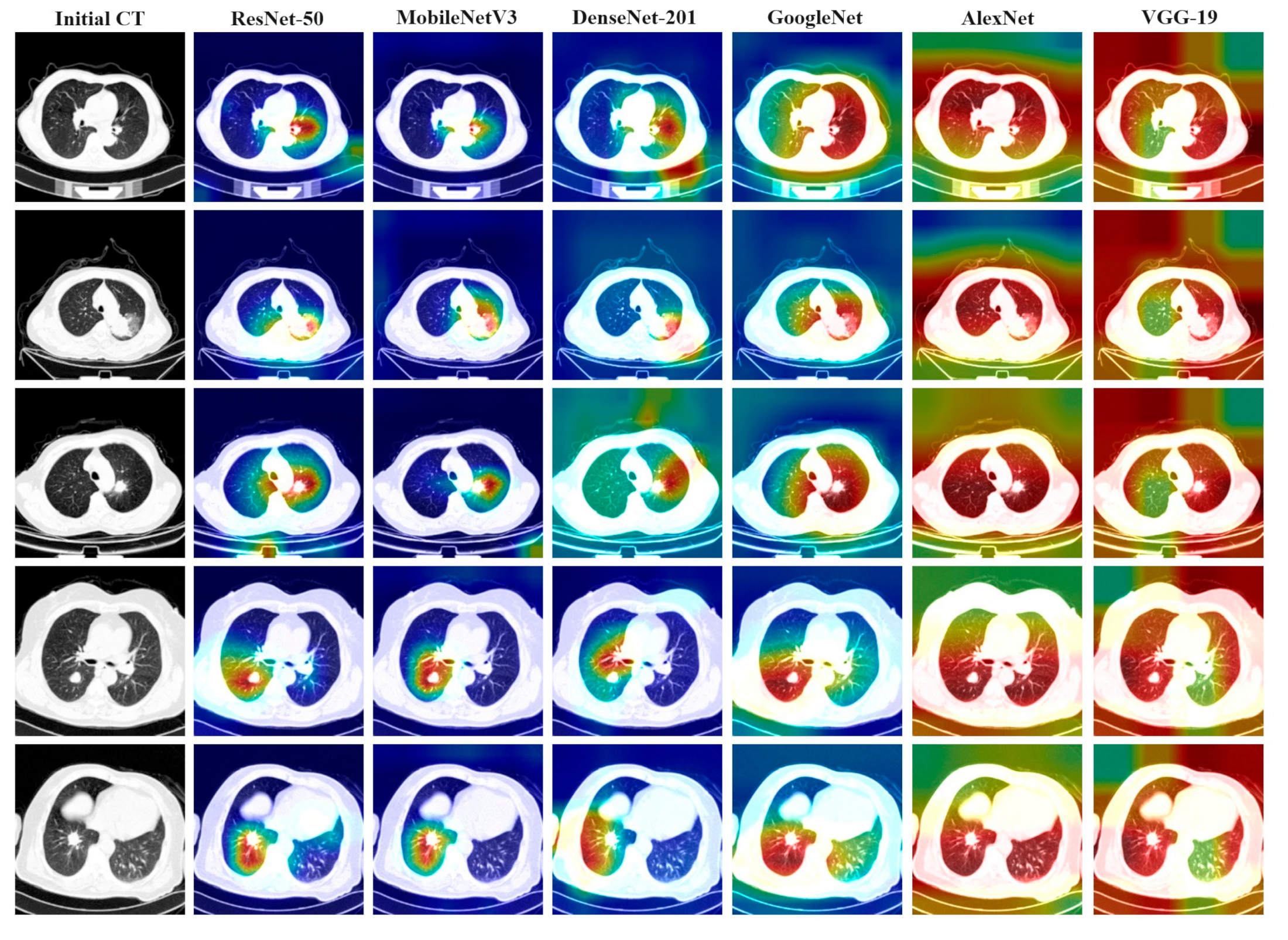
Figure 8 illustrates the thermal image generated under various conditions of different feature extraction networks, alongside the attention heat map generated by the gradient category activation mapping (Grad-CAM) method. The first column in the figure represents the result of a lung cancer patient’s slice, with each row displaying the original CT slice image and the Grad-CAM results depicted under different network models. Observations reveal that models exhibiting better performance metrics tend to focus their attention on more concentrated and accurate areas, whereas models with lower indicators often concentrate attention on areas unrelated to the lesion site. Notably, the areas of interest for ResNet-50, MobileNetV3, and GoogleNet are predominantly centered on the lesion.

4.6. Comparison of HLFSRNN-MIL with Other Methods on CC-CCII

Finally, the performance of the proposed HLFSRNN-MIL on the CC-CCII dataset is evaluated in terms of generalization and robustness. Firstly, we select the most outstanding performance indicators based on different feature extraction networks. The results are presented in

Table 7. Performance comparison of HLFSRNN-MIL in different feature extraction networks on CC-CCII.

Feature Extractor	AUC	ACC	SEN	SPE	F1 Score	Precision
ResNet-50	0.997	0.994	0.996	0.995	0.992	0.993
MobileNetV3	0.987	0.975	0.948	0.943	0.957	0.958
DenseNet-201	0.952	0.932	0.955	0.975	0.966	0.970
GoogleNet	0.996	0.993	0.994	0.995	0.991	0.992
AlexNet	0.972	0.982	0.968	0.967	0.981	0.974
VGG-19	0.954	0.927	0.962	0.938	0.948	0.926

, revealing that ResNet-50 exhibits superior performance with an AUC of 0.997, ACC of 0.994, SEN of 0.996, SPE of 0.995, and F1 score of 0.992. To gain a more intuitive understanding of the classification effect across various feature networks, Figure 7B illustrates the area under the ROC curve associated with each model.

In order to validate the efficacy of our proposed approach, we employ the HLFSRNN-MIL model on the CC-CCII dataset and compare it with state-of-the-art research.

Table 8. Performance of our HLFSRNN-MIL method and current state-of-the-art studies.

Method	AUC	ACC	SEN	SPE	F1 Score	Precision
Ours	0.997	0.994	0.996	0.995	0.992	0.993
BA-GCN [26]	0.987	0.969	0.949	0.971	0.949	0.951
DR-MIL [42]	0.955	0.959	0.972	0.941	0.965	-
EMTN [43]	0.975	0.974	-	-	0.968	0.962
RACNet [44]	-	0.953	-	-	-	-
CIFD-Net [45]	0.932	0.893	0.939	0.806	0.919	0.899

presents the performance index results of the relevant research compared with our study from 2021 to 2023. However, what needs special attention is that, due to actual conditions (video memory and memory), many studies have selected a part of CC-CCII for experimental testing, but we divided CC-CCII into several parts and trained them separately, and ultimately obtained very good results.

5. Conclusions

In the study, we proposed the HLFSRNN-MIL model, which can effectively deal with the expression of deep lesion features in CT images, and can accurately find the lesion target in a weakly supervised manner. By further processing the features obtained in the basic feature extraction network, the fusion features of high-frequency features and low-frequency features are obtained by the HLFFF method. This method further improves the expressive ability of features, and it requires very little computing resources. The number of features in the unit of instance fragments is sent to the SRNN method, which can process deep features and accurately predict the location of the target lesion. We verified the effectiveness of the proposed model with two datasets of TCIA and CC-CCII. We achieved an ACC of 0.992 and AUC of 0.997 on TCIA, and an ACC of 0.994 and AUC of 0.997 on CC-CCII. Therefore, the HLFSRNN-MIL model has a certain reference value in solving the problems in the field of 3D CT medical images. In the future, we will further explore the application of other modules and algorithms, strengthen the research on CT image lesion visualization, and extend it to more medical tasks.