Borehole Breakout Prediction Based on Multi-Output Machine Learning Models Using the Walrus Optimization Algorithm

Abstract

Borehole breakouts significantly influence drilling operations’ efficiency and economics. Accurate evaluation of breakout size (angle and depth) can enhance drilling strategies and hold potential for in situ stress magnitude inversion. In this study, borehole breakout size is approached as a complex nonlinear problem with multiple inputs and outputs. Three hybrid multi-output models, integrating commonly used machine learning algorithms (artificial neural networks ANN, random forests RF, and Boost) with the Walrus optimization algorithm (WAOA) optimization techniques, are developed. Input features are determined through literature research (friction angle, cohesion, rock modulus, Poisson’s ratio, mud pressure, borehole radius, in situ stress), and 501 related datasets are collected to construct the borehole breakout size dataset. Model performance is assessed using the Pearson Correlation Coefficient (R²), Mean Absolute Error (MAE), Variance Accounted For (VAF), and Root Mean Squared Error (RMSE). Results indicate that WAOA-ANN exhibits excellent and stable prediction performance, particularly on the test set, outperforming the single-output ANN model. Additionally, SHAP sensitivity analysis conducted on the WAOA-ANN model reveals that maximum horizontal principal stress (${\sigma }_H$) is the most influential parameter in predicting both the angle and depth of borehole breakout. Combining the results of the studies and analyses conducted, WAOA-ANN is considered to be an effective hybrid multi-output model in the prediction of borehole breakout size.

1. Introduction

After drilling, rock masses subjected to uneven loads may experience stress concentration areas near the borehole and its vicinity due to stress redistribution. When the stress in these concentration areas exceeds the strength of the rock, fracturing of the borehole wall occurs, termed as borehole breakout [1]. Borehole breakout significantly impacts drilling efficiency and borehole quality, thus garnering substantial attention from researchers [2,3]. Accurate assessment of borehole breakout size under different conditions is crucial for enhancing underground resource development.

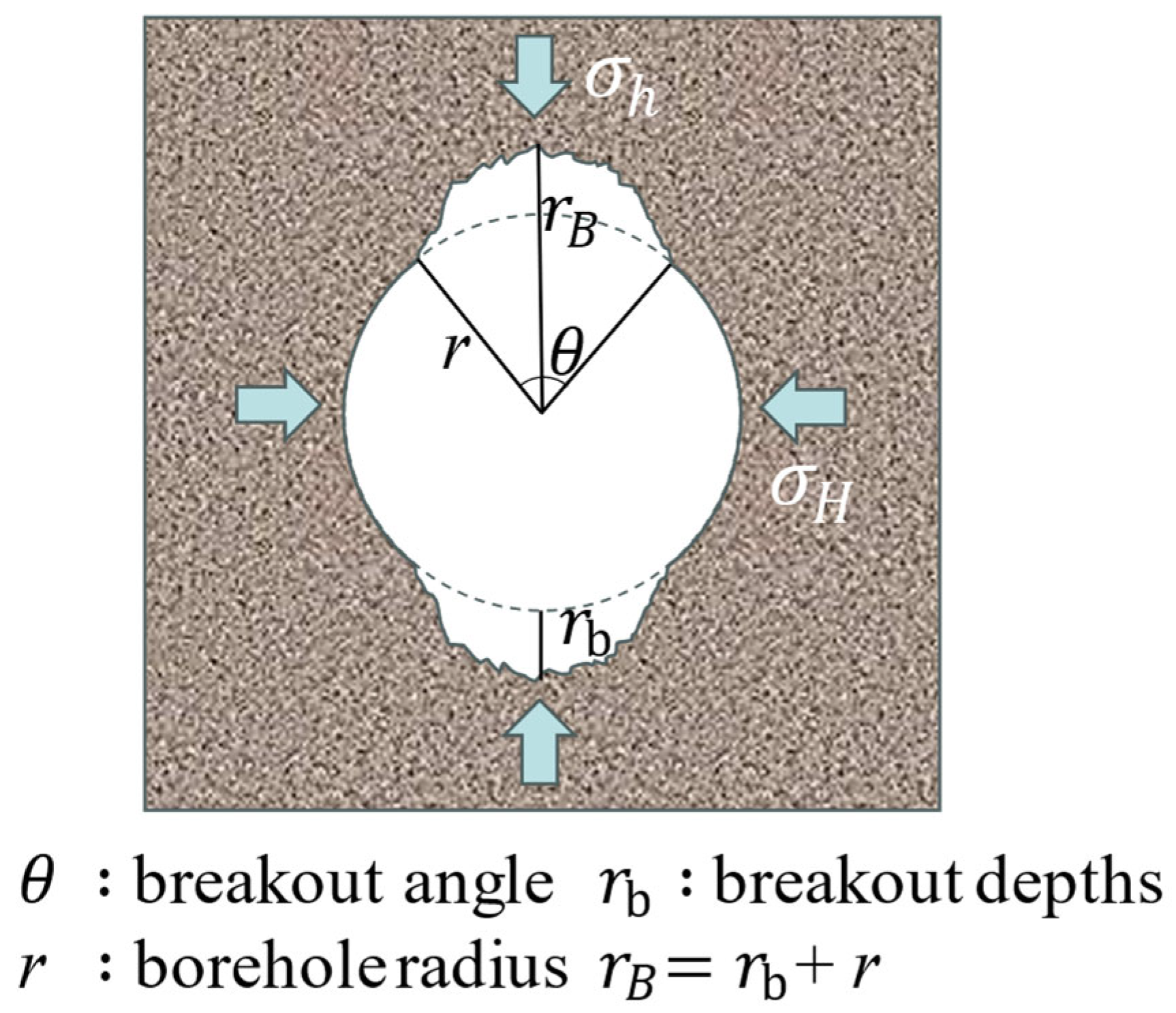
The borehole breakout phenomenon was first documented in a mining report from a South African gold mine [4] and later observed again in oil well development [5]. Further research revealed that in vertical boreholes, the direction of breakout consistently aligns parallel to the minimum horizontal in situ stress direction [6,7,8]. Meanwhile, the laboratory study identified the existence of two primary shapes of breakout, V-shape and dog-ear shape. Figure 1 illustrates the dog-ear-shaped borehole breakout shape with associated symbolic annotations. Significant disparities exist in the fracture mechanisms of rocks during the formation of the two breakout shapes, and their sizes demonstrate a notable correlation with the magnitude of in situ stresses [9]. Consequently, numerous researchers embarked on establishing the correlation between borehole breakout sizes and in situ stress, aiming to further elucidate the mechanism of borehole breakout. For example, Zoback et al. [10] combined the Mohr–Coulomb criterion with the Kirsch equation to develop a correlation model between in situ stress and borehole breakout size. Al-Ajmi [11] analyzed the vertical borehole stress distribution by linear elastic model and evaluated the rock stress state by Mogi–Coulomb criterion to construct the correlation between borehole mud pressure, borehole breakout and in situ stress.

However, because the process of borehole breakout is a continuous development, the stresses in the borehole wall and surrounding area will be further redistributed after the fractured rock is exfoliated, which will result in new rock exfoliation. Therefore, the models proposed by Zoback et al. [10] and Al-Ajmi [11] have certain limitations. The advancement of numerical simulation methods has offered an effective approach to addressing this issue, with several researchers successfully simulating the continuous development process of borehole breakout [12,13,14]. In recent years, numerous researchers have also been investigating borehole breakout through numerical simulation methods. For instance, in 2019, Lin et al. [15] examined the influence of borehole size and temperature on borehole breakout development using Discrete Element Method (DEM). They explored the pattern of microcrack development in the borehole wall and its surroundings under varying borehole sizes and temperatures. Zhang et al. [16] conducted a study on the impacts of borehole breakouts on breakdown pressure using finite element method (FEM) simulation. They established a correlation between in situ stress, borehole breakout size, and breakdown pressure. Xiang et al. [17] employed a three-dimensional bonded-particle model to simulate borehole breakout and successfully replicated the V-shape breakout phenomenon.

From the existing experimental, theoretical, and numerical simulation analyses and studies on borehole breakout, it is evident that the size of borehole breakout is influenced by factors such as mineral composition, porosity, grain strength, intergranular strength, angle of internal friction, cohesion, borehole mud pressure, temperature, in situ stress, Poisson’s ratio, rock modulus, and borehole size [18,19,20,21,22]. To achieve accurate assessment of borehole breakout, it is apparent that all relevant features should be considered as comprehensively as possible. The intricate nonlinear relationship among numerous features poses a significant challenge for conventional experimental and theoretical analyses, while numerical simulation is also complex and challenging. The emergence of machine learning (ML) methods offers a novel approach to address this issue.

Existing ML methods possess exceptional learning capabilities for capturing complex nonlinear relationships among different factors. Consequently, they have been widely applied by researchers for investigating engineering problems involving multi-feature considerations [23,24,25]. Furthermore, in Sharma et al.’s study, data from different wells were used to train the prediction model for the physical data of the rock at the drill bit during drilling, and the results had fairly good accuracy. This shows that machine learning models are well able to find potential nonlinear relationships between data from mixed datasets [26]. In the domain of borehole breakout assessment, ML methods have also seen extensive application. Table 1 collects some existing studies on ML for constructing borehole breakout association models, detailing the features, data sources, and algorithms they employed. The comparison reveals that the primary source of data for existing studies is finite element simulation. 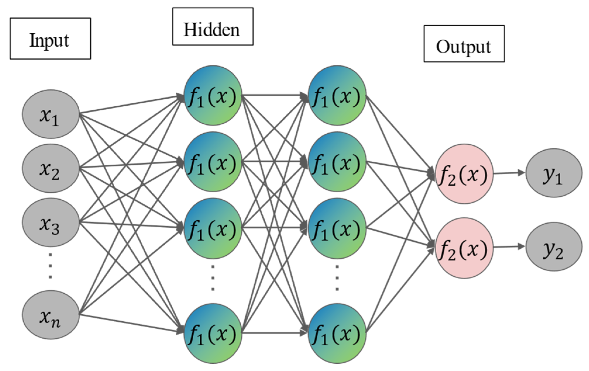Additionally, much of the data obtained through literature review also originates from FEM, as seen in the study by Benemaran [27]. It was observed that studies directly utilizing borehole breakout size as an output are categorized into single and multiple outputs, and multiple output studies mainly employ artificial neural network (ANN) [28,29,30].

Single output refers to constructing multiple models based on the same input features to predict multiple targets separately when dealing with problems involving multiple prediction targets. On the other hand, multi-output refers to constructing a single model to predict multiple targets simultaneously. Compared to single-output approaches, multi-output models take into account the relationship between input features and targets, while also considering potential interdependencies among targets and objectives [31,32]. Hence, when encountering multi-output problems with implicit relationships between outputs, multi-output models typically exhibit superior predictive performance compared to single-output models. Moreover, the training process of multi-output models tends to be more resource-efficient [33,34]. Existing studies lack theoretical research on the correlation between breakout angle and breakout depth. However, Soroush’s study demonstrates that incorporating breakout angle into input features significantly enhances the prediction accuracy of breakout depth. This indirectly suggests an implicit correlation between breakout angle and breakout depth [35]. Consequently, for predicting borehole breakout size, multi-output models hold considerable promise.

In existing multi-output studies on borehole breakout, single data sources are typically utilized, and certain crucial factors are often overlooked, resulting in limited generalization performance of the obtained models. Furthermore, no researcher has conducted a comparison between the established multi-output model and the single-output model, thus precluding the ability to ascertain the effectiveness of applying the multi-output structure. Obviously, further development and testing are still needed to validate the applicability of the multi-output structure in borehole breakout size prediction and to obtain models with high generalization performance and prediction accuracy for borehole breakout size prediction.

In this study, the prediction of borehole breakout size is treated as a multi-output problem considering the influence of multiple features. Through literature research, nine features deemed relevant to borehole breakout were selected as inputs to the model, and a dataset comprising 501 sets of related numerical simulation and physical experiment data was collected. To accurately map the potential connections between the input features and the target, a novel meta-heuristic optimization algorithm (WAOA) combined with three base models (ANN, RF, and XGBoost) was chosen to construct a hybrid multi-output model. The trained WAOA-ANN, WAOA-RF, and WAOA-XGBoost models were utilized to predict borehole breakout size under various conditions. Subsequently, the three hybrid multi-output models obtained are compared and discussed alongside the single-output model within the same setup to validate the effectiveness of employing the multi-output structure and to determine the optimal approach for borehole breakout size assessment. Finally, the relationship between the input features and outputs of the optimal models is analyzed and discussed using the SHAP sensitivity analysis method.

Table 1. Several borehole breakout prediction related studies.

Researchers	Data Source	Method	Input	Output	Best	Dataset	Output Form
Zhang et al. [29]	FEM	ANN	${\sigma }_h$ ${\sigma }_H$	$r_b$	R2: 0.99	training	Multi-output
				$\theta$
				$r_b$	R2: 0.99	validation
				$\theta$
				$r_b$	R2: 0.99	test
				$\theta$
Zhang et al. [28]	FEM	ANN	${\sigma }_h$ ${\sigma }_H$	$r_b$	R2: 0.99	training	Multi-output
				$\theta$
				$r_b$	R2: 0.99	validation
				$\theta$
				$r_b$	R2: 0.99	test
				$\theta$
Zhang and Yin [16]	FEM	ANN	${\sigma }_h$ ${\sigma }_H$	$r_b$	R2: 0.98	training	Multi-output
				$\theta$
				$r_b$	R2: 0.94	validation
				$\theta$
				$r_b$	R2: 0.99	test
				$\theta$
Lin, Singh et al. [36]	Literature Review, Laboratory experiment	ANN	${BWS}^{ 1}$ ${\sigma }_v$ $\theta$	${\sigma }_H$	R2: 0.74	training	Single-output
					R2: 0.95	validation
					R2: 0.82	test
Lin, Kang et al. [15]	Literature Review	Kriging	$BWS$ ${\sigma }_v$ $\frac{r_b}{r}$	${\sigma }_H$	MRE 2: 8.4%	test	Single-output
Soroush [35]	High quality acoustic image logs	MLPNN 8	${GR}^{ 3}$ ${RHOB}^{ 4}$${DTP}^{ 5}$${DTS}^{ 6}$${UCS}^{ 7}$ $\mu$ $\nu$	$\theta$	R2: 0.98	training	Multi-output
				$r_b$	R2: 0.65
				$\theta$	R2: 0.92	validation
				$r_b$	R2: 0.60
				$\theta$	R2: 0.94	test
				$r_b$	R2: 0.55
			$GR$ $RHOB$$DTP$$DTS$$UCS$ $\mu$ $\nu$ $\theta$	$r_b$	R2: 0.99	training	Single-output
					R2: 0.98	validation
					R2: 0.98	test
Jolfaei and Lakirouhani [37]	FEM	ANN	${\sigma }_h$ ${\sigma }_v$ ${\sigma }_H$ $\phi$ $c$	$\theta$	R2: 0.90	Total	Single-output
				$\frac{r_B}{r}$	R2: 0.85
Lin et al. [38]	Literature Review	ANN	$BWS$ ${\sigma }_v$ $\theta$	${\sigma }_h$	RMSE:3.29	training	Single-output
					RMSE:12.2	validation
		CART 9			RMSE:2.29	training
					RMSE:10.47	validation
Benemaran [27]	Literature Review	XGBoost	${\sigma }_h$ ${\sigma }_v$ ${\sigma }_H$ $\phi$ $c$	$\theta$	R2: 0.98	training	Single-output
					R2: 0.98	test
				$\frac{r_B}{r}$	R2: 0.99	training
					R2: 0.98	test
H. Zhang et al. [39]	Literature Review	SVR 10	$BWS$ $\theta$ $\frac{r_b}{r}$	${\sigma }_h$	MRE: 9.59%	test	Single-output

¹ $BWS$: borehole wall strength; ² MRE: mean relative error; ³ $GR$: gamma ray; ⁴ $RHOB$: formation bulk density; ⁵ $DTP$: compressional sonic; ⁶ $DTS$: shear sonic; ⁷ $UCS$: uniaxial compressive strength; ⁸ MLPNN: Multilayer Perceptron Neural Network; ⁹ CART: classification and regression tree; ¹⁰ SVR: support vector regressor.

Table 1. Several borehole breakout prediction related studies.

Researchers	Data Source	Method	Input	Output	Best	Dataset	Output Form
Zhang et al. [29]	FEM	ANN	${\sigma }_h$ ${\sigma }_H$	$r_b$	R2: 0.99	training	Multi-output
				$\theta$
				$r_b$	R2: 0.99	validation
				$\theta$
				$r_b$	R2: 0.99	test
				$\theta$
Zhang et al. [28]	FEM	ANN	${\sigma }_h$ ${\sigma }_H$	$r_b$	R2: 0.99	training	Multi-output
				$\theta$
				$r_b$	R2: 0.99	validation
				$\theta$
				$r_b$	R2: 0.99	test
				$\theta$
Zhang and Yin [16]	FEM	ANN	${\sigma }_h$ ${\sigma }_H$	$r_b$	R2: 0.98	training	Multi-output
				$\theta$
				$r_b$	R2: 0.94	validation
				$\theta$
				$r_b$	R2: 0.99	test
				$\theta$
Lin, Singh et al. [36]	Literature Review, Laboratory experiment	ANN	${BWS}^{ 1}$ ${\sigma }_v$ $\theta$	${\sigma }_H$	R2: 0.74	training	Single-output
					R2: 0.95	validation
					R2: 0.82	test
Lin, Kang et al. [15]	Literature Review	Kriging	$BWS$ ${\sigma }_v$ $\frac{r_b}{r}$	${\sigma }_H$	MRE 2: 8.4%	test	Single-output
Soroush [35]	High quality acoustic image logs	MLPNN 8	${GR}^{ 3}$ ${RHOB}^{ 4}$${DTP}^{ 5}$${DTS}^{ 6}$${UCS}^{ 7}$ $\mu$ $\nu$	$\theta$	R2: 0.98	training	Multi-output
				$r_b$	R2: 0.65
				$\theta$	R2: 0.92	validation
				$r_b$	R2: 0.60
				$\theta$	R2: 0.94	test
				$r_b$	R2: 0.55
			$GR$ $RHOB$$DTP$$DTS$$UCS$ $\mu$ $\nu$ $\theta$	$r_b$	R2: 0.99	training	Single-output
					R2: 0.98	validation
					R2: 0.98	test
Jolfaei and Lakirouhani [37]	FEM	ANN	${\sigma }_h$ ${\sigma }_v$ ${\sigma }_H$ $\phi$ $c$	$\theta$	R2: 0.90	Total	Single-output
				$\frac{r_B}{r}$	R2: 0.85
Lin et al. [38]	Literature Review	ANN	$BWS$ ${\sigma }_v$ $\theta$	${\sigma }_h$	RMSE:3.29	training	Single-output
					RMSE:12.2	validation
		CART 9			RMSE:2.29	training
					RMSE:10.47	validation
Benemaran [27]	Literature Review	XGBoost	${\sigma }_h$ ${\sigma }_v$ ${\sigma }_H$ $\phi$ $c$	$\theta$	R2: 0.98	training	Single-output
					R2: 0.98	test
				$\frac{r_B}{r}$	R2: 0.99	training
					R2: 0.98	test
H. Zhang et al. [39]	Literature Review	SVR 10	$BWS$ $\theta$ $\frac{r_b}{r}$	${\sigma }_h$	MRE: 9.59%	test	Single-output

¹ $BWS$: borehole wall strength; ² MRE: mean relative error; ³ $GR$: gamma ray; ⁴ $RHOB$: formation bulk density; ⁵ $DTP$: compressional sonic; ⁶ $DTS$: shear sonic; ⁷ $UCS$: uniaxial compressive strength; ⁸ MLPNN: Multilayer Perceptron Neural Network; ⁹ CART: classification and regression tree; ¹⁰ SVR: support vector regressor.

2. Methodologies

2.1. Artificial Neural Network (ANN)

Artificial neural network (ANN) are ML models that mimic the structure and function of biological neural networks, exhibiting strong learning capabilities for complex nonlinear problems [40,41]. Particularly suited for multiple-input multiple-output scenarios, ANN excels at learning and accurately mapping complex relationships between multi-input and multi-output variables. In the ANN model, the primary structure consists of an input layer, an output layer, and several hidden layers. Each layer comprises neurons, with the number of neurons in the input and output layers matching the number of input and output variables, respectively. There is no explicit requirement for the number of neurons per layer in the hidden layer. The input data are processed within neurons using a specific function called the activation function, and the results are then transmitted to neurons in the subsequent layer. The processing of input data by neurons can be represented by as:

$$y_j=f\left({\displaystyle \sum _{i=1}^n{w}_{ji}{x}_i+b_j}\right)$$

(1)

where $x_i$ is the $i$-th input data of the $j$-th neuron, $w_{ji}$ is the weight of the $i$-th input data of the $j$-th neuron, and $b_j$ is the bias of the $j$-th neuron. Figure 2 illustrates the fundamental structure of a multi-output ANN with two hidden layers.

2.2. Random Forest (RF)

Random forest (RF) belongs to the ensemble learning methods in ML algorithms, specifically categorized under the Bagging class. Its fundamental building block is the decision tree. The basic process for building a RF model involves: randomly selecting parts of training samples from the training set to create multiple new training sets; training multiple decision trees using the new training sets; aggregating the predictions of these decision trees to make the ultimate prediction. For regression tasks, the final output of RF model is the average of the predictions from the decision trees, while for classification tasks, it is the mode of the decision tree results. Figure 3 illustrates the algorithm flow of the RF model for regression prediction.

RF has been widely used in various fields such as medicine, biology, and engineering since it was proposed by Breiman in 1995 [42,43]. Compared to some existing ML algorithms, RF demonstrates higher accuracy and excellent performance in handling high-dimensional problems. Additionally, RF achieves good prediction accuracy even when dealing with missing values.

2.3. Extreme Gradient Boosting (XGBoost)

XGBoost is an ensemble learning algorithm that extends the gradient boosting decision tree algorithm by introducing regularization terms and second-order derivative information. It belongs to the Boosting class of ensemble algorithms and operates by integrating multiple weak learners into a single strong learner. The fundamental building block of XGBoost is the decision tree. Unlike random forest, in XGBoost, each subsequent decision tree is generated considering the residuals of the previous one, thereby continuously improving the learning of the model. Due to its exceptional learning and generalization capabilities, XGBoost has been successfully applied to numerous complex nonlinear problems. Moreover, XGBoost demonstrates strong applicability and outstanding accuracy in addressing multi-output problems [44].

2.4. The Walrus Optimization Algorithm (WAOA)

Trojovský and Dehghani propose a new meta-heuristic optimization algorithm called WAOA that mimics the behavior of walruses feeding, migrating, and avoiding predators in nature [45]. During each iteration of WAOA, the update of individual locations is divided into three phases: exploration, migration, and exploitation, as shown in Figure 4.

Phase 1 simulates the feeding behavior of walruses, in which walruses in the population move towards the leader which have optimal fitness for better feeding conditions. In this phase, the individual position update method can be expressed as:

$${X_i^p}^1(t+1)=X_i^3(t)+r_1(X_g-I_1{X}_i^3(t))$$

(2)

$$X_i^1\left(t+1\right)=\left\{\begin{array}{c}{X}_i^{p1}\left(t+1\right),f_i^{p1}<f_i\\ X_i\left(t\right),f_i^{p1}\ge f_i\end{array}\right.$$

(3)

where ${X_i^p}^1(t+1)$ denotes the new position of the $i$-th walrus obtained from the phase 1 update at iteration $t+1$, $X_i^3(t)$ denotes the $i$-th walrus position at iteration $t$, $r_1$ is a random number form the interval [0, 1], $X_g$ denotes the global best solution, $I_1$ is a random number form the interval [1, 2], $X_i^1(t+1)$ denotes the final position of $i$-th walrus obtained from the phase 1 update at iteration $t+1$, ${f_i^p}^1$ and $f_i$ denotes the fitness value while walrus’s position at ${X_i^p}^1(t+1)$ and $X_i\left(t\right)$ respectively.

Phase 2 simulates the migration behavior of walruses. During the migration process, the walrus moves toward to a random select walrus, which can represent use:

$$X_i^{p2}\left(t+1\right)=\left\{\begin{array}{c}{X}_i^1(t+1)+r_2(X_r^1(t+1)-I_2{X}_i^1(t+1)),f_r<f_i^1\\ X_i^1(t+1)+r_2(X_i^1(t+1)-X_r^1(t+1)),f_r\ge f_i^1\end{array}\right.$$

(4)

$$X_i^2\left(t+1\right)=\left\{\begin{array}{c}{X}_i^{p2}\left(t+1\right),f_i^{p2}<{f_i^p}^1\\ X_i^1\left(t+1\right),f_i^{p2}\ge {f_i^p}^1\end{array}\right.$$

(5)

where ${X_i^p}^2(t+1)$ denotes the new position of the $i$-th walrus obtained from the phase 2 update at iteration $t+1$, $X_r^1\left(t+1\right)$ denotes the position of selected walrus that the $i$-th walrus toward to migrate and $f_r$ denotes its fitness value, $f_i^1$ denotes the fitness value while walrus’s position at $X_i^1(t+1)$, $X_i^2(t+1)$ denotes the final position of $i$-th walrus obtained from the phase 2 update at iteration $t+1$, $r_2$ and $I_2$ are random number taken from the intervals [0, 1] and [1, 2], respectively, $f_i^{p2}$ denotes the fitness value while walrus’s position at ${X_i^p}^2(t+1)$.

Phase 3 simulates the natural behavior of walruses escaping and fighting with the predators, which can represent use:

$${X_i^p}^3(t+1)=X_i^2(t+1)+(L{B}_{(t+1)}+(U{B}_{(t+1)}-r_{3}L{B}_{(t+1)}))$$

(6)

$$\left\{\begin{array}{c}L{B}_{t+1}=\frac{LB}{t+1}\\ U{B}_{t+1}=\frac{UB}{t+1}\end{array}\right.$$

(7)

$$X_i^3\left(t+1\right)=\left\{\begin{array}{c}{X}_i^{p3}\left(t+1\right),f_i^{p3}<f_i^2\\ X_i^2\left(t+1\right),f_i^{p3}\ge f_i^2\end{array}\right.$$

(8)

where ${X_i^p}^3(t+1)$ denotes the new position of the $i$-th walrus obtained from the phase 3 update at iteration $t+1$, $r_3$ is a random number form the interval [0, 1], $X_i^3(t+1)$ denotes the final position of $i$-th walrus obtained from the phase 3 update at iteration $t+1$, $LB$ and $UB$ denotes the lower and upper bounds of the walrus’s position, respectively, $f_i^2$ denotes the fitness value while walrus’s position at $X_i^2(t+1)$, $f_i^{p3}$ denotes the fitness value while walrus’s position at ${X_i^p}^3(t+1)$.

3. Data Description and Evaluation Metrics

Existing research on borehole breakout can be categorized into numerical simulation and physical experiments in terms of experimental methods. Numerical simulation offers greater convenience in setting up various external conditions to explore the influence of multiple dimensions, making it favored by many scholars. However, the results of physical experiments exhibit better consistency with field reality. In this paper, data obtained from both methods are considered. It is important to note that only data from FEM simulations were collected, as most Discrete Element Method (DEM) simulations were two-dimensional and did not account for the effect of vertical in situ stress [1,15,46].

Through literature research [19,20,22,27,35], the following input features were selected from a wide range of features associated with borehole breakout: rock internal friction angle ($\phi$), cohesion ($c$), rock modulus ($E$), Poisson’s ratio ($\nu$), mud pressure in the borehole ($P_w$), minimum horizontal principal stress (${\sigma }_h$), vertical principal stress (${\sigma }_v$), maximum horizontal principal stress (${\sigma }_H$), and the radius of the borehole ($r$).

Meanwhile, a total of 501 sets of relevant data were collected from the existing research literature to construct a borehole breakout size dataset [16,28,29,30,37,47,48,49,50,51]. Considering that the absolute magnitude of the borehole breakthrough depth is significantly correlated with the borehole radius, and that the borehole radius setting varies in different studies, the borehole breakthrough depth is dimensionless normalized to improve the model generalization ability.

Table 2. Statistical description of features in the datasets.

Variables	Unit	FEM			Experiment
		Min	Max	Mean	Min	Max	Mean
$\theta$	°	0	81	45.82	25	138	68.04
$\frac{r_b}{r}$		0	2.19	0.49	0.02	1.53	0.52
$r$	cm	10	15	13.61	0.8	1.5	1.1
${\sigma }_H$	MPa	50	200	103.19	35.4	93.2	61.74
${\sigma }_v$	MPa	30	80	47.83	5	50	31.67
${\sigma }_h$	MPa	20	85	48.61	10	40	23.54
$P_w$	MPa	0	45	19.03	0	0	0
$\nu$		0.2	0.25	0.21	0.17	0.27	0.22
$E$	GPa	14.4	59	26.83	6.66	27	15.12
$c$	MPa	6	55	18.66	8.92	15.5	11.83
$\phi$	°	32.5	52.5	39.13	18	39.7	31.54

summarizes the statistical metrics of the constructed dataset, taking into account the significant variation in borehole sizes involved in different studies, and transforming the borehole breakout depths accordingly. Additionally, it is noted that in the physical experiments, none of them set the mud pressure in the borehole, thus it is considered to be 0 MPa.

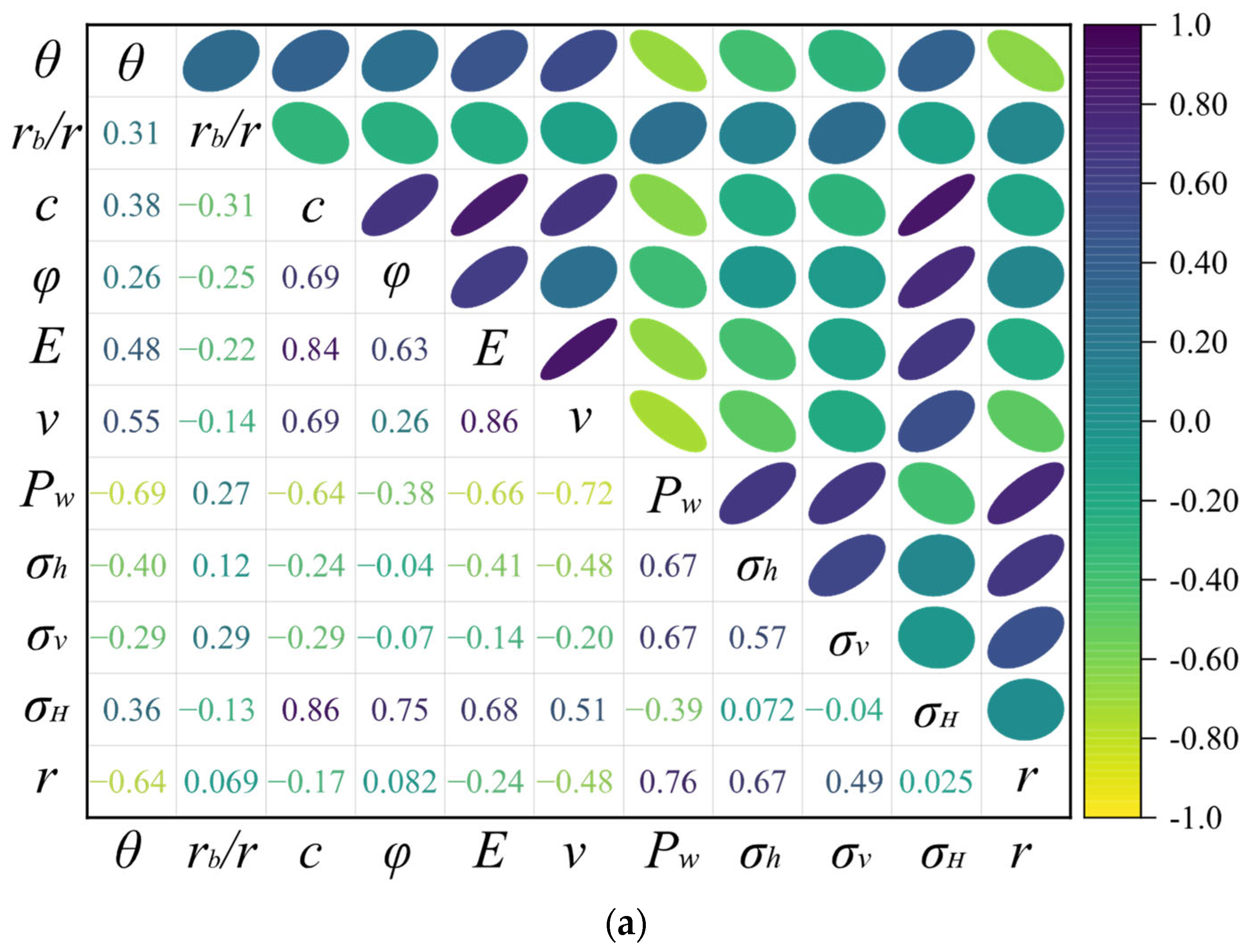
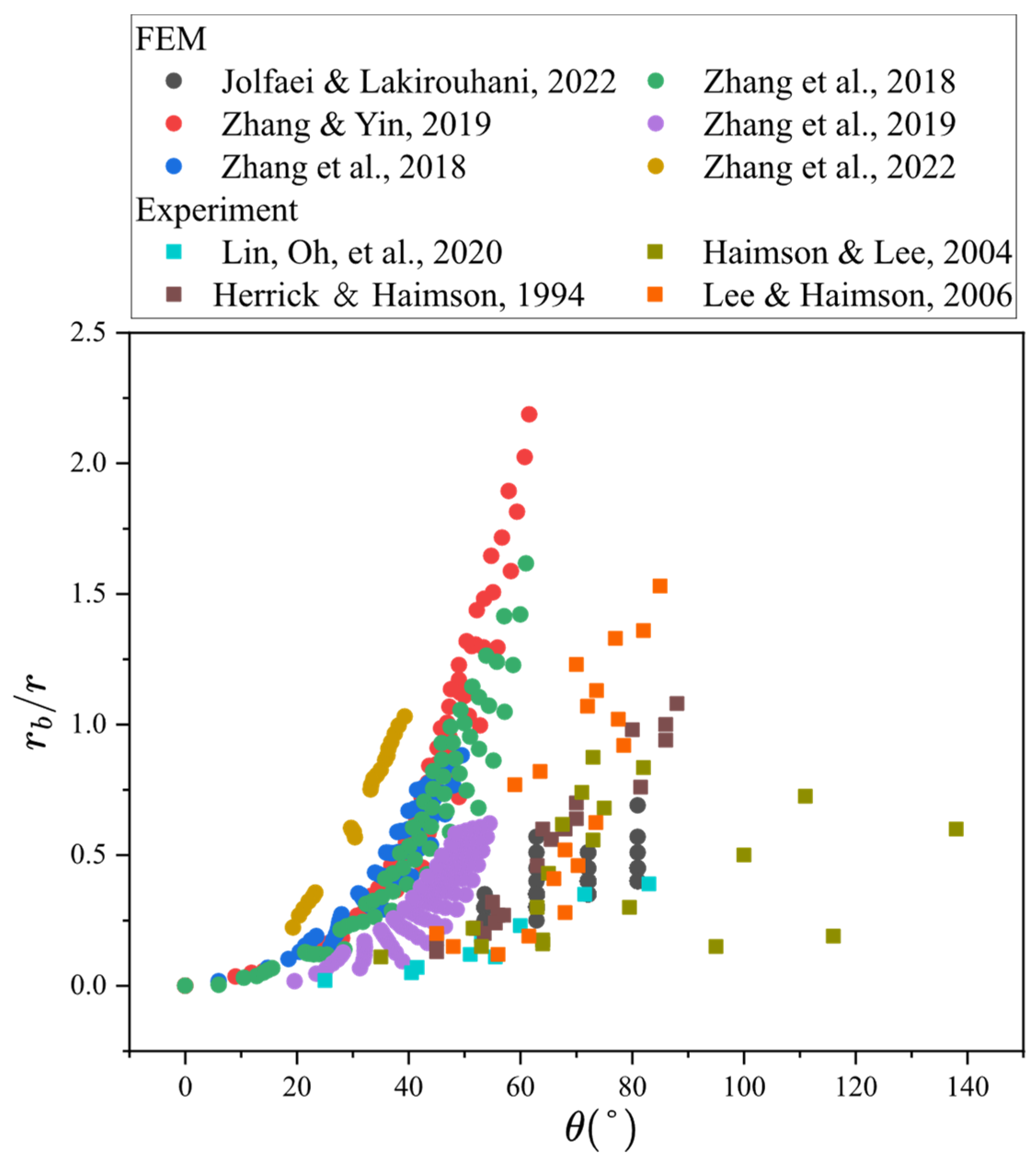
Figure 5 illustrates the distribution relationship between the breakout sizes. From the figure, it is evident that all the borehole breakout sizes obtained by different researchers exhibit a pronounced nonlinear relationship. This initial observation confirms the feasibility of employing the multi-output approach for borehole breakout size prediction. Additionally, the correlation analysis between the input features and borehole breakout size is further presented in Figure 6.

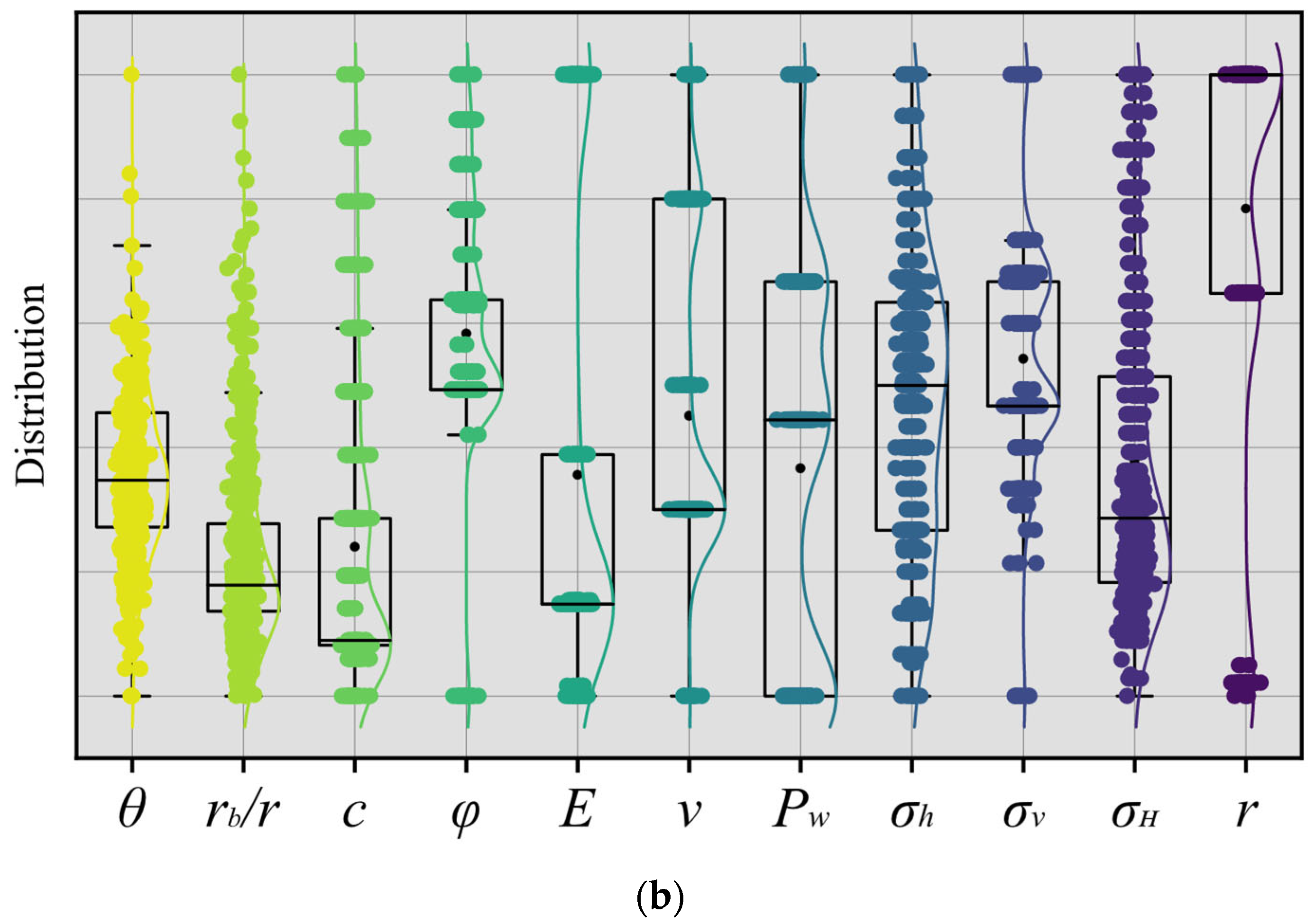
The correlation analysis of the dataset aims to assess whether there is excessive correlation among the input features, potentially leading to multicollinearity issues that could impact the model’s performance. As illustrated in Figure 6a, the highest correlation observed between features is 0.86. Notably, for identical input features, the borehole breakout angle and depth exhibit completely opposite correlations. Additionally, an input-output distribution analysis is conducted to identify and mitigate the presence of outliers in the dataset, which could disrupt model training and evaluation. Figure 6b illustrates that there are no apparent outliers in the dataset. Furthermore, it is evident that the distribution of features $c,\phi ,{\sigma }_h,{\sigma }_v,{\sigma }_H$ is more uniform, whereas the distribution of features $E,\nu ,P_w,r$ is denser. Consequently, the primary focus of the study appears to be on features $c,\phi ,{\sigma }_h,{\sigma }_v,{\sigma }_H$.

Reasonably setting evaluation metrics for model assessment is crucial for selecting the optimal model correctly. Drawing from previous ML studies [52,53,54,55,56,57,58,59,60], commonly used evaluation metrics include the Pearson Correlation Coefficient (R²), Mean Absolute Error (MAE), Variance Accounted For (VAF), and Root Mean Squared Error (RMSE). The calculation methods for these metrics are outlined as:

$$R^2=\frac{{\left[{\displaystyle \sum _{i=1}^n(f_i-\overline{f})(y_i-\overline{y})}\right]}^2}{{\displaystyle \sum _{i=1}^n{(f_i-\overline{f})}^2{\displaystyle \sum _{i=1}^n{(y_i-\overline{y})}^2}}}$$

(9)

$$MAE=\frac{1}{n}{\displaystyle \sum _{i=1}^n\left|f_i-y_i\right|}$$

(10)

$$VAF=1-\frac{\mathrm{var}(f_i-y_i)}{\mathrm{var}(y_i)}$$

(11)

$$RMSE=\sqrt{\frac{{\displaystyle \sum _{i=1}^n{(f_i-y_i)}^2}}{n}}$$

(12)

where $f$ denotes the predicted value, $\overline{f}$ denotes the mean of the predicted values, $y_i$ denotes the actual value, $\overline{y}$ denotes the mean of the actual values, $n$ denotes the number of data.

4. Result and Discussion

4.1. Model Training

In this study, a novel meta-heuristic optimization algorithm, WAOA, is combined with ANN, RF, and XGBoost to construct more efficient hybrid multi-output models for predicting borehole breakout size. According to the experience and theoretical research of researchers on hyperparameter adjustment of ANN, RF and XGBoost regression prediction model with multi-feature input, the hyperparameter objects and ranges optimized by WAOA in this study are shown in

Table 3. Hyperparameter settings and optimization ranges.

Method	Hyperparameters	Range	Parameter Meaning
ANN	Learning rate	[0.00001, 0.1]	Learning rate of the optimizer
	Num dense layers	[1, 10]	Number of hidden layers
	Num dense nodes	[5, 110]	Number of nodes for each layer
	Activation	Relu	Activation function
RF	n_estimators	[1, 1100]	The number of trees
	max_depth	[10, 1100]	The maximum tree depth
XGBoost	max_depth	[1, 10]	The maximum tree depth
	learning_rate	(0, 1]	Rate of iteration
	n_estimators	[1, 500]	The number of trees

.

Figure 7 illustrates the construction, optimization and comparison process of the hybrid multi-output model proposed in this study. After determining the influencing factors of borehole breakout size by analyzing and comparing the existing literature, a substantial amount of relevant data was collected from the existing literature to construct a dataset. To balance the accuracy requirement of the model to explore the intricate nonlinear relationship between input and output factors in the training process, and the rigor requirement of the model comparison process, the dataset was randomly divided into the training set (80%) and the test set (20%).

To comprehensively investigate the intricate nonlinear relationship between input features and borehole breakout size, and to leverage the potential correlation between breakout size, the ANN, RF, and XGBoost was employed as the foundation, with WAOA utilized as the optimization tool to develop a hybrid multi-output prediction model for borehole breakout size. In the optimization process of WAOA, MSE is chosen as the fitness evaluation metric which can be calculated as:

$$MSE=\frac{{\displaystyle \sum _{i=1}^n{(f_i-y_i)}^2}}{n}$$

(13)

Simultaneously, to address inconsistencies in units among different outputs and ensure a balanced consideration of various output prediction accuracies in the overall fitness evaluation of the model, all input and output features were normalized to [0, 1]. The normalization process can be presented as:

$$x=\frac{x^{\prime }-x_{\min }}{x_{\max }-x_{\min }}$$

(14)

where $x$ denotes the value after normalization, $x^{\prime }$ denotes the value before normalization, $x_{\min }$ denotes the minimum value of the feature, $x_{\max }$ denotes the maximum value of the feature. This normalization is an equiproportional transformation of the entire range of features, it does not change the distribution shape of the features, and therefore does not disrupt the potential nonlinear relationships in the dataset.

Since model hyperparameter optimization involves continuously adjusting the hyperparameter settings to fit the training data, overfitting is prone to occur if a single training set is used exclusively for training and evaluating the fitness of adjustments. To mitigate the risk of overfitting in the iterative process of the hybrid multi-output model, 5-fold cross-validation was employed during model training. Multifold cross-validation is an effective method for preventing overfitting during iteration and enhancing model generalization performance. By iteratively dividing the training set data into training and testing folds, multiple validations of the model’s performance for a given hyperparameter setting were conducted to accurately assess the effectiveness of hyperparameter adjustments.

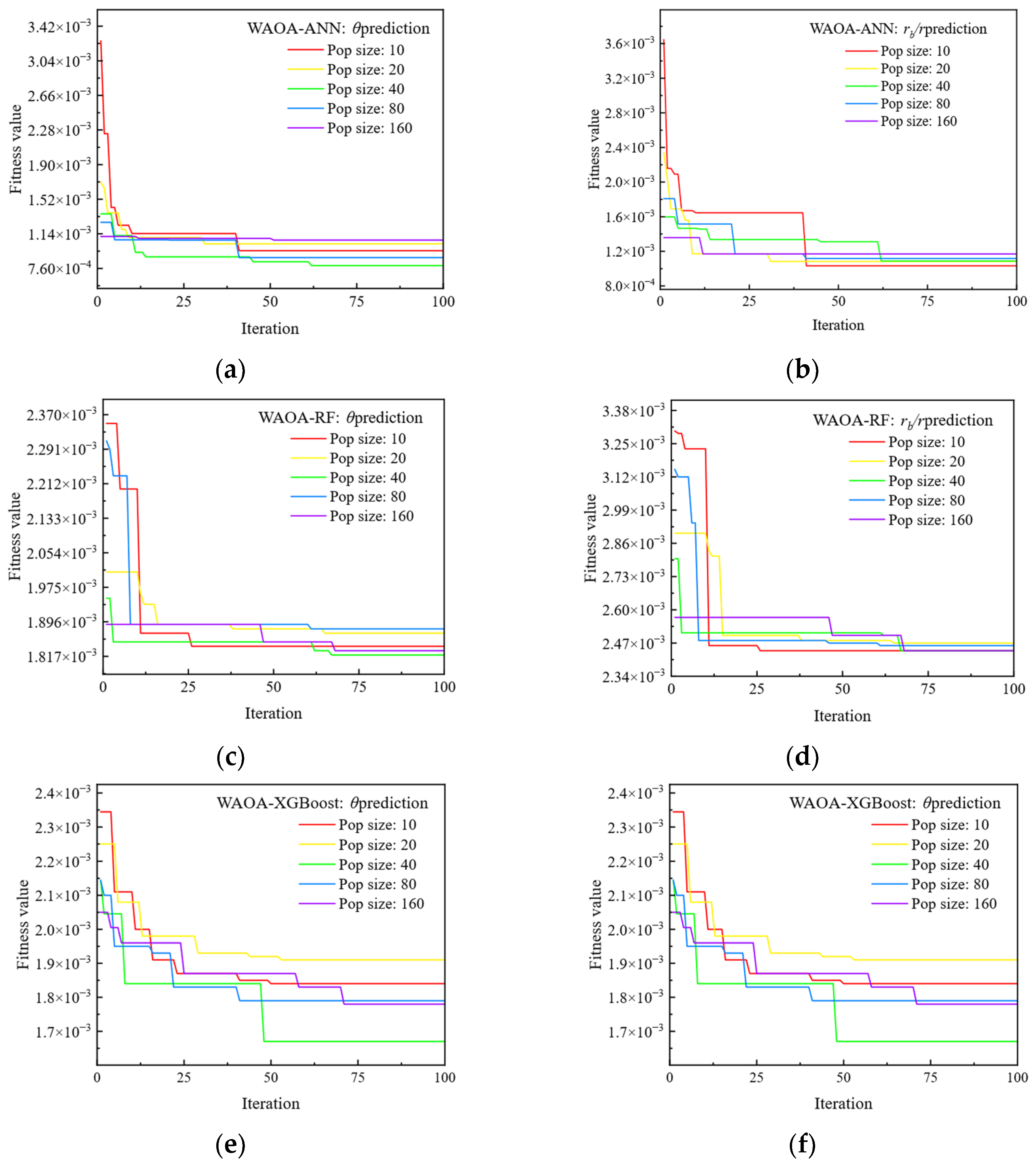
Drawing from previous research experience, the optimization effect of the meta-heuristic optimization algorithm on the target model is significantly influenced by the population size. Therefore, in this study, five different population sizes (10, 20, 40, 80, 160) will be employed to enable the optimization algorithm to accurately search for high-performance hyperparameter settings. Figure 8 illustrates the curve of model fitness with the number of iterations for different population size settings, and it can be seen that the fitness of the model stabilizes as the number of iterations increases. The ultimate hyperparameter settings of the model through the optimization of WAOA at different population size settings are shown in

Table 4. Optimal parameters obtained by WAOA for different Models.

Model	Hyperparameters	Pop Size
		10	20	40	80	160
WAOA-ANN	Learning rate	$4.8307\times {10}^{-4}$	$5.4203\times {10}^{-4}$	$3.2513\times {10}^{-4}$	$8.0645\times {10}^{-4}$	$7.0801\times {10}^{-4}$
	Num dense layers	4	5	6	3	1
	Num dense nodes	100	83	51	89	82
WAOA-RF	n_estimators	274	478	95	1000	93
	max_depth	510	273	48	1000	949
WAOA-XGBoost	max_depth	3	4	4	4	4
	n_estimators	500	444	500	374	239
	learning_rate	0.3412	0.2143	0.2275	0.1626	0.4481

.

Table 5. Evaluation metrics performance of different WAOA-ANN models.

Pop Size	Training
	R2 (Score)		MAE (Score)		VAF (Score)		RMSE (Score)
	$\mathit{\theta }$	${\mathit{r}}_{\mathit{b}}/\mathit{r}$	$\mathit{\theta }$	${\mathit{r}}_{\mathit{b}}/\mathit{r}$	$\mathit{\theta }$	${\mathit{r}}_{\mathit{b}}/\mathit{r}$	$\mathit{\theta }$	${\mathit{r}}_{\mathit{b}}/\mathit{r}$
10	0.9906(5)	0.9839(4)	0.0095(5)	0.0167(5)	0.9803(5)	0.9679(4)	0.018(5)	0.0284(4)
20	0.9885(4)	0.9825(2)	0.0107(4)	0.0168(3)	0.9766(4)	0.9645(2)	0.0195(4)	0.0298(2)
40	0.9867(2)	0.9828(3)	0.0127(2)	0.0175(2)	0.9726(2)	0.9651(3)	0.0212(2)	0.0296(3)
80	0.9874(3)	0.9847(5)	0.0113(3)	0.0167(4)	0.9742(3)	0.969(5)	0.0205(3)	0.0279(5)
160	0.9834(1)	0.9809(1)	0.0132(1)	0.0183(1)	0.9662(1)	0.9613(1)	0.0235(1)	0.0312(1)
	Test
	R2 (score)		MAE (score)		VAF (score)		RMSE (score)
	$\theta$	$r_b/r$	$\theta$	$r_b/r$	$\theta$	$r_b/r$	$\theta$	$r_b/r$
10	0.9819(5)	0.978(2)	0.0142(5)	0.0208(3)	0.9629(5)	0.9556(2)	0.0244(5)	0.0334(2)
20	0.9813(4)	0.9758(1)	0.0157(3)	0.0212(2)	0.9628(4)	0.9511(1)	0.0244(4)	0.035(1)
40	0.9791(2)	0.9803(5)	0.0166(2)	0.0187(5)	0.9572(2)	0.9601(5)	0.0262(2)	0.0316(5)
80	0.9804(3)	0.9784(3)	0.0153(4)	0.0203(4)	0.9601(3)	0.9567(3)	0.0253(3)	0.033(3)
160	0.9742(1)	0.9787(4)	0.0168(1)	0.022(1)	0.9489(1)	0.9574(4)	0.0286(1)	0.0327(4)

,

Table 6. Evaluation metrics performance of different WAOA-RF models.

Pop Size	Training
	R2 (Score)		MAE (Score)		VAF (Score)		RMSE (Score)
	$\mathit{\theta }$	${\mathit{r}}_{\mathit{b}}/\mathit{r}$	$\mathit{\theta }$	${\mathit{r}}_{\mathit{b}}/\mathit{r}$	$\mathit{\theta }$	${\mathit{r}}_{\mathit{b}}/\mathit{r}$	$\mathit{\theta }$	${\mathit{r}}_{\mathit{b}}/\mathit{r}$
10	0.9936(4)	0.9943(1)	0.0084(3)	0.0096(1)	0.9862(4)	0.9877(1)	0.015(4)	0.0176(1)
20	0.9934(3)	0.9948(5)	0.0083(4)	0.0093(5)	0.9857(3)	0.9885(5)	0.0153(3)	0.017(5)
40	0.9932(2)	0.9947(4)	0.0085(2)	0.0095(2)	0.9852(2)	0.9884(4)	0.0155(2)	0.0171(4)
80	0.9938(5)	0.9946(3)	0.0083(5)	0.0093(4)	0.9864(5)	0.9881(3)	0.0149(5)	0.0173(3)
160	0.9929(1)	0.9944(2)	0.0086(1)	0.0094(3)	0.9848(1)	0.9879(2)	0.0158(1)	0.0174(2)
	Test
	R2 (score)		MAE (score)		VAF (score)		RMSE (score)
	$\theta$	$r_b/r$	$\theta$	$r_b/r$	$\theta$	$r_b/r$	$\theta$	$r_b/r$
10	0.9699(4)	0.9642(1)	0.018(3)	0.0226(1)	0.9382(4)	0.9195(1)	0.0314(4)	0.0449(1)
20	0.9689(3)	0.9661(5)	0.0177(4)	0.0218(5)	0.9367(3)	0.9223(4)	0.0318(3)	0.0441(4)
40	0.968(1)	0.9651(2)	0.0184(1)	0.0224(2)	0.9349(1)	0.9201(2)	0.0323(1)	0.0448(2)
80	0.9704(5)	0.9657(3)	0.0174(5)	0.0218(4)	0.9395(5)	0.9219(3)	0.0311(5)	0.0443(3)
160	0.9685(2)	0.966(4)	0.0181(2)	0.0221(3)	0.9358(2)	0.9237(5)	0.0321(2)	0.0438(5)

and

Table 7. Evaluation metrics performance of different WAOA-XGBoost models.

Pop Size	Training
	R2 (Score)		MAE (Score)		VAF (Score)		RMSE (Score)
	$\mathit{\theta }$	${\mathit{r}}_{\mathit{b}}/\mathit{r}$	$\mathit{\theta }$	${\mathit{r}}_{\mathit{b}}/\mathit{r}$	$\mathit{\theta }$	${\mathit{r}}_{\mathit{b}}/\mathit{r}$	$\mathit{\theta }$	${\mathit{r}}_{\mathit{b}}/\mathit{r}$
10	0.9999(5)	0.9999(5)	0.0009(5)	0.0008(5)	0.9999(5)	0.9999(5)	0.0013(5)	0.0019(5)
20	0.9995(1)	0.9996(2)	0.0027(1)	0.0029(2)	0.999(1)	0.9992(2)	0.004(1)	0.0044(2)
40	0.9997(3)	0.9996(1)	0.0023(4)	0.003(1)	0.9993(3)	0.9992(1)	0.0033(3)	0.0045(1)
80	0.9995(2)	0.9996(3)	0.0026(2)	0.0029(3)	0.9991(2)	0.9992(3)	0.0039(2)	0.0044(3)
160	0.9997(4)	0.9997(4)	0.0023(3)	0.0025(4)	0.9993(4)	0.9995(4)	0.0033(4)	0.0037(4)
	Test
	R2 (score)		MAE (score)		VAF (score)		RMSE (score)
	$\theta$	$r_b/r$	$\theta$	$r_b/r$	$\theta$	$r_b/r$	$\theta$	$r_b/r$
10	0.9392(1)	0.96(1)	0.0261(1)	0.0262(1)	0.8819(1)	0.9194(1)	0.0435(1)	0.045(1)
20	0.976(3)	0.9816(5)	0.0157(3)	0.0164(5)	0.9524(3)	0.9628(5)	0.0276(3)	0.0305(5)
40	0.9796(5)	0.9748(2)	0.0151(4)	0.0187(3)	0.9594(5)	0.949(2)	0.0255(5)	0.0358(2)
80	0.9776(4)	0.9789(4)	0.0149(5)	0.0172(4)	0.9555(4)	0.9573(4)	0.0267(4)	0.0327(4)
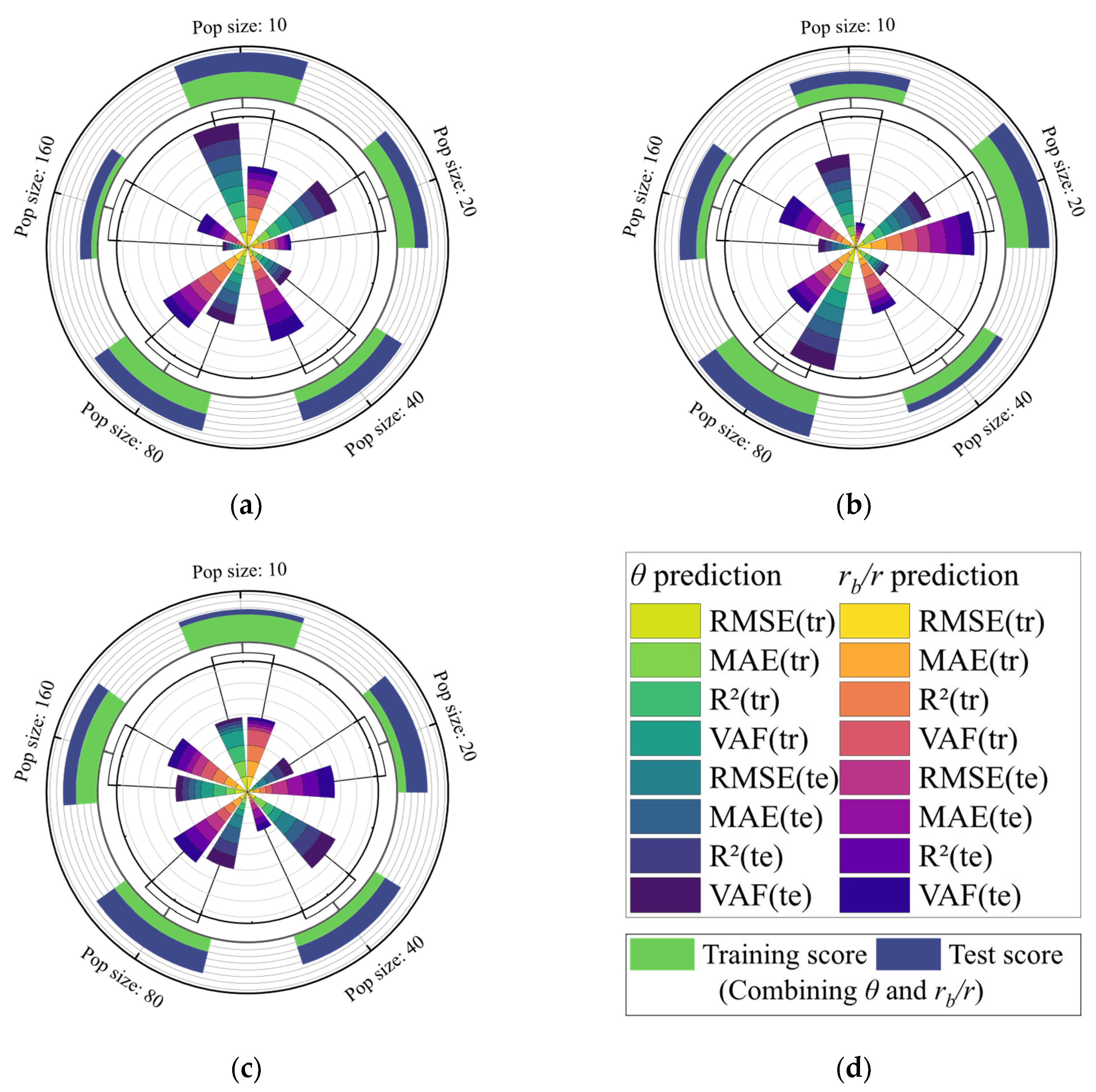
160	0.973(2)	0.9756(3)	0.016(2)	0.0195(2)	0.9462(2)	0.9501(3)	0.0293(2)	0.0354(3)

summarize the performance and ranking scores of the models trained under different pop sizes on the four predictive evaluation metrics used, and Figure 9 provides a visual comparison of the model performance scores. Figure 9 combines the rank of the models on various indicators and assigns scores to them, enabling a comprehensive comparison of multiple indicators with different scales. In the subplots of Figure 9, the internal wind rose plot represents the model’s separate scores for predicting $\theta$ and $r_b/r$, and the external one represents the model’s combined scores for predicting $\theta$ and $r_b/r$ on the training and test sets.

4.1.1. Determination of Optimal WAOA-ANN Models

In multi-output ANN models, different outputs share the output layer and the hidden layer, and thus the adjustment of the weights and biases of the hidden layer neurons during the training process is jointly affected by all outputs. The differences between different outputs are mainly caused by the differences in the weights and biases adopted by their respective output layer neurons. The fitness curves of the five WAOA-ANN models under different pop sizes are shown in Figure 8a,b. From the figure, for the prediction of $\theta$, the optimal fitness of the model is stable between $7.06\times {10}^{-4}$ and $1.14\times {10}^{-3}$, while for the prediction of $r_b/r$, the optimal fitness of the model is stable between $8\times {10}^{-4}$ and $1.2\times {10}^{-3}$. There is a significant decrease in fitness compared to when iterating the initial model.

Even though the model fitness is evaluated by 5-fold cross-validation during the iteration process, overfitting of the model is largely avoided. However, during each iteration, the data in the training set are directly or indirectly involved in the assessment of model fitness, and because it is a multi-output model, the model may not perform equally on two predicted objects, so the ranking of the final model fitness cannot completely reflect the model prediction performance. To completely evaluate the model prediction performance and generalization performance to select the optimal WAOA-ANN model, the resulting models are further compared on the training and test sets. Table 5 lists the prediction performance and ranking scores of the five WAOA-RF models on the training and test sets. As can be seen from Table 5, there is no model that can rank first in both $\theta$ and $r_b/r$ prediction on both the training and test sets at the same time. For example, the WAOA-RF model obtained with a pop size setting of 10 ranks first in all four metrics for the prediction of $\theta$ on the training set and test set, but ranks poorly for the prediction of $r_b/r$ on test set. This suggests that multi-output ANN models with different hyperparameter settings have their own focus on different outputs. For the sake of model comprehensiveness, a superior multi-output model should be balanced in the prediction performance of different outputs. Therefore, further the predictive performance of different WAOA-ANN models for $\theta$ and $r_b/r$ on the training set and the test set is shown in Figure 9a. As can be seen in Figure 9a, for the five WAOA-ANN models obtained, the models with the pop size setting of 10 and 80 accounted for the highest scores for $\theta$ and $r_b/r$ predictions, respectively, and the model with a pop size of 10 (Num dense layers = 4, Num dense nodes = 100, Learning rate = $4.8307\times {10}^{-4}$) had the highest combined score. Therefore, in the subsequent study, the WAOA-ANN model with a pop size of 10 was used as a representative of the WAOA-ANN model.

4.1.2. Determination of Optimal WAOA-RF Models

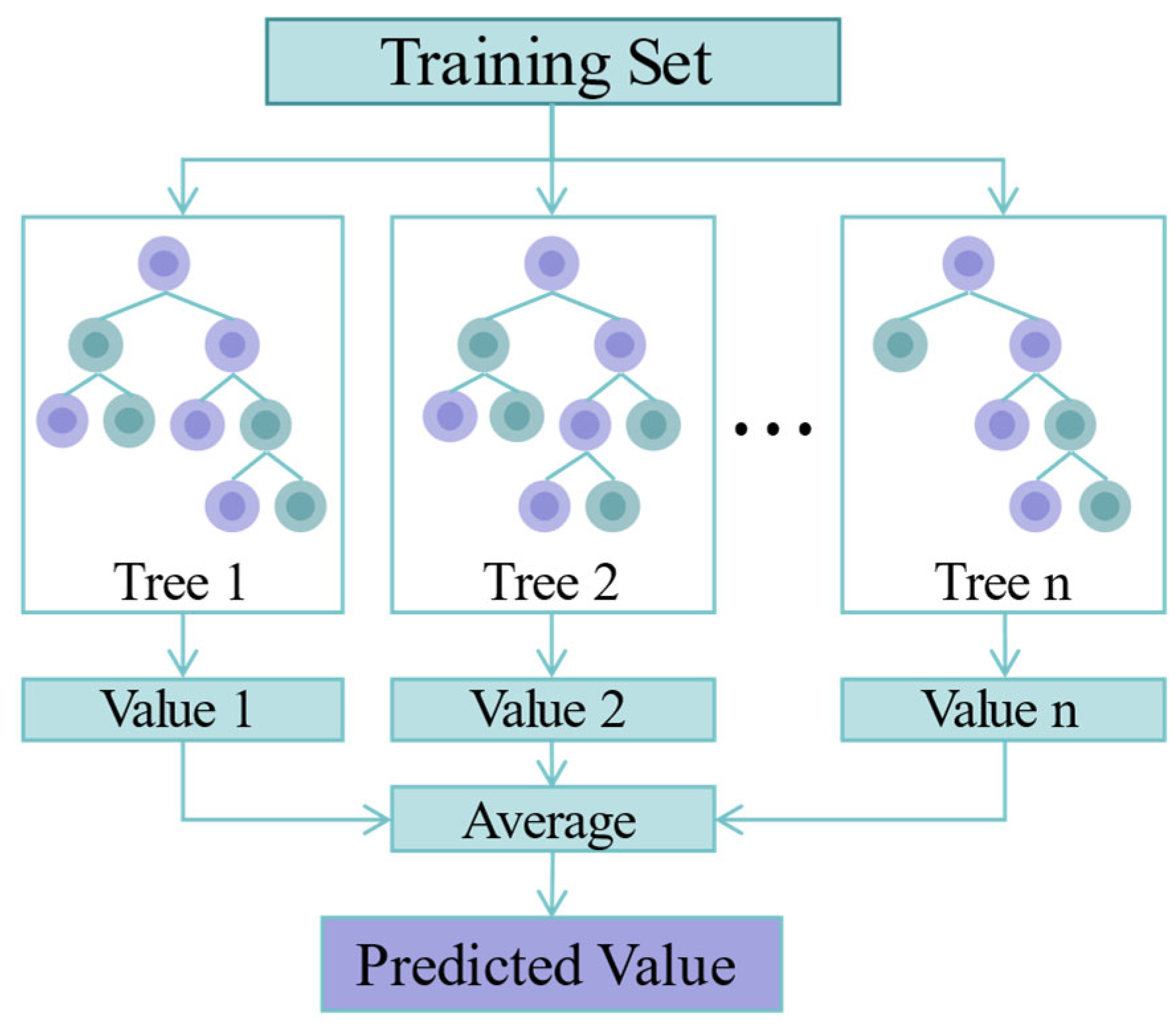
For multi-output RF models, node splitting takes into account the variance of the different outputs in the child nodes when constructing the decision tree to achieve a comprehensive consideration of the different outputs. Figure 8c,d illustrate the variation in fitness during iterations of the WAOA-RF model. As can be seen from the figure, the distribution of the optimal fitness of the five WAOA-RF models for the prediction of $\theta$ ranges from $1.817\times {10}^{-3}$ and $1.863\times {10}^{-3}$, and the distribution of the prediction of $r_b/r$ ranges from $2.34\times {10}^{-3}$ and $2.47\times {10}^{-3}$. Table 6 shows the performance of the five WAOA -RF models in terms of evaluation metrics on the training and test sets, as well as their ranking scores. From Table 6, it can be noticed that the model with a pop size of 80 takes the absolute lead in the performance of the training set and test set, in the prediction of θ (training set: R² = 0.9938, MAE = 0.0083, VAF = 0.9864, RMSE = 0.0149, test set: R² = 0. 9704, MAE = 0.0174, VAF = 0. 9395, RMSE = 0.0311). Further analyses of Figure 9b revealed that the models with pop size 80 and 20 occupy the highest scores for predicting $\theta$ and $r_b/r$, respectively, and the model with the highest combined score is the model with pop size 80 (n_estimators = 1000, max_depth = 1000).

4.1.3. Determination of Optimal WAOA-XGBoost Models

The multi-output XGBoost model has the same node splitting strategy as the multi-output RF model when constructing decision trees. The difference is that XGBoost takes into account the bias of the previous decision tree when constructing a new decision tree, effectively reducing the variation in prediction performance between different outputs. From Figure 8e,f, the optimal fitness of the five WAOA-XGBoost models is distributed between $1.6\times {10}^{-3}$ and $2.0\times {10}^{-3}$ for the prediction of $\theta$, and between $1.7\times {10}^{-3}$ and $2.5\times {10}^{-3}$ for the prediction of $r_b/r$. Table 7 summarizes the prediction performance and ranking scores of the five WAOA-XGBoost models on the training and test sets. As can be seen from the table, the prediction performance and ranking scores of most WAOA-XGBoost models in $\theta$ and $r_b/r$ are relatively consistent. This can be observed more intuitively in Figure 9c, where the models with pop sizes of 10, 80 and 160 each have essentially the same scores on $\theta$ and $r_b/r$. This confirms the balanced consideration of potential links between different outputs and input features in the multi-output XGBoost model.

It can also be seen from Figure 9c that the model with a pop size of 10 occupies the highest score for predicting $\theta$. The model with a pop size of 80 (max_depth = 4, n_estimators = 374, learning_rate = 0.1626) occupies the highest score for predicting $r_b/r$ as well as the highest combined score. In the subsequent study, the model with a pop size of 80 was chosen as a representative of WAOA-XGBoost.

4.2. Model Comparison

Through comparing the optimization effects of the optimization algorithms on the multi-output ANN, RF, and XGBoost models across various population size settings, the optimal results of the three hybrid multi-output models were identified. Regarding the predictive performance, all three models exhibited exceptionally strong capabilities. It is clear that they accurately captured the potential relationship between input features and outputs. However, it remains uncertain whether the potential relationship between the outputs has been appropriately utilized. To further select the final recommended hybrid multi-output model and validate the effectiveness of employing a multi-output setup, a comparative analysis of the obtained models is conducted.

Figure 10 provides an intuitive representation of the effectiveness of three different hybrid multi-output models in predicting borehole breakout size. In the scatter plots, where the actual values are plotted on the x-axis and the predicted values on the y-axis, the scatter points in all figures closely align around the y = x line, with most data points exhibiting a relative error within 15%. From the kernel density distributions of the actual and predicted values in the upper and right parts of the scatterplot, the distributions of predicted and actual values are very similar in both the training and test sets. This evidences the excellent performance of the three hybrid multi-output models, with accurate exploration of the potential correlation between input and output.

It is noteworthy that there is no significant difference in the predictive performance of the three models, either on the training or test sets, concerning predicting $\theta$ and $r_b/r$. However, regarding the difference in prediction performance between the training set and the test set, the WAOA-ANN model demonstrates a more stable performance, whereas the WAOA-RF and WAOA-XGBoost models exhibit a noticeable decrease in predictive performance in the test set compared to the training set. When comparing the three hybrid multi-output models, it becomes evident that the WAOA-ANN model excels in exploring potential relationships between input and output variables while effectively mitigating overfitting and underfitting issues.

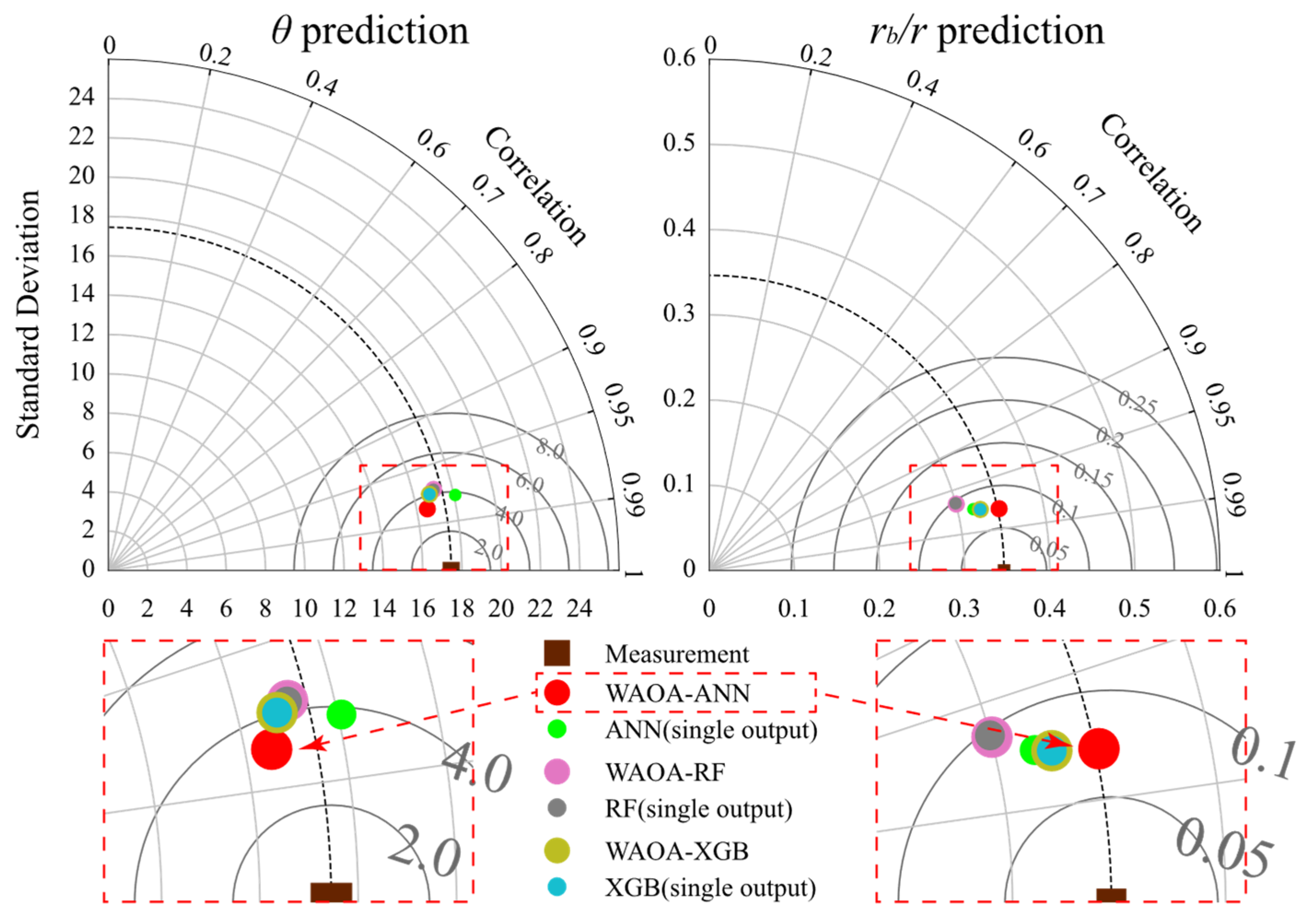
Given that the performance of the three hybrid multi-output models is relatively similar, the comparison of their distributions based on the scatterplot may not distinctly distinguish between the model performances. To provide a clearer assessment, the model performance is further illustrated using a Taylor diagram. This diagram facilitates a visual comparison of the three evaluation metrics (R², RMSE, and standard deviation) of the models in a single image.

In a Taylor diagram, the closer the data points are to the measurement point, the better the performance of the model they represent. Meanwhile, to evaluate the model’s capacity to leverage potential relationships between outputs, single-output ANN, RF, and XGBoost models were constructed with identical hyperparameter settings for comparative analysis. Figure 11 presents the Taylor diagram of the prediction performance of different models on the test set. As can be seen from the figure, the WAOA-ANN model is closest to the measure point in both $\theta$ and $r_b/r$ prediction. Additionally, there is a notable enhancement in the prediction performance compared to the single-output ANN model. For the WAOA-RF and WAOA-XGBoost model, on the one hand the predictive performance of the model on the test set is weaker than the WAOA-ANN model. On the other hand, the predictive performance of the multi-output RF and XGBoost models is in close agreement with that of the single-output models.

This demonstrates the strong generalization performance of the WAOA-ANN model, as well as its effective utilization of the potential connection between borehole breakout angle and depth. In comparison to the single-output ANN model, the WAOA-ANN model demonstrates superior prediction performance and requires fewer training resources for predicting the angle and depth of borehole breakout. For the WAOA-RF and WAOA-XGBoost models, there is no significant improvement compared to the single-output RF and XGBoost models. Additionally, their hyperparameters result in large model sizes, making the training process time-consuming and memory intensive, offering no practical advantage over the single-output RF and XGBoost models. Based on the comparative analyses of the models, the WAOA-ANN model is recommended for predicting borehole breakout size. Furthermore, the WAOA-ANN model undergoes further sensitivity analyses to explore the impacts of various input features on borehole breakout size.

4.3. Sensitivity Analysis

SHAP (SHapley Additive exPlanations) is a commonly employed model interpretation technique rooted in the concept of Shapley values from game theory [61,62,63,64]. It quantifies the contribution of input features to the model output through SHAP values. Analysis conducted with SHAP allows for the assessment of feature influence from both global and local perspectives, offering a more intuitive interpretation of model prediction outcomes. Furthermore, based on SHAP analysis results, adjustments to feature sizes can be made more scientifically and effectively to achieve target output values, serving as a crucial reference for design purposes.

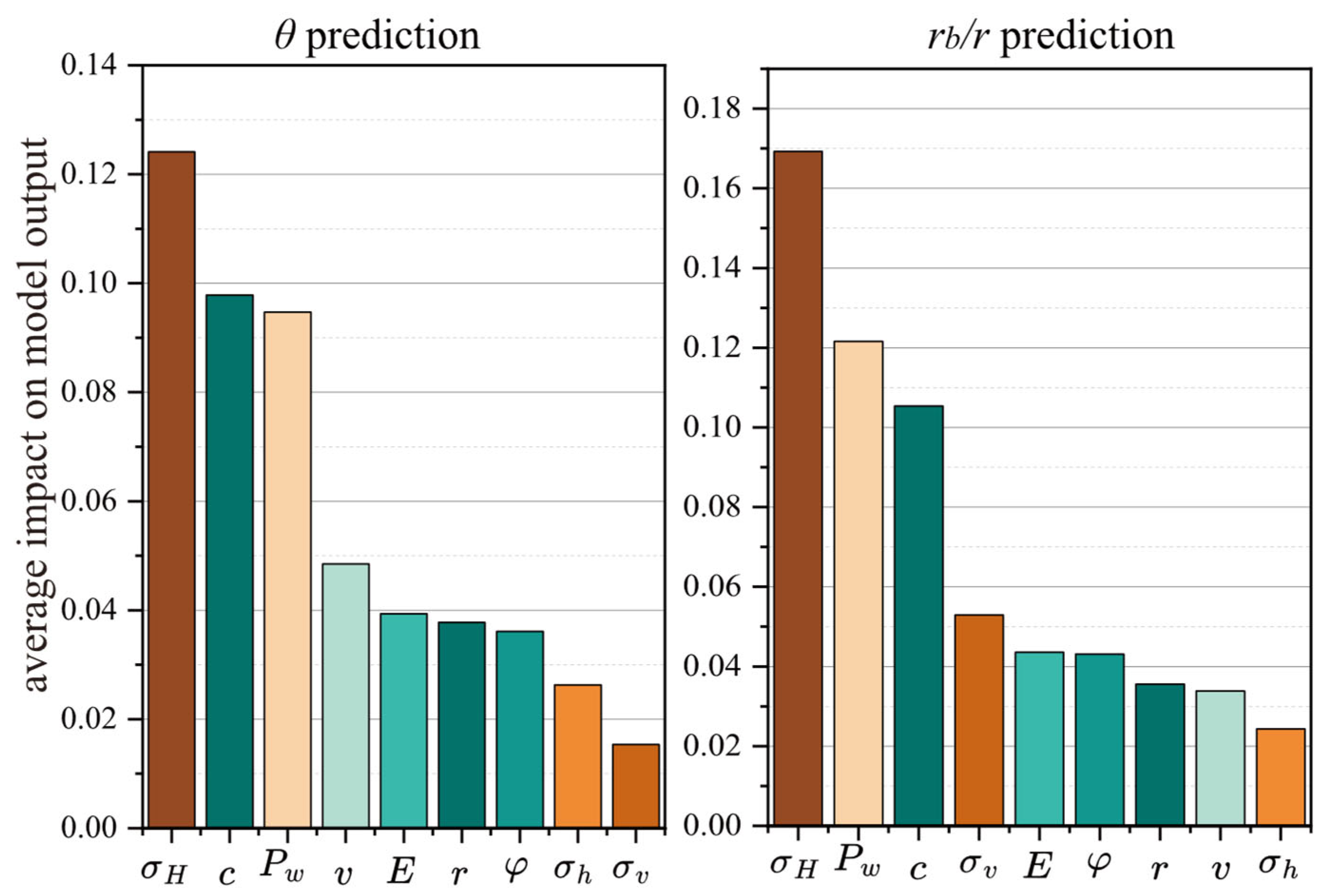
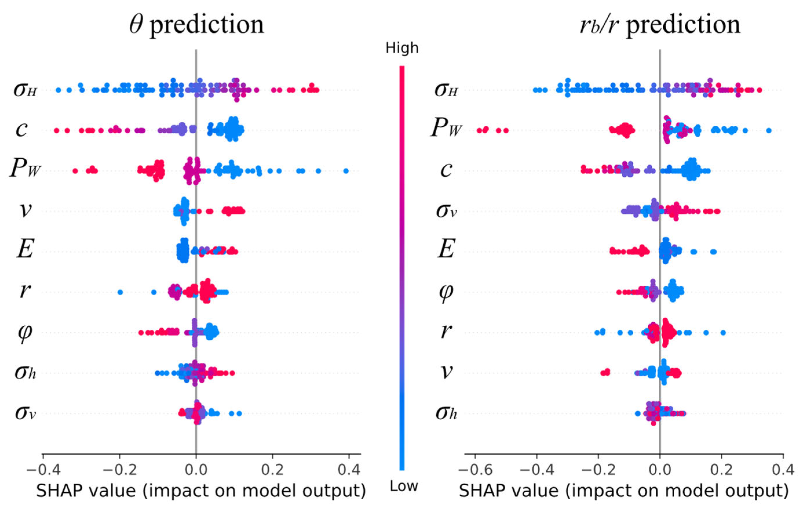
The WAOA-ANN model input feature impact rankings obtained based on SHAP analysis are shown in Figure 12. For the prediction of $\theta$, the ranking of the input feature’s impact on the output is ${\sigma }_H>c>P_w>\nu >E>r>\phi >{\sigma }_h>{\sigma }_v$ and for the prediction of $r_b/r$, the ranking is ${\sigma }_H>P_w>c>{\sigma }_v>E>\phi >r>\nu >{\sigma }_h$. The impact of input features on the output (promoting or reducing) changes with the value of the feature, and Figure 13 demonstrates the impact of different features on the WAOA-ANN output. From the figure, it can be seen that $\theta$ is positively correlated with ${\sigma }_H,\nu ,E,{\sigma }_h$, negatively correlated with $c,P_w,\phi ,{\sigma }_v$, and has a complex relationship with the $r$. $r_b/r$ is positively correlated with ${\sigma }_H,{\sigma }_v$, negatively correlated with $P_w,c,E,\phi$, and has a complex relationship with the $r,\nu ,{\sigma }_h$.

5. Conclusions

Borehole breakout, as a critical factor influencing borehole quality, has consistently attracted significant attention from researchers. This study collected a total of 501 datasets from numerical simulations and physical experiments, encompassing in situ stress, borehole dimensions, rock properties of the borehole wall, and mud pressure in the borehole as input features, with borehole breakout size as the output data. Three hybrid multi-output models (WAOA-ANN, WAOA-RF, WAOA-XGBoost) were developed using ANN, RF, and XGBoost as base algorithms, augmented by the WAOA optimization technique. The predictive performance of these models was compared and analyzed, while a single-output model was constructed to further assess the efficacy of the multi-output framework. The principal findings of this investigation are delineated below:

(1) All three hybrid multi-output models exhibit excellent prediction performance for borehole breakout size. Particularly, the WAOA-ANN model demonstrates consistent performance across both the training and test sets, surpassing WAOA-RF and WAOA-XGBoost on the test set (for $\theta$ training (test): R² = 0.9906 (0.9819), MAE = 0.0095 (0.0142), VAF = 0.9803 (0.9629), RMSE = 0.018 (0.0244); for $r_b/r$ training (test): R² = 0.9839 (0.978), MAE = 0.0167 (0.0208), VAF = 0.9679 (0.9556), RMSE = 0.0284 (0.0334)). Consequently, the WAOA-ANN model is deemed to possess superior prediction capabilities and stronger generalization ability.

(2) The WAOA-ANN model effectively leverages the potential correlation between borehole breakout sizes, resulting in a substantial enhancement in prediction performance compared to the single-output model. Conversely, WAOA-RF and WAOA-XGBoost exhibited no improvement in performance relative to the single-output model with identical hyperparameter settings, while also increasing the computational resource requirements of the model.

(3) The sensitivity analyses conducted on WAOA-ANN indicate that for both $\theta$ and $r_b/r$, ${\sigma }_H$ exhibits the highest sensitivity. However, there exists a considerable disparity in the rankings of input features concerning the impact on $\theta$ and $r_b/r$ ($\theta$: ${\sigma }_H>c>P_w>\nu >E>r>\phi >{\sigma }_h>{\sigma }_v$, $r_b/r$: ${\sigma }_H>P_w>c>{\sigma }_v>E>\phi >r>\nu >{\sigma }_h$). Additionally, variations are observed in the correlation of the same feature with $\theta$ and $r_b/r$. For instance, ${\sigma }_v$ displays a positive correlation with $\theta$ but a negative correlation with $r_b/r$. Similarly, $\nu$ and ${\sigma }_h$ exhibit a positive correlation with $\theta$ but a nonmonotonically correlation with $r_b/r$.

In conclusion, all three hybrid multi-output models developed achieved effective prediction of borehole breakout size, but only the WAOA-ANN model successfully demonstrated the advantages of the multi-output structure and performed better in terms of overall prediction performance. Therefore, the obtained WAOA-ANN is considered to be an effective hybrid multi-output model for borehole breakout size prediction. It is important to note that prediction results may be biased if the input feature values used exceed the range of the dataset in this paper. Hence, subsequent studies may consider covering a more comprehensive range of eigenvalues to enhance the robustness of the predictions.