Layer Contour Geometric Characterization in MEX/P through CIS-Based Adaptive Edge Detection

Abstract

The industrial adoption of material extrusion of polymers (MEX/P) is hindered by the geometric quality of manufactured parts. Contact image sensors (CISs), commonly used in flatbed scanners, have been proposed as a suitable technology for layer-wise characterization of contour deviations, paving the way for the application of corrective measures. Nevertheless, despite the high resolution of CIS digital images, the accurate characterization of layer contours in MEX/P is affected by contrast patterns between the layer and the background. Conventional edge-recognition algorithms struggle to comprehensively characterize layer contours, thereby diminishing the reliability of deviation measurements. In this work, we introduce a novel approach to precisely locate contour points in the context of MEX/P based on evaluating the similarity between the grayscale pattern near a particular tentative contour point and a previously defined gradient reference pattern. Initially, contrast patterns corresponding to various contour orientations and layer-to-background distances are captured. Subsequently, contour points are identified and located in the images, with coordinate measuring machine (CMM) verification serving as a ground truth. This information is then utilized by an adaptive edge-detection algorithm (AEDA) designed to identify boundaries in manufactured layers. The proposed method has been evaluated on test targets produced through MEX/P. The results indicate that the average deviation of point position compared to that achievable with a CMM in a metrology laboratory ranges from 8.02 µm to 13.11 µm within the experimental limits. This is a substantial improvement in the reliability of contour reconstruction when compared to previous research, and it could be crucial for implementing routines for the automated detection and correction of geometric deviations in AM parts.

1. Introduction

Additive manufacturing (AM) allows for the creation of objects by building them layer by layer. This original approach has generated an entirely new category of manufacturing processes distinct from traditional methods based on material solidification (such as metal casting or plastic injection molding), metal forming (such as rolling or sheet metal bending), or material removal (such as turning or electrical discharge machining) [1,2,3]. The fundamental aspects of AM processes are currently being standardized by the ASTM International and the International Organization for Standardization (ISO) [4]. Material extrusion of polymers (MEX/P) stands as one of the most widely utilized AM processes, mainly because of its user-friendly nature and the economical feedstock costs [5]. Nevertheless, the quality of MEX/P parts still fall short when compared to other conventional alternative processes, especially when it comes to serial manufacturing [6]. Particularly, issues regarding the dimensional and geometric quality of parts hamper the widespread industrial adoption of MEX/P [5,6,7]. The dimensional quality of MEX/P parts has been extensively studied [8,9,10,11,12,13]. Efforts to enhance the quality of manufactured parts have been focused on two fronts: adjusting process parameters [8,9,10] and refining the input geometry [11,12,13]. In both cases, retrieving accurate and dependable information regarding the actual geometries of manufactured parts is imperative. Moreover, checking the effectiveness of corrective measures also demands the capability of quantifying the deviations between actual (manufactured) geometries and the theoretical expectations.

In MEX/P, dimensional and geometric verification is typically conducted similarly to conventional manufacturing processes. This involves using measurement and scanning methods, either contact or non-contact, after a part has been manufactured [14,15,16]. However, the layer-by-layer nature of AM manufacturing opens the possibility of verifying the deposited geometry shortly after each layer has been fabricated without having to wait for the part to be completely manufactured [17]. This capability, which relies on the integration of in-machine geometry characterization systems, allows for the acquisition of layer-wise information, enabling the early adjustment of process parameters or even the application of geometry compensation strategies [18].

Layer-wise monitoring has been applied in MEX/P by means of three main sensing technologies: thermal sensing [19], 2D vision [20], and 3D vision [21]. Each technology has its own advantages and disadvantages. For instance, temperature-field sensors lack sufficient spatial resolution to be used in dimensional or geometric verification of a part, while integrating sensors for 3D scanning can be a complex task due to their size and weight. On the other hand, 2D vision systems tend to be more compact and lighter, making their integration into commercial MEX/P machines relatively simpler [20,22]. However, the distortion introduced by the optics, along with insufficient spatial resolution, makes these methods more commonly used for defect localization and characterization [22] rather than for the precise measurement of dimensional or geometric deviations.

Flatbed scanners based on contact image sensors (CISs) have certain characteristics that make them a viable option for integrating 2D vision systems for layer-wise inspection tasks in MEX/P machines. Although these types of devices are commonly used for scanning documents and photographs, they have also been employed for contour detection in nearly flat [23] and three-dimensional objects [24]. Flatbed scanners have been used in AM to characterize irregularities in the deposition of metal powders in PBF/M [25], to characterize distortion of parts in MEX/P [26], and even to compensate for machine errors [27].

Our team has worked on two crucial aspects of the use of CISs in MEX/P applications. The first aspect deals with the accuracy of layer contour detection for the geometric characterization of manufactured objects [28,29,30]. The second aspect focuses on the integration of sensors into MEX/P equipment for process monitoring [30,31,32]. Accurately identifying contour points in digitized images is essential for verifying the dimensional and geometric parameters of the fabricated layer. Initial efforts focused on compensating for image distortion [28]. It was found that such distortion exhibits differential characteristics between the scanning direction ($\overrightarrow{v}$) and the direction of the photodetector array ($\overrightarrow{a}$). Beyond this circumstance, it was also found that global compensation techniques [26] are insufficient to achieve precision levels in point localization comparable to those attainable in coordinate-based metrology. Consequently, a local distortion adjustment (LDA) algorithm was developed. Enhancing the results of global techniques, the LDA allowed for very precise contour reconstruction under high target-to-background contrast scenarios.

Focusing on contour identification in images, this complex task has been addressed through various edge-detection algorithms, such as those proposed by Roberts [33], Sobel [34], and Prewitt [35]. However, the Canny algorithm [36] stands out as the most-employed algorithm [37]. Nevertheless, these algorithms and those based on second derivatives, like zero-crossing or the Laplacian of Gaussian, were not designed for the dimensionally precise and unambiguous contour detection required in industrial-level dimensional verification and quality control. Instead, they were developed for tasks such as feature extraction [38], image segmentation [39], object recognition [40], and image enhancement [41].

Contour characterization in AM using conventional algorithms has been previously addressed in several works [42,43,44,45,46]. Thus, Heinl et al. compared different algorithms (Sobel and Canny) based on qualitative impressions that evaluate the completeness of contour reconstruction in SLS-manufactured parts [42]. Özsoy et al. reported minimum average errors in the range of tenths of a millimeter when measuring layers with a CCD in powder bed fusion manufacturing [43]. Similar results were reported by Amindazeh and Kurfess, who noted a maximum point-to-point error of 0.480 mm [44]. Lerchen characterized the layer contour in PBF images where the layer-to-background contrast pattern appeared to be nearly uniform [45]. Nevertheless, quality characterization in AM through image analysis is mostly focused on the detection of coarse defects [46]. From the analysis of these works, it can be deduced that the contour characterization techniques currently applied in AM are focused on the detection of coarse deviations, mainly in the range of tenths of a millimeter. This level of resolution in error characterization is conditioned by the quality of the optical equipment used and the quality of the geometric reconstruction provided by conventional edge-detection algorithms.

One of the main problems when using conventional algorithms for tasks that require precise dimensional and geometric characterization of layer contours is their high sensitivity to non-uniformity in contrast patterns or variations in grayscale [42]. This issue has been addressed in two studies [29,30], which revealed that optimizing the parameters of conventional contour detection algorithms (such as Canny, Prewitt, Sobel, etc.) can enhance the results of contour point identification in terms of both coverage and precision. However, it was also observed that these algorithms can only provide accurate reconstructions of layer contours when the entire contour shows substantial and uniform contrast against the background. They struggle to offer a comprehensive and accurate reconstruction when contrast patterns exhibit significant asymmetries depending on the local orientation of the contour [29]. Essentially, a single processing configuration cannot simultaneously achieve satisfactory reconstruction in areas with heightened contrast and areas with poor contrast within the same image. As a result of these findings, two potential strategies were proposed: the formulation of an adaptive procedure for contour detection and the development of scanning devices with controlled directional illumination.

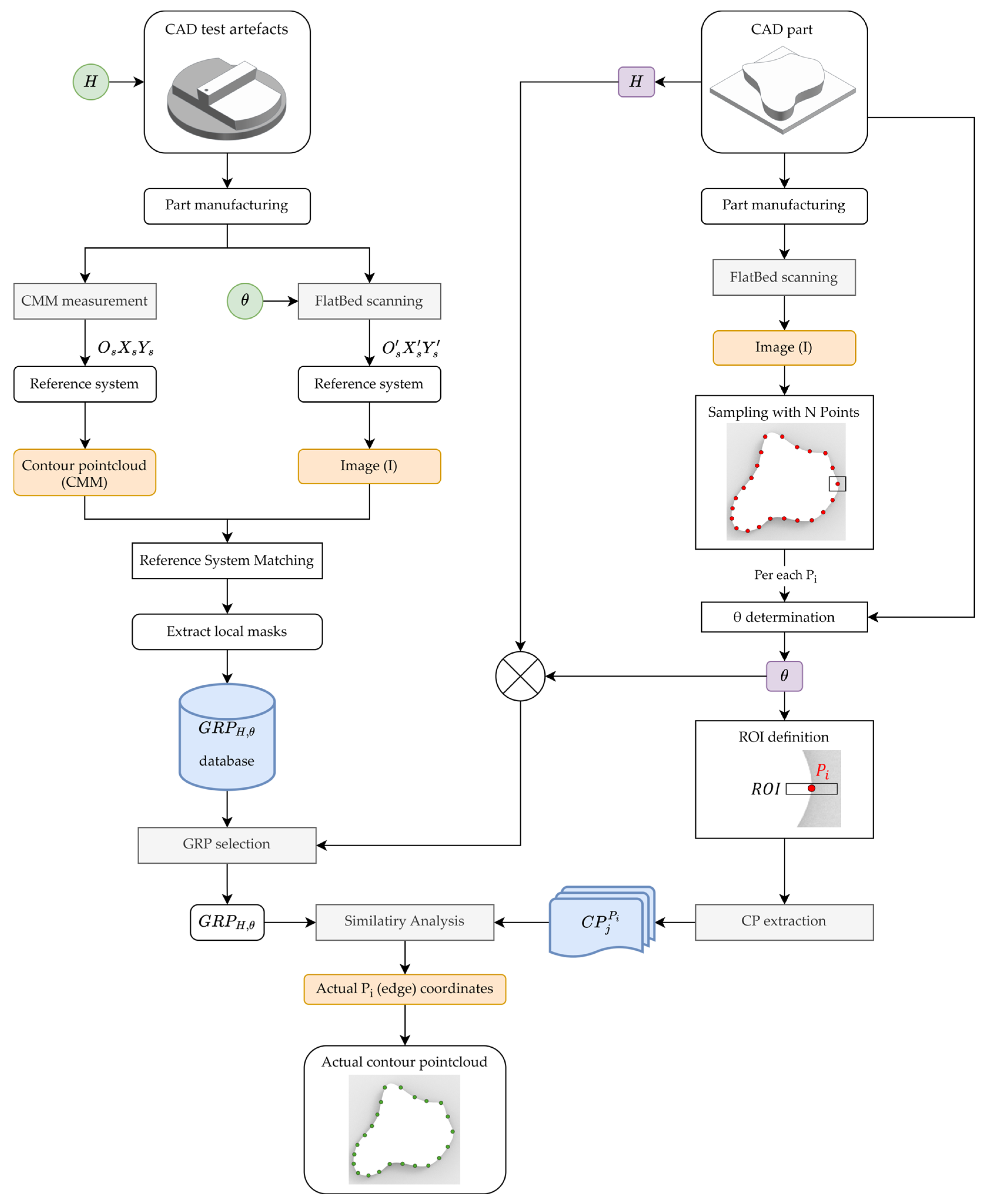
The present work focuses on implementing the first of the aforementioned strategies by devising a procedure for edge detection that is tailored for non-uniform contrast patterns. The premise is that the location of a layer contour point can be determined by comparing the local grayscale pattern surrounding its theoretical position with a pre-existing reference pattern. Accordingly, we utilized a series of orientable test artefacts with contours at various layer-to-background distances while also allowing for setting different contour-to-illumination orientation angles. The test artefacts are digitized using a coordinate measuring machine (CMM) to accurately determine the position of individual contour points. A digital image is captured using a CIS, enabling the calculation of contour point positions in pixel coordinates from the CMM data. Subsequently, local grayscale patterns corresponding to the location of each contour point are extracted and grouped in a gradient reference pattern (GRP) database. Then, when characterizing the contour of a manufactured part, its approximate location can be predicted from the CAD file. Accordingly, the approximate positions of individual tentative contour points can be established beforehand in the digital image captured with the CIS. A set of one-dimensional regions of interest (ROIs) can then be defined around those tentative contour points. Finally, a set of candidate patterns (CPs) are extracted from the ROIs, and their similarity to the correspondent GRP is subsequently evaluated. The most similar CP for a given tentative contour point will then be used to determine the exact location of the actual contour point. This procedure provides precise identification of contour point locations in the target layer and is less susceptible to being influenced by local characteristics of the contrast pattern.

The proposed method diverges from conventional approaches in three significant aspects:

• Contour point identification relies on data obtained from test artefacts measured with a CMM, whereas conventional approaches stand alone, and the dimensional accuracy of contour reconstruction is not even relevant.
• Edge detection is customized through adaptive processing that considers the local characteristics of the layer-to-background pattern. This approach differs from methods that process entire images with a single algorithm configuration.
• Each local search yields a single contour point, differing from the multiple candidates typically provided by most edge-detection algorithms.

In summary, the approach presented in this work has been tailored to overcome the limitations of conventional algorithms, such as Canny or Prewitt, in situations where the layer-to-background contrast is highly uneven. While reported errors in related works are in the range of tenths of a millimeter [43,44], our goal is to reduce these discrepancies for MEX/P parts through the optimization of conventional algorithms [29]. This means lowering quantification errors to below 50 µm in non-uniform contrast scenarios.

The subsequent sections of this paper are structured as follows: after the introduction in Section 1, Section 2 provides a general overview of the proposed adaptive edge-detection algorithm (AEDA); the method for constructing the reference database is outlined in Section 3; Section 4 elucidates how contour points are identified in a manufactured part; a practical example of the proposed procedure is presented in Section 5; the results are discussed in Section 6; and, finally, Section 7 summarizes the conclusions of this work.

2. Fundamentals of the AEDA

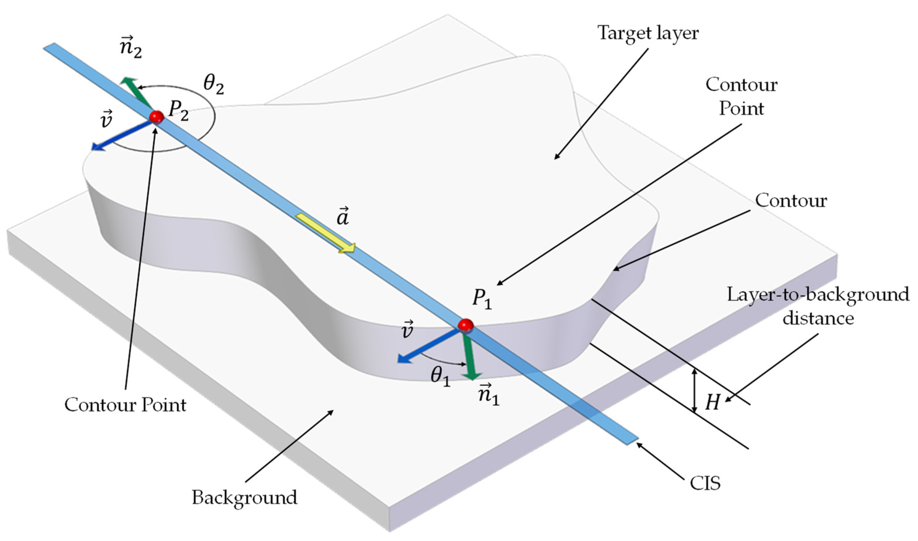
As outlined in the previous section, this work is based on the premise that the relative location of a layer contour point can be established by comparing the local grayscale pattern around the expected or theoretical position with a previously obtained reference pattern. Each local grayscale pattern along the layer contour is influenced by various factors, such as the optical characteristics of the deposited material, the vertical distance between the target layer and the surrounding background ($H$), or the relative orientation ($\theta$) of the normal to the contour at the theoretical point (${\overrightarrow{n}}_i$) and the scanning direction ($\overrightarrow{v}$) (Figure 1). Since the optical characteristics are unique for a given material, this factor should only be considered if different materials are to be used in the same part, which is not typically the case in MEX/P. Therefore, setting material considerations aside, the two primary factors influencing the characteristics of the grayscale pattern near a contour point ($P_i$) are $H$ and $\theta$. Notice that, due to its design, the CIS illuminates the scene with a series of LEDs preceding the array of photodiodes ($\overrightarrow{a}$), and, accordingly, the direction of the illumination opposes the scanning direction ($-\overrightarrow{v}$).

According to the detailed view depicted in Figure 2, the CIS, moving in the direction of vector $\overrightarrow{v}$, scans both the target layer and the background, capturing a digitized image of the part. At the position illustrated in the figure, the image ideally encompasses contour segments with two contour points ($P_1$ and $P_2$), delineating the precise boundary between the target layer and the surrounding background.

Figure 3 presents detailed views of actual contours obtained for different combinations of layer-to-background distances and contour orientations. At a given angle, increasing the layer-to-background distance enhances the contrast between the background itself and the target layer. This results in a less pronounced gradient at lower $H$ values, which would become more pronounced as $H$ increases. This issue arises from the diminishing light intensity over increasing distances due to spreading and attenuation phenomena. Consequently, the intensity of light reflected by the target layer becomes much higher than that reflected by the background. Similarly, variations in $\theta$ shall also affect the gradient. For instance, with a 0° orientation (where the scanning direction aligns with the normal to the contour at the point), the CIS illuminates the background first without any shadows cast by the material layers above. Conversely, a 180° orientation results in the uppermost layer casting a shadow on the background zone near the contour. Intermediate orientations between these extremes yield significant variability in the intensity gradient recorded by the CIS near the contour, as depicted in Figure 3.

Since the intensity gradient recorded in the image captured by the CIS varies depending on $H$ and $\theta$, the grayscale reference pattern can be anticipated for any given combination of both parameters ($GR{P}_{H,\theta }$).

Therefore, when analyzing a manufactured layer, an analysis of the distribution of the extracted CPs near each tentative contour point can be performed to determine which CP best matches the GRP corresponding to the specific combination of $H$ and $\theta$. In the context of this work, the grayscale patterns used are treated as n-dimensional row vectors, where each component has a grayscale intensity level on a scale from 0 to 255.

For a given tentative point upon a manufactured layer ($P_i$), each of the $j$ possible CPs extracted from the ROI will have an associated subset ($C{P}_j^{P_i}$). A similarity analysis between each $C{P}_j^{P_i}$ and the correspondent $GR{P}_{H,\theta }$ will provide the location of the actual contour point. Following this procedure for the whole set of tentative contour points, the edge will be finally characterized. Figure 4 provides a flowchart of the proposed AEDA.

3. Building a GRP Database

Every $GR{P}_{H,\theta }$ has an odd number of components, so that the central one corresponds to the theoretical transition between the target layer and the background. Each component in the $GR{P}_{H,\theta }$ contains an intensity value between 0 and 255 that corresponds to the grayscale value recorded for an individual pixel in the image digitized by the CIS (Figure 5). Accordingly, each row vector should describe the ideal distribution of grayscale levels along a linear segment centered on a contour point for a specific combination of $H$ and $\theta$.

The central component consistently marks the transition between the target layer and the surrounding background, ideally pinpointing the location of an individual contour point where the layer edge intersects a specified direction. Since the pixel arrangement in a digital image forms a rectangular matrix, inspection is considered only in two orthogonal directions: the scanning or vertical direction ($\overrightarrow{v}$) and the direction of the photodetector array or the horizontal direction ($\overrightarrow{a}$). Selection of the search direction will depend on the theoretical orientation of the contour at each contour point. Thus, vertical directions will be used for $135°\le \theta \le 225°$, $0°\le \theta \le 45°$, and $315°\le \theta \le 360°$. Similarly, horizontal directions will be used for $45°<\theta <135°$ and $225°<\theta <315°$. Building the GRP database requires accurately identifying which pixel corresponds to the exact location of the contour point. Accordingly, a set of test artefacts embodying different combinations of contrast conditions are required.

3.1. Test Artefacts

The design of test artefacts should be tailored to offer contours at various layer-to-background distances and different orientations. The experimental range established for the present work comprises variation in $H$ between 8 mm and 2 mm and a complete 360 range for $\theta$. Since it is impossible to materialize all possible combinations of $H$ and $\theta$, a reduced range was defined, including four possible levels for $H$ (2 mm, 4 mm, 6 mm, and 8 mm) and twenty-four levels for $\theta$ (0°, 15°, 30°, …, 345°). Intermediate combinations will require interpolation between GRPs. 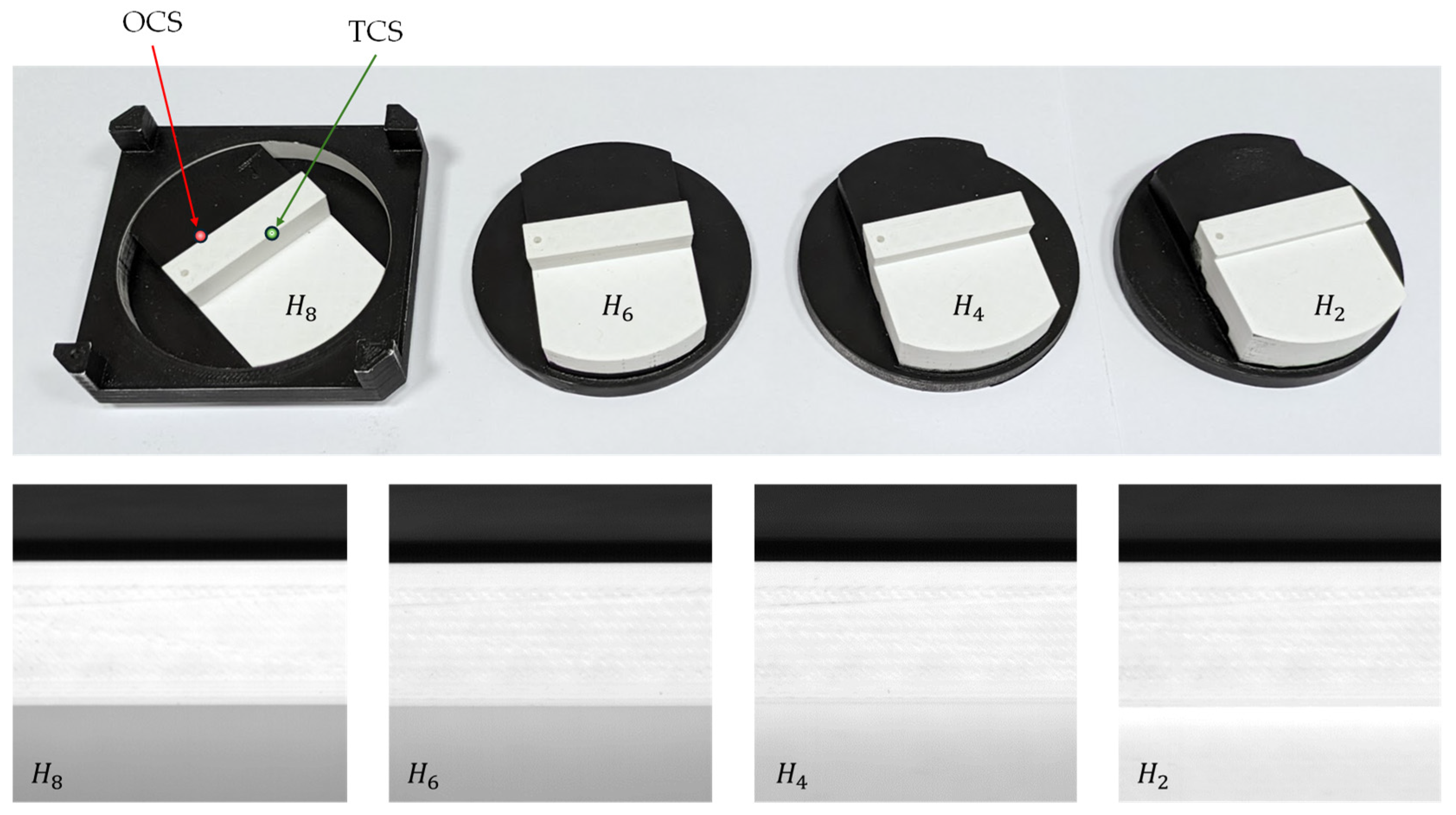However, despite the reduction in test levels, the possible combinations of the parameters $H$ and $\theta$ would yield a minimum of 96 test artefacts. To reduce the number of parts to be manufactured, a design based on two parts was chosen. The assembly consists of a rectangular base with reference elements like those used in [26], which can be easily positioned in the CIS’s work field, and a central rotating element, which embodies a specific value of $H$ (Figure 6).

The rotative central element presents a rectangular flat surface resembling an ideal target layer with the standard optical characteristics of the feedstock. One of the longest sides (the test-contrast side or TCS) of this surface materializes a specific value of $H$. On the other hand, the opposite side of this rectangular flat surface materializes an ideal optimal contrast situation (the optimal-contrast side or OCS), where the contrast achieved through an extensive gap between the target layer and the background was reinforced by painting the background black. By rotating the central element for each specimen in the CIS, images can be obtained for each of the 96 possible experimental combinations.

3.2. Manufacturing of Test Artefacts

Test artefacts were designed and manufactured in white BCN3D^® PLA in a Sigma MEX/P machine (BCN3D Technologies Inc., Barcelona, Spain). The standard manufacturing profile for a 0.1 mm layer resolution, given by the product’s supplier, was used (

Table 1. Configuration parameters used for manufacturing test artefacts.

Parameter	Value
Material	White BCN3D® PLA
Extruder temperature	200 °C
Layer height	0.1 mm
Flow rate	100%
Filament diameter	2.85 mm
Top/bottom pattern	Lines
Wall ordering	Outside—inwards

).

Once manufactured, the OCS background was painted black to minimize contrast-dependent issues. Figure 6 also provides individual images of the specimens as registered with the CIS for a $0°$ orientation, where differences between TCS backgrounds can be observed: the higher the $H$, the higher the contrast achieved.

3.3. CMM Digitization of Test Artefacts

The test artefacts were measured using a coordinate measuring machine (CMM), the DEA Global Image 09-15-08 (Hexagon AB, Stockholm, Sweden), with a contact touch-trigger probe. This machine was calibrated according to [47] with the maximum permissible error in length measurement, as in Equation (1):

$$MP{E}_E=2.2+3·L/1000 \left(\mathrm{\mu }\mathrm{m}\right) \left(L in \mathrm{mm}\right)$$

(1)

and the maximum permissible error in probing repeatability, as in Equation (2):

$$MP{E}_P=2.2 \left(\mathrm{\mu }\mathrm{m}\right)$$

(2)

Metrological operations regarding CMM digitization were performed using PC-DMIS^® (Hexagon AB, Stockholm, Sweden). Since the geometry of the target layer remains invariant regardless of the orientation, CMM digitization of points along the TCS and OCS was performed only once per test artefact. The initial step was to determine the Z axis, then the Y axis ($Y_s$), and finally the origin ($O_s$). After defining the local origin, two sets of ten individual contour points were measured for each test artefact. The first set consisted of ten contour points equally spaced along the TCS ($P_{i_{TCS}}$), while the second set comprised ten points equally spaced along the OCS ($P_{i_{OCS}}$). Once measured, each point was characterized by its $x$ and $y$ coordinates relative to the origin ($O_s$). Figure 7 illustrates the distribution of points digitized with the CMM.

3.4. Identification of Contour Points in the Digitized Images

Digital images of the test artefacts were acquired using a Perfection V39 EPSON flatbed scanner (Seiko Epson Corporation, Nagano, Japan), which integrates a CIS. Each test specimen was placed upside down on the scanner, with the target layer directly on the glass. Scanning was conducted at a resolution of 2400 dpi along both the scanning direction ($\overrightarrow{v}$) and the direction of the photodetector array ($\overrightarrow{a}$). As a result, grayscale images were obtained for each test combination, totalling 96 images.

Before the calculation of the GRPs, it was necessary to identify the reference system of the target layer in the digitized images. To this end, a small reference hole was included at the bottom of the target layer to address the problem of axis orientation associated with the symmetry of its rectangular geometry. The procedure (as depicted in Figure 8) is as follows: (a) detect the circle corresponding to the reference hole; (b) binarize the image using the Otsu algorithm with a threshold of 125 and identify the OCS (long side) and the orthogonal short side of the rectangular target; (c) define two search regions approximately located along the mentioned sides. Once these search regions are defined, the identification of individual contour points on both sides can be performed using the optimal parameters calculated in [29] for a high-contrast scenario: a Canny filter with a noise filter size ($S_f$) of 19 and a threshold ($T$) of 110. After these points are calculated, they are used to define both the $X_s$ and $Y_s$ axes following the same procedure as would be used in a CMM. This reference system (d) will correspond to the one calculated with the CMM.

Once the local reference system of the target layer has been positioned in the image, the points digitized with the CMM can be translated from the coordinate system of the measuring machine (in mm) to the system of the digitized image (in pixels). However, since an image captured by an optical digital system like a CIS is a distorted representation of reality, it is essential to apply a transformation that accounts for this distortion when adjusting the coordinates of contour points. As explained in [28], global transformations do not fully address the distortion issue, making a local compensation approach a more viable option. In this work, the LDA method described in [28] was employed to address image deformations.

Utilizing LDA enables the placement of the calculated coordinates for each point ($P_{i_{TCS}}$) in the image, thereby facilitating the identification of the grayscale pattern in the local vicinity of the contour point (Figure 9).

3.5. Calculation of GRPs

Once this process is completed, a representative $GR{P}_{H,\theta }$ can be finally calculated considering 10 individual local masks: one for each CMM-digitized TCS contour point. The orientation of these masks is consistent with the criterion for angular ranges established at the beginning of this section. Accordingly, the intensity value ($I$) of each pixel ($j$) in $GR{P}_{H,\theta }$ ($I_{H,\theta }^j$) will be calculated as the average of the intensity values ($I_{H,\theta ,i}^j$) collected for the corresponding $j$-th pixel in the $i$-th individual masks (Figure 10), following Equation (3).

$$I_{H,\theta }^j=\frac{1}{n}·{\displaystyle \sum }_{i=1}^n{I}_{H,\theta ,i}^j$$

(3)

Following this procedure, a GRP database was constructed. The size of $GR{P}_{H,\theta }$ ($n$) was set at 51 pixels, which for a 2400 dpi resolution is equivalent to a length of 539.75 µm. The angular resolution of the database was set to 15°. Accordingly, the database used in this work consists of 96 GRPs (24 GRPs for each layer-to-background distance). Figure 11 provides four independent representations of the $GR{P}_{H,\theta }$, arranged along their respective angular orientations.

4. Identification of Contour Points in a Manufactured Part

The process of identifying contour points on a manufactured component begins with digitizing the layer to be inspected using the CIS. The captured image undergoes processing with LDA to compensate for distortions, enabling the conversion of pixel coordinates to component coordinates. To achieve this, it is crucial to establish a reference system for the component, or, more precisely, for the target layer.

Determining the reference system from the image involves a procedure like the one used for locating the target-layer origin in reference patterns, as described in the preceding section. However, this determination depends on the geometric attributes of each layer. Consequently, after applying LDA, translating the theoretical positions (obtained from the CAD file) of the contour points in the image becomes straightforward, yielding a set of tentative points close to where the actual contour points should lie (see Figure 12).

This procedure yields a collection of tentative points ($P_i$), for which their position in the image in pixel coordinates, the theoretical contour orientation ($\theta$), and the distance between the target layer and the local background ($H$) at each point are already known. Thus, adhering to the same criterion for the vertical/horizontal orientation of GCPs described in the preceding section, it becomes feasible to define the $RO{I}_{P_i}$ (Figure 12).

Each $RO{I}_{P_i}$ will have a size ($m$) significantly larger than the size ($n$) of the reference vector $GR{P}_{H,\theta }$, allowing for the extraction of every possible CP and its corresponding $C{P}_j^{P_i}$ vector, also $n$-sized. As a rule, $m$ should be large enough to ensure that the position of the tentative point does not differ significantly from the position of the actual contour point to the extent that the latter falls outside the $RO{I}_{P_i}$, thereby impeding its accurate identification. Given the typical dimensional errors documented in studies such as those published by Minetola [14], a region of interest greater than 0.5 mm should be sufficient in most cases, although larger lengths would also be adequate.

The degree of similarity between each $C{P}_j^{P_i}$ and the corresponding $GR{P}_{H,\theta }$ is evaluated by means of the Euclidean distance ($d$), following Equation (4).

$$d\left(C{P}_j^{P_i},GR{P}_{H,\theta }\right)=\Vert C{P}_j^{P_i}-GR{P}_{H,\theta }\Vert$$

(4)

The closer the value of $d$ is to 0, the more similar both vectors are. By evaluating the value of $d$ across the $RO{I}_{P_i}$, the algorithm searches for the vector that yields the minimum value, thereby assigning the location of the actual contour point.

In the example provided in Figure 13, an $RO{I}_{P_i}$ consisting of 51 pixels is analyzed using a window size of seven pixels. With this length, the first assessable position is centered on pixel 4 ($C{P}_4^{P_i}$), which retrieves a $d$ value of 1.459. Then, the procedure moves to the next position (pixel 5) to extract $C{P}_5^{P_i}$ and calculate its $d$ value, and it will continue up to pixel 48, since this is the last assessable position given this window size. In this example, the candidate pattern centered in the 25th pixel yields the minimum value for the Euclidean distance (0), and, consequently, the contour point location will be assigned to that position. This procedure should be repeated for all the previously defined tentative points along the theoretical layer contour, retrieving a collection of contour points. The final step of the algorithm involves applying an outlier filter to remove false positives related to phenomena such as ghostly features, small disturbances, and hindrances.

5. Case Study

In this section, we present a case study to evaluate the degree of improvement over generic edge-detection algorithms based on testing samples like those used in [29].

5.1. Manufacture and Digitization of the Test Specimens

Following [29], the test targets are circular contours corresponding to the top layer of inverted conical frustums. Four test specimens were manufactured resembling the layer-to-background distances previously tested: $H_8,H_6,H_4, \mathrm{and} H_2$ (Figure 14).

Once manufactured, all four specimens were digitized using the scanner mentioned in Section 3.4, with a resolution of 2400 dpi. Additionally, they were also measured with the CMM mentioned in Section 3.3. Figure 15 shows the digital images obtained for each target. Due to the scanning direction and the geometric arrangement of illumination in the CIS, the top layer casts shadows in the upper region, resulting in a darker background compared to other orientations. Conversely, the lower region of the background receives unobstructed light, resulting in a brighter appearance. This effect is also influenced by the layer-to-background distance. Specifically, the background of the $H_2$ specimen is brighter in the lower region than in the adjacent area of the target layer.

5.2. Contour Reconstruction of Test Targets

According to the proposed procedure, it is necessary to position the $P_i$ tentative points in the image to identify the $RO{I}_{P_i}$. This positioning requires locating an identifiable part origin in the digital image. In this work, test targets were provided with a reference hole at the center of the target layer. This hole is identified in the digital image using the Hough algorithm [48], obtaining the pixel coordinates of its center, which serves as a valid coordinate origin for the tentative points. The theoretical coordinates of the $N$ tentative points are then transformed into pixel coordinates through the application of LDA, aligning them with the image of the manufactured part.

In this work, a total of 720 tentative points were used. Given that the selected test geometry was a circumference, the angular resolution for the dimensional and geometric characterization of the contour was 0.5°. Since the reference database was constructed with a 15° resolution, an interpolation procedure was applied. Accordingly, each pixel ($n$) of the $GR{P}_{H,\theta }$ corresponding to angle $\theta$ was calculated from the $n-th$ element of the adjacent $GR{P}_{H,\theta }$ vectors defined for the preceding and subsequent angles. Figure 16 shows an example of the interpolation between $GR{P}_{H_2,150}$ and $GR{P}_{H_2,165}$ to construct an interpolated $GR{P}_{H_2,160}$.

For each $P_i$, an $RO{I}_{P_i}$ is defined according to the orientation rules outlined in Section 3. In this work, the length of the ROIs ($m$) was calculated using Equation (5).

$$m=2·\Vert GR{P}_{H,\theta }\Vert -1=2·n-1=101$$

(5)

Consequently, each ROI was 1.069 mm long. The procedure then extracted all the n-sized $C{P}_j^{P_i}\mathrm{s}$, and Equation (4) was applied to determine each candidate’s similarity to the $GR{P}_{H,\theta }$. By repeating this process for all tentative points, a cloud of contour points was obtained, providing a discrete representation of the target layer’s contour.

5.3. Results

Figure 17 shows the radial deviations $(R_d\mathrm{s})$ between the actual positions of the contour points and the theoretical ones. These deviations are illustrated for both verifications performed with the CMM (orange line) and those obtained with the described procedure (blue line).

As shown, the identification of contour points using the proposed method covers the entire target layer, and the radial deviations are closely aligned with those obtained using the CMM.

To quantify how comparable the obtained results are to a trusted reference, the same quality indicators defined in [29] were used. The coverage factor ($C_f$) represents the completeness of test-target reconstruction. The circular contour is divided into angular sectors, and $C_f$ is defined as the percentage ratio of the number of sectors containing at least one valid contour point ($n_{S_v}$) to the total number of sectors considered ($n_{S_T}$) (360 for this research), as shown in Equation (6). The average of radial deviations ($\overline{D}$) is calculated as the mean absolute value of the deviations between the contour points obtained through image processing and those measured with the CMM, previously grouped into those 360 sectors, following Equation (7). Finally, the standard deviation of radial deviations (${\sigma }_D$) represents the variability of the radial deviations along the contour, calculated as in Equation (8).

$$C_f=\frac{n_{S_v}}{n_{S_T}}·100=\frac{n_{S_v}}{360}·100$$

(6)

$$\overline{D}=\frac{1}{n}·{\displaystyle \sum }_{i=1}^n\left(R_{d_i}\right)$$

(7)

$${\sigma }_D=\sqrt{\frac{1}{n-1}·{\displaystyle \sum }_{i=1}^n{\left|R_{d_i}-\overline{D}\right|}^2}$$

(8)

According to

Table 2. Quality indicators for each test artefact.

	${\mathit{H}}_8$	${\mathit{H}}_6$	${\mathit{H}}_4$	${\mathit{H}}_2$
$C_f \left[\%\right]$	100	100	100	100
$\overline{D} \left[\mathrm{\mu }\mathrm{m}\right]$	11.01	8.02	11.27	13.11
${\sigma }_D \left[\mathrm{\mu }\mathrm{m}\right]$	8.35	8.60	12.21	13.35

, the proposed method allows nearly full coverage, even for low-contrast specimens. Moreover, the average of the radial deviations is lower than 14 µm for each artefact, with a maximum standard deviation of 13.35 µm for the worst-case scenario ($H_2$).

6. Discussion

The use of CIS systems could enable the thorough digitization of individual layers in MEX/P components. Although an accurate characterization of layer contours from digital images is hindered by several factors, issues such as image distortion can be mitigated through global or local compensation methods. However, challenges persist with factors like the contrast pattern structure between the layer contour and its background, affecting the performance of popular detection algorithms such as Canny and Sobel. This problem is particularly pronounced when the proximity between the layer and the background leads to noticeable asymmetries in those contrast patterns. The proposed AEDA leverages the peculiarities of contour characterization in MEX/P by minimizing errors in the precise identification and localization of layer contour points within images captured by a CIS. The AEDA operates on the principle that similar contrast scenarios will produce consistent grayscale patterns between the target layer’s contour and the surrounding background.

The results presented in Section 5 indicate that the average deviation of point position was comparable to that achievable with a CMM in a metrology laboratory, ranging from 8.02 µm to 13.11 µm within the experimental limits. These results are sufficiently precise for quality characterization and for implementing compensation strategies, considering that typical dimensional errors in MEX/P are measured in tenths of millimeters for parts similar in size to the test targets used in this study [14]. Furthermore, the proposed AEDA outperforms the results obtained for the worst-case-scenario parts discussed in [29]. Specifically, in that work, the average of radial deviations ($\overline{D}$) was 54.9 µm for an $H_2$ specimen (using Canny processing with $T=10$ and $S_f=1$) and 55.97 µm for an $H_4$ specimen (using Roberts processing with $T=5$ and $S_f=1$). This demonstrates that the AEDA significantly surpasses the best results achieved with conventional edge-detection algorithms [40,41], even when the optimal combination parameters $T$ and $S_f$ were used [29].

One particularly beneficial characteristic of this implementation is that an approximate expected location of actual layer contours can be established beforehand, given that typical positional errors of individual geometric features in MEX/P are on the order of tenths of a millimeter. Consequently, the expected position of contours within the digitized image is accurate enough to identify a set of tentative points, ensuring that the actual contour points will be situated nearby. This advantageous feature of layer-wise CIS scanning contrasts with typical applications of conventional edge-detection algorithms, where the approximate location of edge contours is unknown beforehand and the algorithms must process the image as a whole. The results demonstrate a consistent improvement in the quality of the reconstruction, achieving two objectives. Firstly, it eliminates the necessity to choose an optimal combination of edge-detection method and processing configuration. The proposed method is, in this regard, more robust. It also reduces the uncertainty of contour point identification, as the algorithm yields only one valid (optimal) contour point location for each local search area. In contrast, conventional edge-detection algorithms often produce multiple-point detections due to the complexity of contrast patterns.

As a downside, the proposed procedure entails the execution of a preliminary phase of experiments for the characterization of the reference masks. This characterization may become time-consuming when additional factors, such as the type of material or the potential interference in the shadow pattern caused by complex contours, are introduced. Similarly, an increase in the discretization of the number of test levels will demand a greater experimental effort. Additionally, the challenges associated with the integration of CIS sensors into the machinery should not be underestimated, nor should the impact of external light sources on the quality of the results. Moreover, this study has certain limitations related to the manufacturing equipment, feedstock, test-target geometry, and the FBS model. None of these inconveniences are, according to the research team’s judgment, insuperable, but they should not be ignored or downplayed. Since the procedure includes the creation of a GRP database, variations in the manufacturing machine or the feedstock will require the manufacture and digitization of specific test artifacts, and these limitations should not pose a problem. Similarly, FBS particularities will be taken into account during the generation of the LDA parameters. However, the evaluation of non-circular geometries will require adapting the procedure and selecting alternative quality indicators that do not rely on radial differences. The development of a robust layer digitization system in MEX/P still requires CIS manufacturers to actively engage in integrating these sensors into production equipment. This integration could encompass an improved control of lighting during scanning, even the possibility of varying the relative orientation between the lighting direction and the scanning direction.

It is important to highlight that, although given a specific orientation and distance the appearance of the gradient can be predicted, this relationship is not bijective, and similar gradients may result from different combinations of height and orientation. This lack of uniqueness does not pose a problem for the proposed AEDA, as the theoretical shape of the contour at the tentative point is known in advance, allowing the expected local orientation to be taken into account. Nonetheless, this could present a challenge in cases where a general search based on patterns is conducted without the use of tentative points.

In the realm of basic research, two possibilities could be considered for future research. The first involves developing a heuristic model of the grayscale pattern distribution in the vicinity of the contour. This model would necessitate extensive experimentation, but proper parameterization could achieve the required precision range for the intended application. The second is the development of a machine learning model that, using the reference masks as input, aims to infer the contour gradient structure in untested situations. The latter possibility seems to be promising and it also aligns with the growing trend in AM research to apply machine learning in situations like the present one, where the development of heuristic models poses serious challenges.

7. Conclusions

This study introduces a novel method for accurately characterizing layer contours in MEX/P parts using digital images captured with a contact image sensor (CIS). The basic premise is that the local grayscale gradient in the transition from the target layer to the surrounding background is influenced by their distance apart and the relative orientation of the contour and the scanning direction. Therefore, the accurate location of contour points can rely on evaluating the similarity between grayscale patterns near a tentative contour point and reference grayscale patterns precisely centered on an actual contour point.

Based on this premise, a method to create a database of gradient reference patterns (GRPs) using digital images of custom-made rotational test artefacts has been developed. These test artefacts ideally represent combinations of contour orientation and layer-to-background distances, but they can be made more complex to account for additional influencing factors, such as the feedstock. Once the layer under inspection has been manufactured and digitized with the CIS, tentative contour point locations are identified in the retrieved image. Regions of interest (ROIs) likely containing the actual contour points are then determined in the vicinity of these tentative points. A similarity analysis is then conducted between the appropriate GRPs for each tentative point, and the local candidate patterns (CPs) are extracted from the ROIs. This allows for determining the most probable contour point location. By replicating this process for all tentative points, the layer edge is finally discretely reconstructed.

The proposed method was applied in a case study using circular test targets. The results demonstrate that contour points can be properly located independently of the differences between contrast scenarios. The average deviation of point position compared to that achievable with a CMM in a metrology laboratory ranges from 8.02 µm to 13.11 µm within the experimental limits, which should be suitable for an MEX/P application. Moreover, it also provides a significant improvement in the accuracy of contour point localization compared to generic edge-detection algorithms. Even in the worst-case scenarios, with highly non-uniform layer-to-background contrast, the results are significantly better than those achieved in previous research [29] (54.9 µm for an $H_2$ specimen, and 55.97 µm for an $H_4$ specimen).

This approach ensures high precision in determining contour point locations by adaptively processing the local characteristics of the layer-to-background pattern, setting it apart from conventional methods that use a single algorithm to process entire images. Additionally, the proposed method guarantees that each local search yields a single contour point, unlike most edge-detection algorithms that typically generate multiple candidate points. This specificity enhances the accuracy and reliability of contour point identification, making the method more robust against variations in local contrast patterns. Future work will focus on developing a heuristic model for the grayscale pattern distribution near the contour, as well as a machine learning model to infer the contour gradient structure in untested scenarios.