A Method for Simulating the Positioning Errors of a Robot Gripper

Abstract

The research is aimed at creating a methodology for increasing the positioning accuracy of an industrial robot and minimizing the vibration of the robot gripper by applying machine learning based on the developed mathematical model for estimating the positioning error. Two components of positioning accuracy are considered: geometric and kinematic errors and elastic static deformations. The dynamic error in the partial system of motion of the robot manipulator links is analyzed. The equation of partial motions is obtained from Lagrange’s differential equation of motion of the II kind. The system of differential equations for the positioning error was solved analytically by Euler’s method. An example of modeling the position and orientation error of the gripper due to temperature deformations of the third link for the manipulator scheme is given. An example of the modeling of static deformations and errors of the manipulator with elastic pliability of the robot links is given. An example of dynamic error modeling in a partial system of motion of the robot links is given. The proposed method of modeling robot gripper positioning errors makes it possible to increase the positioning accuracy of the industrial robot and minimize the vibration of the gripper. Having a mathematical model of positioning errors, it is possible to compensate for the positioning error by changing the speed of movement of the gripper reference point before determining the direct kinematic task.

1. Introduction

The positioning accuracy of the gripper is one of the main characteristics of robots. A number of factors affect the resolution, accuracy and repeatability of industrial robots. Accuracy and repeatability describe the robot’s ability to follow a given trajectory with little or no variance. Two types of accuracy are considered: absolute accuracy (accuracy of the robot when returning to its previous position during repeated movement) and relative accuracy (accuracy of positioning the robot for any point of the workplace relative to a known coordinate system).

The characteristics of robots, such as resolution, accuracy and repeatability, are the subject of many scientific studies [1,2,3,4,5,6,7], which solve various problems regarding the influence of variations in the length of the manipulator link, relative orientation of joints, friction, temperature, load, manufacturing tolerances, and drive characteristics.

The accuracy of robots is affected by the movement of heavy masses at different speeds and the elasticity of links [8,9], as well as gaps in joints and inertial forces, including Coriolis inertial forces. Accordingly, during operation, the positioning accuracy of the robot gripper is adjusted [10,11,12].

Positioning accuracy is a critical indicator of robot efficiency [13]. Errors that lead to the low positioning accuracy of industrial robots can be divided into two categories: geometric and non-geometric errors. Geometric errors can be reduced by parameter identification and compensation, which can reduce the errors between nominal and actual parameters.

Industrial robots have an open kinematic chain, which causes low structural rigidity and nonlinearities in movement, which affects the overall positioning accuracy of the robot gripper [14,15]. A number of studies are aimed at analyzing the characteristics in order to increase the productivity of the robot [16,17,18,19,20].

Positioning is of great importance for industrial robots in high-tech industries. Zu et al. propose a method of increasing the positioning accuracy of an industrial robot, which takes into account both the errors of kinematic and dynamic parameters. The method consists of using the improved Denavit–Hartenberg function to create a kinematic model and identify geometric errors. Then the deformation of the connection is analyzed, and the angular deviation of each connection due to the final load is compensated [21]. Zhang et al. considered typical linear and non-linear models and various calculation methods for dynamic robot calibration. Using simulations, the authors analyzed the features of various methods, including torque error, parameter error, model adaptability, solution time, and the ability of calibration results to counteract the interference [22]. In particular, Trojanova et al. checked the accuracy of a dynamic model of a planar robotic arm using gravity tests [23].

Accuracy depends on a number of factors including, but not limited to: the parameters of the actuators that guide the robot’s movements, the tolerances in the manufacture of structural elements, tolerances due to the hinged connection of robot chains [24], control algorithms [25,26], the dynamic properties of a mobile platform [27,28], and the properties of the robot manipulator [29,30]. Each of the factors can become important for the accuracy of the robot depending on its type, load capacity, and operating conditions [24].

Positioning errors in autonomous mode can be determined using special algorithms [31] and mathematical models [32,33,34,35]. Common problems of positioning accuracy in path and trajectory planning can be solved by improving autonomous programming software, where the code for the robot is automatically generated, or by implementing online feedback [36,37,38,39,40]. However, typical compensation methods are limited by the chaotic nature of positioning errors. Thus, more adaptive methods such as machine learning can improve positioning accuracy by compensating for positioning errors in individual cases [41,42,43,44,45].

The purpose of this research is to create a methodology for increasing the positioning accuracy of an industrial robot and minimizing the vibration of the robot gripper by applying machine learning based on the developed mathematical model for estimating the positioning error.

The mathematical model of positioning errors makes it possible to compensate for the positioning error by changing the speed of movement of the reference point of the gripper before determining the direct kinematic task. The method is focused on the accuracy of approaching the destination point in given arbitrary positions of the robot.

2. Materials and Methods

2.1. Elastic Static Deformations and Positioning Accuracy of the Manipulator

Let us consider two components of positioning accuracy, these are geometric and kinematic errors and elastic static deformations. These two groups are formed at the stage of designing and manufacturing the manipulator elements, and can be eliminated by special control algorithms in combination with precision drive systems.

2.2. Geometric and Kinematic Errors of Robots

The error of the manipulator is the deviation of the actual values of the kinematic characteristics from their program values. It can be an error of coordinates, speed, or acceleration. Geometric error is caused by geometric deviations: manufacturing and assembly inaccuracy, temperature and force deformations, gaps in kinematic pairs, and a number of others. Kinematic errors are caused by inaccurate operation of the actuators of the robot elements. Consider the effect of temperature deformation on positioning accuracy.

To take into account the temperature deformations of the third link, an additional fourth local system of axes of O₄x₄y₄z₄ is introduced, parallel to the O₃x₃y₃z₃ axes and having the O₄ origin, aligned with the M pole of the gripper. Then, the linear errors of the position of the M pole of the gripper in the reference system of the axes are determined by the equation:

$$∆r_{\mathrm{M}}^{\left(0\right)}={\sum }_{s=1}^4∆r_{\mathrm{M}s}^{\left(0\right)} , ∆r_{\mathrm{M}s}^{\left(0\right)}=A_{0,s}\left({·\Theta }_s·r_{\mathrm{M}}^{\left(s\right)}+{\xi }_s^{\left(s\right)}\right) ,$$

(1)

where $∆{\mathrm{r}}_{\mathrm{M}}^{\left(0\right)}={\left[∆{\mathrm{x}}_{\mathrm{M}}^{\left(0\right)},∆{\mathrm{y}}_{\mathrm{M}}^{\left(0\right)},∆{\mathrm{z}}_{\mathrm{M}}^{\left(0\right)}\right]}^{\mathrm{T}}$ is the sought vector of linear errors; $r_{\mathrm{M}}^{\left(\mathrm{s}\right)}={\left[{\mathrm{x}}_{\mathrm{M}}^{\left(\mathrm{s}\right)},{\mathrm{y}}_{\mathrm{M}}^{\left(\mathrm{s}\right)},{\mathrm{z}}_{\mathrm{M}}^{\left(\mathrm{s}\right)}\right]}^{\mathrm{T}}$ is the vector of coordinates of the M pole in the i-th local system of axes; ${\mathsf{\xi }}_{\mathrm{s}}^{\left(\mathrm{s}\right)}={\left[{\mathsf{\xi }}_{\mathrm{s}\mathrm{x}}^{\left(\mathrm{s}\right)},{\mathsf{\xi }}_{\mathrm{s}\mathrm{y}}^{\left(\mathrm{s}\right)},{\mathsf{\xi }}_{\mathrm{s}\mathrm{z}}^{\left(\mathrm{s}\right)}\right]}^{\mathrm{T}}$ is the vector of a small linear displacement of the O_i point for the O_i−1 fixed point due to the combined influence of the inaccuracy of processing the $\Delta q_{\mathrm{i}}$ linear coordinate and the temperature deformation of the link.

$$\Delta l_t=\alpha ·l·∆t,$$

(2)

where $\alpha$ is the thermal expansion coefficient (for steel $\alpha$ = 1, 2 ∙ 10⁻⁵ 1/°C); $∆t$ is the temperature increase; l is the link length; ${\mathsf{\Theta }}_{\mathrm{i}}$ is the skew-symmetric matrix of small rotations of the i-th system of axes due to the inaccuracy of angular coordinates processing of $\Delta q_i$:

$${\mathsf{\Theta }}_{\mathrm{i}}=\left[\begin{array}{ccc}0& -{\vartheta }_{\mathrm{i}\mathrm{z}}& {\vartheta }_{\mathrm{i}\mathrm{y}}\\ {\vartheta }_{\mathrm{i}\mathrm{z}}& 0& -{\vartheta }_{\mathrm{i}\mathrm{x}}\\ -{\vartheta }_{\mathrm{i}\mathrm{y}}& {\vartheta }_{\mathrm{i}\mathrm{x}}& 0\end{array}\right].$$

(3)

For example, for a rotating kinematic couple with the z_s axis of rotation we have:

$${\vartheta }_{\mathrm{i}\mathrm{z}}=\Delta q_{\mathrm{i}} ; {\vartheta }_{\mathrm{i}\mathrm{x}}={\vartheta }_{\mathrm{i}\mathrm{y}}=0.$$

The orientation error of the gripper in the reference system of the axes is determined by the ratio:

$${\vartheta }^{\left(0\right)}=\sum _{\mathrm{i}=1}^3{\mathrm{A}}_{0,\mathrm{i}}·{\vartheta }_{\mathrm{i}}^{\left(\mathrm{i}\right)},$$

(4)

where ${\vartheta }_{\mathrm{i}}^{\left(\mathrm{i}\right)}={\left[{\vartheta }_{\mathrm{i}\mathrm{x}}^{\left(\mathrm{i}\right)},{\vartheta }_{\mathrm{i}\mathrm{y}}^{\left(\mathrm{i}\right)},{\vartheta }_{\mathrm{i}\mathrm{z}}^{\left(\mathrm{i}\right)}\right]}^{\mathrm{T}}$ is the vector of small angular deviations.

For example, if the axis of rotation of the pair is the z_i axis, then ${\vartheta }_{\mathrm{i}}^{\left(i\right)}={\left[0; 0; ∆q_{\mathrm{i}}\right]}^{\mathrm{T}}$.

2.3. Elastic Static Deformations and Errors of Robot Manipulators

The available elastic pliable elements cause the occurrence of elastic deformations.

We denote the stiffness of the element by C, as the ratio of the load on the element (force F or moment M) to the deformation of the element (∆l linear or ∆φ angular):

$${\mathrm{C}}_{lin}=\mathrm{F}/∆l , \mathrm{N}/\mathrm{m} ; {\mathrm{C}}_{ang}=\mathrm{M}/∆\phi , \mathrm{N}·\mathrm{m}/\mathrm{r}\mathrm{a}\mathrm{d}=\mathrm{N}·\mathrm{m} .$$

(5)

We will denote the pliability of the element by e as the inverse of the stiffness:

$${\mathrm{e}}_{lin}=1/{\mathrm{C}}_{lim}=∆l/\mathrm{F} , \mathrm{m}/\mathrm{N} ; {\mathrm{e}}_{ang}=1/{\mathrm{C}}_{ang}=∆\phi /\mathrm{M}, \mathrm{r}\mathrm{a}\mathrm{d}/\mathrm{N}·\mathrm{m}={\left(\mathrm{N}·\mathrm{m}\right)}^{-1} .$$

(6)

A schematic representation of elastic elements that simulate the elastic pliability of drives and have the C_i stiffness are shown in Figure 1.

Static loads of elastic elements cause static deformations. These are the gravitational forces of the links and technological loads on the gripper—concentrated forces and moments. The most interesting are additional deformations and errors that arise as a result of technological loads on the gripper.

The technological load is reduced to the main vector $\overrightarrow{F}$ and the main moment $\overrightarrow{M}$, which are specified in the support system of axes by column vectors

$$F={\left[F_x , F_y , F_z\right]}^{\mathrm{T}}, \mathrm{M}={\left[{\mathrm{M}}_x , {\mathrm{M}}_y , {\mathrm{M}}_z \right]}^{\mathrm{T}},$$

(7)

which we will combine into a load column vector

$$Q={\left[F_x , F_y , F_z ,{\mathrm{M}}_x , {\mathrm{M}}_y , {\mathrm{M}}_z \right]}^{\mathrm{T}}.$$

(8)

For modeling, we accept the following variant of the load on the gripper. An object with mass of G, the center of gravity of which is located at a distance b from the pole M of the gripper (Figure 2).

As a result of bringing the force G to the pole of the M moment, we discern that the gripper is loaded with a concentrated force of F_z = −G and a moment of M_x = −G∙b.

The available elastic yielding elements cause the $∆q_{\mathrm{s}}$ elastic static deformations in kinematic pairs and, as a result, linear $∆r_{\mathrm{M}}^{\left(0\right)}={\left[∆{\mathrm{x}}_{\mathrm{M}}^{\left(0\right)},∆{\mathrm{y}}_{\mathrm{M}}^{\left(0\right)},∆{\mathrm{z}}_{\mathrm{M}}^{\left(0\right)}\right]}^{\mathrm{T}}$ and angular ${\vartheta }_{\mathrm{s}}^{\left(0\right)}={\left[{\vartheta }_{\mathrm{s}\mathrm{x}}^{\left(0\right)},{\vartheta }_{\mathrm{s}\mathrm{y}}^{\left(0\right)},{\vartheta }_{\mathrm{s}\mathrm{z}}^{\left(0\right)}\right]}^{\mathrm{T}}$ errors of the gripper position. We will combine them into a vector column of errors

$${\delta }_{\mathrm{M}}=\left[\begin{array}{c}∆r_{\mathrm{M}}^{\left(0\right)}\\ {\vartheta }_{\mathrm{s}}^{\left(0\right)}\end{array}\right]={\left[∆{\mathrm{x}}_{\mathrm{M}}^{\left(0\right)},∆{\mathrm{y}}_{\mathrm{M}}^{\left(0\right)},∆{\mathrm{z}}_{\mathrm{M}}^{\left(0\right)},{\vartheta }_{\mathrm{s}\mathrm{x}}^{\left(0\right)},{\vartheta }_{\mathrm{s}\mathrm{y}}^{\left(0\right)},{\vartheta }_{\mathrm{s}\mathrm{z}}^{\left(0\right)} \right]}^{\mathrm{T}}.$$

(9)

We consider the deformations to be elastic, the components of the ${\delta }_{\mathrm{M}}$ vector are given in the form of ratios:

$$\begin{gathered} ∆{\mathrm{x}}_{\mathrm{M}}^{\left(0\right)}={\mathrm{e}}_{11}·{\mathrm{F}}_{\mathrm{x}}+{\mathrm{e}}_{12}·{\mathrm{F}}_{\mathrm{y}}+{\mathrm{e}}_{13}·{\mathrm{F}}_{\mathrm{z}}+{\mathrm{e}}_{14}·{\mathrm{M}}_{\mathrm{x}}+{\mathrm{e}}_{15}·{\mathrm{M}}_{\mathrm{y}}+{\mathrm{e}}_{16}·{\mathrm{M}}_z, \\ ∆{\mathrm{y}}_{\mathrm{M}}^{\left(0\right)}={\mathrm{e}}_{21}·{\mathrm{F}}_{\mathrm{x}}+{\mathrm{e}}_{22}·{\mathrm{F}}_{\mathrm{y}}+{\mathrm{e}}_{23}·{\mathrm{F}}_{\mathrm{z}}+{\mathrm{e}}_{24}·{\mathrm{M}}_{\mathrm{x}}+{\mathrm{e}}_{25}·{\mathrm{M}}_{\mathrm{y}}+{\mathrm{e}}_{26}·{\mathrm{M}}_z, \\ {\vartheta }_{\mathrm{y}}^{\left(0\right)}={\mathrm{e}}_{51}·{\mathrm{F}}_{\mathrm{x}}+{\mathrm{e}}_{52}·{\mathrm{F}}_{\mathrm{y}}+{\mathrm{e}}_{53}·{\mathrm{F}}_{\mathrm{z}}+{\mathrm{e}}_{54}·{\mathrm{M}}_{\mathrm{x}}+{\mathrm{e}}_{55}·{\mathrm{M}}_{\mathrm{y}}+{\mathrm{e}}_{56}·{\mathrm{M}}_z, \\ {\vartheta }_{\mathrm{z}}^{\left(0\right)}={\mathrm{e}}_{61}·{\mathrm{F}}_{\mathrm{x}}+{\mathrm{e}}_{62}·{\mathrm{F}}_{\mathrm{y}}+{\mathrm{e}}_{63}·{\mathrm{F}}_{\mathrm{z}}+{\mathrm{e}}_{64}·{\mathrm{M}}_{\mathrm{x}}+{\mathrm{e}}_{65}·{\mathrm{M}}_{\mathrm{y}}+{\mathrm{e}}_{66}·{\mathrm{M}}_z, \end{gathered}$$

(10)

or in the matrix form of the record

$${\delta }_{\mathrm{M}}=\mathrm{E}·\mathrm{Q},$$

(11)

where the E—$6\times 6$ matrix of elastic compliance of the gripper is:

$$\mathrm{E}=\left[\begin{array}{ccc}{\mathrm{e}}_{11}& {\mathrm{e}}_{12}& \dots { \mathrm{e}}_{16}\\ {\mathrm{e}}_{21}& {\mathrm{e}}_{22}& \dots { \mathrm{e}}_{26}\\ \dots & \dots & \dots \dots \\ {\mathrm{e}}_{61}& {\mathrm{e}}_{63}& \dots {\mathrm{e}}_{66}\end{array}\right],$$

(12)

which has the property of symmetry of (${\mathrm{e}}_{11}={\mathrm{e}}_{12}=\dots ={\mathrm{e}}_{65}={\mathrm{e}}_{66})$ and is the property of non-negativity of the elements ${\mathrm{e}}_{11},{\mathrm{e}}_{12},\dots ,{\mathrm{e}}_{65},{\mathrm{e}}_{66}$ of the main diagonal.

To determine the elements of the first column of matrix E, in accordance with (10), we assign ${\mathrm{F}}_{\mathrm{x}}=1$ for zero values of all other loads. Then we have

$$∆{\mathrm{x}}_{\mathrm{M}}^{\left(0\right)}={\mathrm{e}}_{11}, ∆{\mathrm{y}}_{\mathrm{M}}^{\left(0\right)}={\mathrm{e}}_{21}, \dots , { \vartheta }_{\mathrm{z}}^{\left(0\right)}={\mathrm{e}}_{61}.$$

(13)

Such a problem consists in determining the ${\delta }_{\mathrm{M}}$ vector of errors under the action of a unit force ${\mathrm{F}}_{\mathrm{x}}=1$. The problem is solved in two stages.

The first stage. We determine the elastic forces of deformation $∆q_i$ (i = 1, 2, 3) in each kinematic pair under the action of ${\mathrm{F}}_{\mathrm{x}}=1$ unit force. For a translational pair, the linear deformation will be

$$∆q_{\mathrm{i}}=\left.\frac{{\mathrm{F}}_{\mathrm{x}}·\cos a_i}{{\mathrm{C}}_i}\right|\begin{array}{cc}& \\ {\mathrm{F}}_{\mathrm{x}}=1& \end{array},$$

(14)

where C_S is the stiffness of the drive of the i-th kinematic pair; $a_i$ is the angle between the positive direction of $q_{\mathrm{s}}$ translational movement and the direction of ${\mathrm{F}}_{\mathrm{x}}$ force (note that $∆q_i=0$ when $a_i=90°$).

For a rotational pair, the angular deformation will be

$$∆q_i=\pm \left.\frac{{\mathrm{M}}_{\mathrm{x}}\left({\mathrm{F}}_{\mathrm{x}}\right)}{{\mathrm{C}}_{\mathrm{i}}}\right|\begin{array}{cc}& \\ {\mathrm{F}}_{\mathrm{x}}=1& \end{array},$$

(15)

where ${\mathrm{M}}_{\mathrm{x}}\left({\mathrm{F}}_{\mathrm{x}}\right)$ is the moment of ${\mathrm{F}}_{\mathrm{x}}$ force relative to the axis of rotation of the i-th kinematic pair.

The ${\mathrm{M}}_{\mathrm{x}}\left({\mathrm{F}}_{\mathrm{x}}\right)$ moment is considered positive if it acts counterclockwise, the moment is zero if the force and the axis of rotation are in the same plane.

Knowing the $∆q_{\mathrm{i}}$ angular deformations, we form a column vector of small angular deviations:

$${\vartheta }_{\mathrm{i}}^{\left(\mathrm{i}\right)}={\left[{\vartheta }_{\mathrm{i}\mathrm{x}}^{\left(\mathrm{i}\right)},{\vartheta }_{\mathrm{i}\mathrm{y}}^{\left(\mathrm{i}\right)},{\vartheta }_{\mathrm{i}\mathrm{z}}^{\left(\mathrm{i}\right)}\right]}^{\mathrm{T}},$$

(16)

(for example, if the axis of rotation of the kinematic couple is the z_s axis, then we have ${\vartheta }_{\mathrm{i}}^{\left(\mathrm{i}\right)}={\left(0; 0; ∆q_{\mathrm{i}}\right)}^{\mathrm{T}}$.

The second stage. We are looking for the vector of errors, which is the first column of the pliability matrix of the gripper E:

$${\delta }_{\mathrm{M}}=\left[\begin{array}{c}∆r_{\mathrm{M}}^{\left(0\right)}\\ {\vartheta }_{\mathrm{s}}^{\left(0\right)}\end{array}\right].$$

(17)

Elastic static deformations $∆q_i$ can be considered as errors, similar to kinematic errors due to inaccuracy of the drive. Therefore, the calculation of the $∆r_{\mathrm{M}}^{\left(0\right)}$ and ${\vartheta }_{\mathrm{i}}^{\left(0\right)}$ vectors that form the vector of errors (17) does not differ from the similar modeling of geometric and kinematic errors, but without taking into account temperature deformations:

$$∆r_{\mathrm{M}}^{\left(0\right)}=\sum _{i=1}^3{\mathrm{A}}_{0,i}·\left({\mathsf{\Theta }}_i·r_{\mathrm{M}}^{\left(\mathrm{i}\right)}+{\xi }_{\mathrm{i}}^{\left(\mathrm{i}\right)}\right),$$

(18)

$${\vartheta }^{\left(0\right)}=\sum _{\mathrm{i}=1}^3{\mathrm{A}}_{0,i}·{\vartheta }_{\mathrm{i}}^{\left(\mathrm{i}\right)}.$$

(19)

To assign ${\mathrm{F}}_y=1$ for zero values of all other loads, we similarly form the second column of matrix E. Performing the same actions for ${\mathrm{F}}_z=1, {\mathrm{M}}_{\mathrm{x}}=1, {\mathrm{M}}_{\mathrm{y}}=1, {\mathrm{M}}_{\mathrm{z}}=1$, we determine all other columns of matrix E (note that moments of ${\mathrm{M}}_{\mathrm{x}}, {\mathrm{M}}_{\mathrm{y}}, {\mathrm{M}}_{\mathrm{z}}$ of the $∆q_{\mathrm{i}}$ linear deformations in translational kinematic pairs do not have names).

Knowing the E matrix and the Q vector of loads we calculate the vector of errors in the position of the ${\delta }_{\mathrm{M}}$ gripper according to (11).

2.4. Dynamic Error in the Partial System of Motion of Robot Manipulator Links

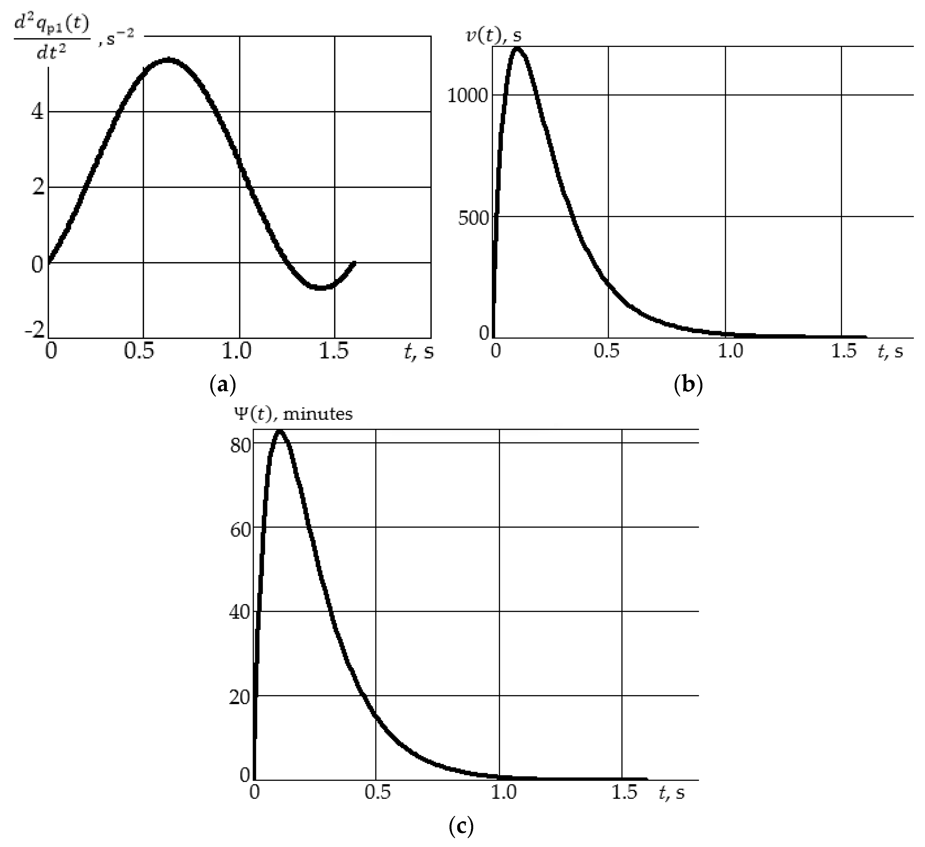
During the programmed partial movement of the robot, only one generalized coordinate of q_i = q_i(t) changes in time; the other coordinates keep constant values of q_k = q_k^* = const, k ≠ i. That is, for the i-th partial movement, all engines, except for the i-th, remain braked.

Partial movement is widely used in operations. The positioning process is carried out in the form of sequential partial movements (at first, the rotation of the first link occurs, and then, at the end of this rotation, the translational movement of the second link, and in this way each link is successively set in motion, from i = 1 to i + n links, where i = 1, 2, …, n).

The task of synthesis of the i-th transmission mechanism is solved first for the i-th partial movement. One of the tasks is the maximum unloading of drive mechanisms.

Equation of partial motions. The equations of partial motions are derived from the Lagrange differential equation of motion of the II kind. All q_k (k ≠ i) coordinates are assigned some constant value q_k = q_k^* = const. The q_k^* constants are assigned from the ranges of possible values of these coordinates in such a way that the inertial loads and loads from the gravitational forces of the links on the i-th drive are maximal.

Taking into account that the components in the considered equation, which have speed multipliers of $d{q}_k/dt$ and acceleration of $d^2{q}_k/{dt}^2$, become zero, the equation of motion of the i-th partial system will have the form of

$$a_{ii}·\frac{d^2{q}_i}{{dt}^2}+{\mathrm{F}}_i\left(q_i\right)={\mathrm{Q}}_{\mathrm{p}i},$$

(20)

where a_ii is the coefficient of inertia of the system; ${\mathrm{F}}_i\left(q_i\right)$ is the generalized load caused by active forces (in translational partial motion a_ii is the mass of moving parts of the robot, $F_i$ is the constant force; during rotary motion a_ii is the moment of inertia relative to the axis of rotation of the moving part of the robot, $F_i\left(q_i\right)$ is the moment relative to the axis of rotation of active forces, which may depend on the angle of rotation of $q_{\mathrm{i}}$.

Further, since there is one degree of mobility, the index i is omitted. Let us introduce the relation connecting the speed of the drive of $d\phi /dt$ and the executive link of $dq/dt$, as well as the generalized driving force Q_p and the moment M on the drive shaft:

$$\frac{d\phi }{dt}=k_{\mathrm{p}}·\frac{dq}{dt}, {\mathrm{Q}}_{\mathrm{p}}={\eta }_{\mathrm{p}}·k_{\mathrm{p}}·\mathrm{M},$$

(21)

where ${\eta }_{\mathrm{p}}$ is the coefficient of performance; $k_{\mathrm{p}}$ is the transmission parameter:

$$k_{\mathrm{p}}=\left\{\begin{array}{c}i,-\mathrm{f}\mathrm{o}\mathrm{r} \mathrm{a} \mathrm{r}\mathrm{o}\mathrm{t}\mathrm{a}\mathrm{t}\mathrm{i}\mathrm{n}\mathrm{g} \mathrm{p}\mathrm{a}\mathrm{i}\mathrm{r}\\ \frac{i}{R},\frac{\mathrm{r}\mathrm{a}\mathrm{d}}{\mathrm{m}}-\mathrm{f}\mathrm{o}\mathrm{r} \mathrm{a} \mathrm{t}\mathrm{r}\mathrm{a}\mathrm{n}\mathrm{s}\mathrm{l}\mathrm{a}\mathrm{t}\mathrm{i}\mathrm{o}\mathrm{n}\mathrm{a}\mathrm{l} \mathrm{p}\mathrm{a}\mathrm{i}\mathrm{r}\end{array} \right.$$

(22)

Description of the control object. The control object is a partial system, the movement of which is described by Equation (20). After joining this equation of the dynamic characteristic of the drive $\tau ·\left(\raisebox{1ex}{$dM$}\!\left/ \!\raisebox{-1ex}{$dt$}\right.\right)+\mathrm{M}=r·U-S·\left(\raisebox{1ex}{$d\phi $}\!\left/ \!\raisebox{-1ex}{$dt$}\right.\right)$ and taking into account relations (21) and (22), we arrive at a system of equations of the control object

$$\begin{array}{c}a·\frac{d^{2}q}{{dt}^2}+\mathrm{F}\left(q\right)={\eta }_{\mathrm{p}}·k_{\mathrm{p}}·\mathrm{M} \\ \tau ·\frac{d\mathrm{M}}{dt}+\mathrm{M}=r·U-S·k_{\mathrm{p}}·\frac{dq}{dt}=r·U-S·\frac{d\phi }{dt}\end{array} ,$$

(23)

where τ is the operating time of the drive, s; r is the power characteristic of the drive, H · m/V; S is the dynamic characteristic of the drive, H · m · s.

In Equation (23), the variable is the movement of the link q, the controlling action is the U voltage, which is applied to the electric drive.

Synthesis of the control law. The program control of U(t) was chosen from the condition of ideal characteristics of the drive motor:

$$U(t)=\frac{S}{r}·\frac{d\phi \left(t\right)}{dt}=\frac{S}{r}·k_{\mathrm{p}}·\frac{dq\left(t\right)}{dt}.$$

(24)

Equation of dynamic errors.

The positioning error was set as

$$\mathsf{\Psi }=q-q_{\mathrm{p}}\left(t\right),$$

(25)

where $q_{\mathrm{p}}\left(t\right)$ is the the actual movement of the link during time t.

The speed error was given as

$$v=\frac{d\mathsf{\Psi }}{dt}=\frac{dq}{dt}-\frac{d{q}_{\mathrm{p}}(t)}{dt}.$$

(26)

After substituting the control law of (24) and the relation of $q=q_{\mathrm{p}}+\mathsf{\Psi }$ into the control Equation of (23), we obtain a system of differential equations for the Ψ error positioning

$$\begin{array}{c}a·\left(\frac{d^2{q}_{\mathrm{p}}(t)}{d{t}^2}+\frac{d^2\mathsf{\Psi }}{d{t}^2}\right)+\mathrm{F}(q_{\mathrm{p}}+\mathsf{\Psi })={\eta }_{\mathrm{p}}·k_{\mathrm{p}}·\mathrm{M} \\ \tau ·\frac{d\mathrm{M}}{dt}+\mathrm{M}=-S·k_{\mathrm{p}}·\frac{dq}{dt}\end{array}.$$

(27)

After reducing the system of differential Equation (27) to one differential equation and simplifying, we obtain:

$$\tau {\tau }_{\mathrm{M}}\frac{d^3\mathsf{\Psi }}{d{t}^3}+{\tau }_{\mathrm{M}}\frac{d^2\mathsf{\Psi }}{d{t}^2}+\frac{d\mathsf{\Psi }}{dt}=-\tau {\tau }_{\mathrm{M}}\frac{d^3{q}_{\mathrm{p}}}{d{t}^3}-{\tau }_{\mathrm{M}}\frac{d^2{q}_{\mathrm{p}}}{d{t}^2}$$

$$-\frac{1}{S^{*}}\left[\tau \left(\frac{d{\mathrm{F}}_{\mathrm{p}}}{dt}+\frac{d{\mathrm{F}}_{\mathrm{p}}^{\prime }}{dt}\mathsf{\Psi }+{\mathrm{F}}_{\mathrm{p}}^{\prime }\frac{d\mathsf{\Psi }}{dt}\right)+{\mathrm{F}}_{\mathrm{p}}+{\mathrm{F}}_{\mathrm{p}}^{\prime }\mathsf{\Psi }\right],$$

(28)

where ${\mathrm{F}}_{\mathrm{p}}=\mathrm{F}(q_{\mathrm{p}}); {\mathrm{F}}_{\mathrm{p}}^{\prime }=d\mathrm{F}/d{q}_{\mathrm{p}}$; $S^{\mathrm{*}}={\eta }_{\mathrm{p}}·k_{\mathrm{p}}^2·S$; ${\tau }_{\mathrm{M}}$ is the time constant of the system of ${\tau }_{\mathrm{M}}=a/S^{\mathrm{*}}$.

After taking into account the 1/S^* parameter as small and $d\mathsf{\Psi }/dt=v$—the speed error from (28) we obtain the approximate equation

$$\tau {\tau }_{\mathrm{M}}\frac{d^{2}v}{d{t}^2}+{\tau }_{\mathrm{M}}\frac{dv}{dt}+v=-\tau {\tau }_{\mathrm{M}}\frac{d^3{q}_{\mathrm{p}}}{d{t}^3}-{\tau }_{\mathrm{M}}\frac{d^2{q}_{\mathrm{p}}}{d{t}^2} .$$

(29)

Modeling of dynamic errors. To solve Equation (29), let us assume a sinusoidal law of software acceleration change

$$\frac{d^2{q}_{\mathrm{p}}(t)}{d{t}^2}=\epsilon ·\sin \left(\mathsf{\Omega }·t\right), \mathsf{\Omega }=2·p/t_{\mathrm{p}}$$

(30)

Then, the differential of dependence (30) will be

$$\frac{d^3{q}_{\mathrm{p}}(t)}{d{t}^3}=\epsilon ·\mathsf{\Omega }·\cos \left(\mathsf{\Omega }·t\right).$$

(31)

After substituting the value of the differentials (30) and (31) into the differential Equation (29), we obtain the differential equation

$$\tau {\tau }_{\mathrm{M}}\frac{d^{2}v}{d{t}^2}+{\tau }_{\mathrm{M}}\frac{dv}{dt}+v=-\tau {·\tau }_{\mathrm{M}}·\epsilon ·\mathsf{\Omega }·\cos \left(\mathsf{\Omega }·t\right)-{\tau }_{\mathrm{M}}·\epsilon ·\sin \left(\mathsf{\Omega }·t\right).$$

(32)

We will solve the differential Equation (32) in the form of the sum of two decisions:

$$v\left(t\right)=\tilde{v}\left(t\right)+\widetilde{\stackrel{~}{v}}\left(t\right),$$

(33)

where

$$\tilde{v}\left(t\right)\equiv \tau {\tau }_{\mathrm{M}}\frac{d^{2}v}{d{t}^2}+{\tau }_{\mathrm{M}}\frac{dv}{dt}+v ;$$

(34)

$$\widetilde{\stackrel{~}{v}}\left(t\right)\equiv -\tau {·\tau }_{\mathrm{M}}·\epsilon ·\mathsf{\Omega }·\cos \left(\mathsf{\Omega }·t\right)-{\tau }_{\mathrm{M}}·\epsilon ·\sin \left(\mathsf{\Omega }·t\right).$$

(35)

We equate the differential Equation (34) to zero and replace the $v={\mathrm{e}}^{\lambda ·t}$ variable. After analytically solving the differential equations by analogy of [43,44,45], we will have:

$$\frac{d}{dt}\left({\mathrm{e}}^{\lambda ·t}\right)=\lambda ·{\mathrm{e}}^{\lambda ·t}, \frac{d^2}{d{t}^2}\left({\mathrm{e}}^{\lambda ·t}\right)={\lambda }^2·{\mathrm{e}}^{\lambda ·t} .$$

(36)

Then the differential Equation of (34) will take the form:

$$\left(\tau {·\tau }_{\mathrm{M}}·{\lambda }^2+{\tau }_{\mathrm{M}}·\lambda +1\right)·{\mathrm{e}}^{\lambda ·t}=0 .$$

(37)

Since ${\mathrm{e}}^{\lambda ·t}\ne 0$, then for any finite value of the number $\lambda$ we obtain a quadratic polynomial (38)

$$\tau {·\tau }_{\mathrm{M}}·{\lambda }^2+{\tau }_{\mathrm{M}}·\lambda +1=0,$$

(38)

whose solution will be the roots

$$\lambda =-\frac{{\tau }_{\mathrm{M}}+\sqrt{{\tau }_{\mathrm{M}}^2-4·\tau ·{\tau }_{\mathrm{M}}}}{2·\tau ·{\tau }_{\mathrm{M}}} \mathrm{a}\mathrm{n}\mathrm{d} \lambda =-\frac{{\tau }_{\mathrm{M}}-\sqrt{{\tau }_{\mathrm{M}}^2-4·\tau ·{\tau }_{\mathrm{M}}}}{2·\tau ·{\tau }_{\mathrm{M}}} .$$

(39)

The values of the roots (39) of the quadratic polynomial (38) give the solution of the differential Equation (34)

$$\tilde{v}\left(t\right)={\mathrm{B}}_1·{\mathrm{e}}^{-\frac{t·\left({\tau }_{\mathrm{M}}+\sqrt{{\tau }_{\mathrm{M}}^2-4·\tau ·{\tau }_{\mathrm{M}}}\right)}{2·\tau ·{\tau }_{\mathrm{M}}}}+{\mathrm{B}}_2·{\mathrm{e}}^{-\frac{t·\left({\tau }_{\mathrm{M}}-\sqrt{{\tau }_{\mathrm{M}}^2-4·\tau ·{\tau }_{\mathrm{M}}}\right)}{2·\tau ·{\tau }_{\mathrm{M}}}} .$$

(40)

After obtaining the general solution of the differential Equation (32), we determine the constants of integration B₁ and B₂.

Equation (35) is solved by the method of undetermined coefficients. Let us rewrite this equation as follows:

$$\widetilde{\stackrel{~}{v}}\left(t\right)={\mathrm{a}}_1·\sin \left(\mathsf{\Omega }·t\right)+{\mathrm{a}}_2·\cos \left(\mathsf{\Omega }·t\right).$$

(41)

We differentiate the equation alternately (41):

$$\frac{d\widetilde{\stackrel{~}{v}}\left(t\right)}{dt}=\mathsf{\Omega }·{\mathrm{a}}_1·\cos \left(\mathsf{\Omega }·t\right)-\mathsf{\Omega }·{\mathrm{a}}_2·\sin \left(\mathsf{\Omega }·t\right),$$

(42)

$$\frac{d^2\widetilde{\stackrel{~}{v}}\left(t\right)}{d{t}^2}=-{\mathsf{\Omega }}^2·{\mathrm{a}}_1·\sin \left(\mathsf{\Omega }·t\right)-{\mathsf{\Omega }}^2·{\mathrm{a}}_2·\cos \left(\mathsf{\Omega }·t\right).$$

(43)

Taking into account Equations (41)–(43), we will substitute in Equation (32) and accordingly obtain:

$$\tau {\tau }_{\mathrm{M}}\left(-{\mathsf{\Omega }}^2·{\mathrm{a}}_1·\sin \left(\mathsf{\Omega }·t\right)-{\mathsf{\Omega }}^2·{\mathrm{a}}_2·\cos \left(\mathsf{\Omega }·t\right)\right)+{\tau }_{\mathrm{M}}\left(\mathsf{\Omega }·{\mathrm{a}}_1·\cos \left(\mathsf{\Omega }·t\right)-\mathsf{\Omega }·{\mathrm{a}}_2·\sin \left(\mathsf{\Omega }·t\right)\right)$$

$$+{\mathrm{a}}_1·\sin \left(\mathsf{\Omega }·t\right)+{\mathrm{a}}_2·\cos \left(\mathsf{\Omega }·t\right)=-\tau {·\tau }_{\mathrm{M}}·\epsilon ·\mathsf{\Omega }·\cos \left(\mathsf{\Omega }·t\right)-{\tau }_{\mathrm{M}}·\epsilon ·\sin \left(\mathsf{\Omega }·t\right).$$

(44)

Let us simplify Equation (44)

$$\left({\tau }_{\mathrm{M}}·\mathsf{\Omega }·{\mathrm{a}}_1+{\mathrm{a}}_2-\tau ·{\tau }_{\mathrm{M}}·{\mathsf{\Omega }}^2·{\mathrm{a}}_2\right)·\cos \left(\mathsf{\Omega }·t\right)+\left({\mathrm{a}}_1-\tau ·{\tau }_{\mathrm{M}}·{\mathsf{\Omega }}^2·{\mathrm{a}}_1-{\tau }_{\mathrm{M}}·\mathsf{\Omega }·{\mathrm{a}}_2\right)·\sin \left(\mathsf{\Omega }·t\right)$$

$$-\tau {·\tau }_{\mathrm{M}}·\epsilon ·\mathsf{\Omega }·\cos \left(\mathsf{\Omega }·t\right)-{\tau }_{\mathrm{M}}·\epsilon ·\sin \left(\mathsf{\Omega }·t\right).$$

(45)

By equating the coefficients near the corresponding trigonometric functions on both sides of Equation (45), we will obtain a system of equations for determining the coefficients of a₁ and a₂:

$$\begin{array}{c}{\tau }_{\mathrm{M}}·\mathsf{\Omega }·{\mathrm{a}}_1+{\mathrm{a}}_2-\tau ·{\tau }_{\mathrm{M}}·{\mathsf{\Omega }}^2·{\mathrm{a}}_2=-\tau {·\tau }_{\mathrm{M}}·\epsilon ·\mathsf{\Omega }\\ {\mathrm{a}}_1-\tau ·{\tau }_{\mathrm{M}}·{\mathsf{\Omega }}^2·{\mathrm{a}}_1-{\tau }_{\mathrm{M}}·\mathsf{\Omega }·{\mathrm{a}}_2=-{\tau }_{\mathrm{M}}·\epsilon \end{array} .$$

(46)

After solving the system of Equation (46), we obtain

$${\mathrm{a}}_1=-\frac{{\tau }_{\mathrm{M}}\epsilon }{{\left(\tau {\tau }_{\mathrm{M}}\right)}^2{\mathsf{\Omega }}^4-2\tau {\tau }_{\mathrm{M}}{\mathsf{\Omega }}^2+{{\tau }_{\mathrm{M}}}^2{\mathsf{\Omega }}^2+1} ;$$

(47)

$${\mathrm{a}}_2=-\frac{\tau {\tau }_{\mathrm{M}}\epsilon \mathsf{\Omega }-{\left(\tau {\tau }_{\mathrm{M}}\right)}^2\epsilon {\mathsf{\Omega }}^3-{{\tau }_{\mathrm{M}}}^2\epsilon \mathsf{\Omega }}{{\left(\tau {\tau }_{\mathrm{M}}\right)}^2{\mathsf{\Omega }}^4-2\tau {\tau }_{\mathrm{M}}{\mathsf{\Omega }}^2+{{\tau }_{\mathrm{M}}}^2{\mathsf{\Omega }}^2+1} .$$

(48)

In Equation (41), we replace the coefficients a₁ and a₂ from the expressions of (47) and (48)

$$\widetilde{\stackrel{~}{v}}\left(t\right)=-\frac{\tau {\tau }_{\mathrm{M}}\epsilon \mathsf{\Omega }·\cos \left(\mathsf{\Omega }·t\right)}{{\left(\tau {\tau }_{\mathrm{M}}\right)}^2{\mathsf{\Omega }}^4-2\tau {\tau }_{\mathrm{M}}{\mathsf{\Omega }}^2+{{\tau }_{\mathrm{M}}}^2{\mathsf{\Omega }}^2+1}+\frac{{\left(\tau {\tau }_{\mathrm{M}}\right)}^2\epsilon {\mathsf{\Omega }}^3·\cos \left(\mathsf{\Omega }·t\right)}{{\left(\tau {\tau }_{\mathrm{M}}\right)}^2{\mathsf{\Omega }}^4-2\tau {\tau }_{\mathrm{M}}{\mathsf{\Omega }}^2+{{\tau }_{\mathrm{M}}}^2{\mathsf{\Omega }}^2+1}$$

$$+\frac{{{\tau }_{\mathrm{M}}}^2\epsilon \mathsf{\Omega }·\cos \left(\mathsf{\Omega }·t\right)}{{\left(\tau {\tau }_{\mathrm{M}}\right)}^2{\mathsf{\Omega }}^4-2\tau {\tau }_{\mathrm{M}}{\mathsf{\Omega }}^2+{{\tau }_{\mathrm{M}}}^2{\mathsf{\Omega }}^2+1}-\frac{{\tau }_{\mathrm{M}}\epsilon ·\sin \left(\mathsf{\Omega }·t\right)}{{\left(\tau {\tau }_{\mathrm{M}}\right)}^2{\mathsf{\Omega }}^4-2\tau {\tau }_{\mathrm{M}}{\mathsf{\Omega }}^2+{{\tau }_{\mathrm{M}}}^2{\mathsf{\Omega }}^2+1} .$$

(49)

The general solution of the differential Equation (32) for determining the speed error is as follows:

$$v\left(t\right)={\mathrm{B}}_1·{\mathrm{e}}^{-\frac{t·\left({\tau }_{\mathrm{M}}+\sqrt{{\tau }_{\mathrm{M}}^2-4·\tau ·{\tau }_{\mathrm{M}}}\right)}{2·\tau ·{\tau }_{\mathrm{M}}}}+{\mathrm{B}}_2·{\mathrm{e}}^{-\frac{t·\left({\tau }_{\mathrm{M}}-\sqrt{{\tau }_{\mathrm{M}}^2-4·\tau ·{\tau }_{\mathrm{M}}}\right)}{2·\tau ·{\tau }_{\mathrm{M}}}}$$

$$+\frac{\left({{\tau }_{\mathrm{M}}}^2\epsilon \mathsf{\Omega }+{\left(\tau {\tau }_{\mathrm{M}}\right)}^2\epsilon {\mathsf{\Omega }}^3-\tau {\tau }_{\mathrm{M}}\epsilon \mathsf{\Omega }\right)\cos \left(\mathsf{\Omega }·t\right)}{{\left(\tau {\tau }_{\mathrm{M}}\right)}^2{\mathsf{\Omega }}^4-2\tau {\tau }_{\mathrm{M}}{\mathsf{\Omega }}^2+{{\tau }_{\mathrm{M}}}^2{\mathsf{\Omega }}^2+1}-\frac{{\tau }_{\mathrm{M}}\epsilon ·\sin \left(\mathsf{\Omega }·t\right)}{{\left(\tau {\tau }_{\mathrm{M}}\right)}^2{\mathsf{\Omega }}^4-2\tau {\tau }_{\mathrm{M}}{\mathsf{\Omega }}^2+{{\tau }_{\mathrm{M}}}^2{\mathsf{\Omega }}^2+1} .$$

(50)

We determine the integration constants B₁ and B₂ under specific conditions of operation of the robot manipulator. At the moment of time t = 0, the speed and acceleration of the manipulator link of the robot will be equal to zero. Under this condition we define constants of integration:

• for the speed

  $$0={\mathrm{B}}_1+{\mathrm{B}}_2+\frac{\left({{\tau }_{\mathrm{M}}}^2\epsilon \mathsf{\Omega }+{\left(\tau {\tau }_{\mathrm{M}}\right)}^2\epsilon {\mathsf{\Omega }}^3-\tau {\tau }_{\mathrm{M}}\epsilon \mathsf{\Omega }\right)}{{\left(\tau {\tau }_{\mathrm{M}}\right)}^2{\mathsf{\Omega }}^4-2\tau {\tau }_{\mathrm{M}}{\mathsf{\Omega }}^2+{{\tau }_{\mathrm{M}}}^2{\mathsf{\Omega }}^2+1} ,$$

  (51)

  for the acceleration we will differentiate Equation (50)

  $$\frac{dv\left(t\right)}{dt}=-{\mathrm{B}}_1·\frac{\left({\tau }_{\mathrm{M}}+\sqrt{{\tau }_{\mathrm{M}}^2-4·\tau ·{\tau }_{\mathrm{M}}}\right)}{2·\tau ·{\tau }_{\mathrm{M}}}·{\mathrm{e}}^{-\frac{t·\left({\tau }_{\mathrm{M}}+\sqrt{{\tau }_{\mathrm{M}}^2-4·\tau ·{\tau }_{\mathrm{M}}}\right)}{2·\tau ·{\tau }_{\mathrm{M}}}}$$

  $${-\mathrm{B}}_2·\frac{\left({\tau }_{\mathrm{M}}-\sqrt{{\tau }_{\mathrm{M}}^2-4·\tau ·{\tau }_{\mathrm{M}}}\right)}{2·\tau ·{\tau }_{\mathrm{M}}}·{\mathrm{e}}^{-\frac{t·\left({\tau }_{\mathrm{M}}-\sqrt{{\tau }_{\mathrm{M}}^2-4·\tau ·{\tau }_{\mathrm{M}}}\right)}{2·\tau ·{\tau }_{\mathrm{M}}}}$$

  $$-\frac{\mathsf{\Omega }\left({{\tau }_{\mathrm{M}}}^2\epsilon \mathsf{\Omega }+{\left(\tau {\tau }_{\mathrm{M}}\right)}^2\epsilon {\mathsf{\Omega }}^3-\tau {\tau }_{\mathrm{M}}\epsilon \mathsf{\Omega }\right)\sin \left(\mathsf{\Omega }·t\right)}{{\left(\tau {\tau }_{\mathrm{M}}\right)}^2{\mathsf{\Omega }}^4-2\tau {\tau }_{\mathrm{M}}{\mathsf{\Omega }}^2+{{\tau }_{\mathrm{M}}}^2{\mathsf{\Omega }}^2+1}-\frac{\mathsf{\Omega }{\tau }_{\mathrm{M}}\epsilon ·\cos \left(\mathsf{\Omega }·t\right)}{{\left(\tau {\tau }_{\mathrm{M}}\right)}^2{\mathsf{\Omega }}^4-2\tau {\tau }_{\mathrm{M}}{\mathsf{\Omega }}^2+{{\tau }_{\mathrm{M}}}^2{\mathsf{\Omega }}^2+1} .$$

  (52)

To determine the acceleration, we substitute t = 0 in Equation (52) and obtain the expression for the integration constants:

$$0=-{\mathrm{B}}_1·\frac{\left({\tau }_{\mathrm{M}}+\sqrt{{\tau }_{\mathrm{M}}^2-4·\tau ·{\tau }_{\mathrm{M}}}\right)}{2·\tau ·{\tau }_{\mathrm{M}}}{-\mathrm{B}}_2·\frac{\left({\tau }_{\mathrm{M}}-\sqrt{{\tau }_{\mathrm{M}}^2-4·\tau ·{\tau }_{\mathrm{M}}}\right)}{2·\tau ·{\tau }_{\mathrm{M}}}$$

$$-\frac{\mathsf{\Omega }{\tau }_{\mathrm{M}}\epsilon }{{\left(\tau {\tau }_{\mathrm{M}}\right)}^2{\mathsf{\Omega }}^4-2\tau {\tau }_{\mathrm{M}}{\mathsf{\Omega }}^2+{{\tau }_{\mathrm{M}}}^2{\mathsf{\Omega }}^2+1} .$$

(53)

Considering expressions of (51) and (53) also t = 0 and t = 1.6 s, also data ($\tau =0.05 \mathrm{s}, {\tau }_{\mathrm{M}}=0.025 \mathrm{s})$, we determine the constants of integration:

$${\mathrm{B}}_1=-\left(\frac{0.489}{9.119·{10}^{-11}}-\frac{\mathsf{\Omega }{\tau }_{\mathrm{M}}\epsilon \left({\tau }_{\mathrm{M}}+{{\tau }_{\mathrm{M}}\tau }^2{\mathsf{\Omega }}^2-\tau \right)}{{\left(\tau {\tau }_{\mathrm{M}}\right)}^2{\mathsf{\Omega }}^4-2\tau {\tau }_{\mathrm{M}}{\mathsf{\Omega }}^2+{{\tau }_{\mathrm{M}}}^2{\mathsf{\Omega }}^2+1}\right)$$

$$\times \frac{1.389}{9.119·{10}^{-7}-1.389}-\frac{0.489}{9.119\cdot {10}^{-11}} ,$$

(54)

$${\mathrm{B}}_2=\left(\frac{0.489}{9.119·{10}^{-11}}-\frac{\mathsf{\Omega }{\tau }_{\mathrm{M}}\epsilon \left({\tau }_{\mathrm{M}}+{{\tau }_{\mathrm{M}}\tau }^2{\mathsf{\Omega }}^2-\tau \right)}{{\left(\tau {\tau }_{\mathrm{M}}\right)}^2{\mathsf{\Omega }}^4-2\tau {\tau }_{\mathrm{M}}{\mathsf{\Omega }}^2+{{\tau }_{\mathrm{M}}}^2{\mathsf{\Omega }}^2+1}\right)·\frac{9.119·{10}^{-7}}{9.119·{10}^{-7}-1.389} .$$

(55)

The positioning error is determined by the integral

$$\mathsf{\Psi }\left(t\right)=\underset{0}{\overset{t}{\int }}v\left(t\right)dt,$$

$$\mathsf{\Psi }\left(t\right)={-\mathrm{B}}_1·\frac{2\tau {\tau }_{\mathrm{M}}}{{\tau }_{\mathrm{M}}+\sqrt{{\tau }_{\mathrm{M}}^2-4\tau {\tau }_{\mathrm{M}}}}\left(1-\frac{1}{{\mathrm{e}}^{\frac{t·\left(-{\tau }_{\mathrm{M}}-\sqrt{{\tau }_{\mathrm{M}}^2-4·\tau ·{\tau }_{\mathrm{M}}}\right)}{2·\tau ·{\tau }_{\mathrm{M}}}}}\right)$$

$$-{\mathrm{B}}_2·\frac{2\tau {\tau }_{\mathrm{M}}}{{\tau }_{\mathrm{M}}-\sqrt{{\tau }_{\mathrm{M}}^2-4\tau {\tau }_{\mathrm{M}}}}\left(1-\frac{1}{{\mathrm{e}}^{\frac{t·\left(-{\tau }_{\mathrm{M}}+\sqrt{{\tau }_{\mathrm{M}}^2-4·\tau ·{\tau }_{\mathrm{M}}}\right)}{2·\tau ·{\tau }_{\mathrm{M}}}}}\right)$$

$$+\frac{\left({{\tau }_{\mathrm{M}}}^2\epsilon +{\left(\tau {\tau }_{\mathrm{M}}\right)}^2\epsilon {\mathsf{\Omega }}^2-\tau {\tau }_{\mathrm{M}}\epsilon \right)\sin \left(\mathsf{\Omega }·t\right)}{{\left(\tau {\tau }_{\mathrm{M}}\right)}^2{\mathsf{\Omega }}^4-2\tau {\tau }_{\mathrm{M}}{\mathsf{\Omega }}^2+{{\tau }_{\mathrm{M}}}^2{\mathsf{\Omega }}^2+1}+\frac{{\tau }_{\mathrm{M}}\epsilon ·\left(\cos \left(\mathsf{\Omega }·t\right)-1\right)}{\mathsf{\Omega }\left({\left(\tau {\tau }_{\mathrm{M}}\right)}^2{\mathsf{\Omega }}^4-2\tau {\tau }_{\mathrm{M}}{\mathsf{\Omega }}^2+{{\tau }_{\mathrm{M}}}^2{\mathsf{\Omega }}^2+1\right)} .$$

(56)

The dynamic error was modeled under the condition of a sinusoidal law of changes in the programmed acceleration. The analytical solution of the differential Equation (50) makes it possible to program the movement speed of the robot gripper for given time parameters. The integration constants B₁ and B₂ were determined under the specific conditions of operation of the robot manipulator. At the moment of time t = 0 and after the end of the movement, the speed and acceleration of the manipulator link of the robot will be zero. Let the maximum time of the movement of the robot gripper be t = 1.6 s. The constants B₁ and B₂ for a specific length of time for moving the catcher will have their dependencies.

So, for the duration of the movement of the catcher t = 1.6 s, we obtained the speed Equation (50) of the movement of the catcher, the acceleration Equation (52) of the movement of the catcher, and the equation of the positioning error (56). Constant integrations B₁ (54) and B₂ (55) are calculated for the duration of the robot gripper movement t = 1.6 s.

3. Results and Discussion

The following restrictions are adopted for modeling the positioning error of the manipulator. There is no flexibility in the connections and links and, accordingly, there are no high-frequency oscillations of the links. The mass of the links of the robot manipulator in relation to the mass of the object being moved is on average 100 or more times higher than the mass of the object being moved.

3.1. Modeling of the Position and Orientation Error of the Robot Gripper Due to the Temperature Deformation of the Manipulator Links

We will simulate the position and orientation error of the robot gripper due to temperature deformations of the third link for the manipulator scheme shown in Figure 3.

To take into account the temperature deformations of the third link, we introduce an additional fourth local system of axes of O₄x₄y₄z₄, combining the origin of O₄ with the pole M of the gripper. Let us set the following parameters of the manipulator: l₂ = 1 m; l_3y = l_3z = 0.5 m; q₁₀ = q₃₀ = 0; q₂₀ = 0.1 m; ∆q₁ = ∆q₃ = 0.001 rad; ∆q₂ = 10⁻⁴ m; ∆t = +20 °C.

For the initial position of the manipulator, in which the angular coordinates q₁ = q₃ = 0, all rotation matrices are unitary, i.e.,

A_0,1 = A_1,2 = A_2,3 = A_0,2 = A_0,3 = I = diag[1, 1, 1],

(57)

and we also have

$$r_{\mathrm{M}}^{\left(3\right)}=\left[\begin{array}{c}0\\ l_{3\mathrm{y}}\\ l_{3\mathrm{z}}\end{array}\right]=\left[\begin{array}{c}0\\ 0.5\\ 0.5\end{array}\right], r_{\mathrm{M}}^{\left(2\right)}=\left[\begin{array}{c}0\\ l_{3\mathrm{y}}+l_2\\ l_{3\mathrm{z}}\end{array}\right]=\left[\begin{array}{c}0\\ 1.5\\ 0.5\end{array}\right], r_{\mathrm{M}}^{\left(1\right)}=\left[\begin{array}{c}0\\ l_{3\mathrm{y}}+l_2\\ l_{3\mathrm{z}}+q_{20}\end{array}\right]=\left[\begin{array}{c}0\\ 1.5\\ 0.6\end{array}\right], \mathrm{m}.$$

From the kinematic scheme (Figure 3), we determine the vectors of a small linear displacement of the O_i point at the fixed point of O_i−1 (i = 4, 3, 2, 1):

$${\xi }_4^{\left(4\right)}={\left[0; \alpha ·l_{3y}·∆t; \alpha ·l_{3z}·∆t\right]}^{\mathrm{T}}={\left[0; 1.2; 1.2\right]}^{\mathrm{T}}·{10}^{-4} \mathrm{m};$$

$${\xi }_3^{\left(3\right)}={\left[0; \alpha ·l_2·∆t; 0\right]}^{\mathrm{T}}={\left[0; 2.4; 0\right]}^{\mathrm{T}}·{10}^{-4} \mathrm{m};$$

(58)

$${\xi }_2^{\left(2\right)}={\left[0; 0; \alpha ·q_{20}·∆t+∆q_2\right]}^{\mathrm{T}}={\left[0; 0; 1.24\right]}^{\mathrm{T}}·{10}^{-4} \mathrm{m};$$

$${\xi }_1^{\left(1\right)}={\left[0; 0; 0\right]}^{\mathrm{T}}.$$

From the same scheme, we determine the vectors of small rotations of ${\vartheta }_i^{\left(i\right)}$. After taking into account that the rotation axis of $∆q_1$ is x₁, and the rotation of $∆q_3$ is the z₃ axis, we obtain

$${\vartheta }_1^{\left(1\right)}={\left[∆q_1; 0; 0\right]}^{\mathrm{T}}, {\vartheta }_3^{\left(3\right)}={\left[0; 0; ∆q_3\right]}^{\mathrm{T}}, {\vartheta }_2^{\left(2\right)}={\vartheta }_4^{\left(4\right)}={\left[0; 0; 0\right]}^{\mathrm{T}}.$$

(59)

We form a skew symmetric matrix of small turns by (3):

$${\mathsf{\Theta }}_1=\left[\begin{array}{ccc}0& 0& 0\\ 0& 0& -∆q_1\\ 0& ∆q_1& 0\end{array}\right], {\mathsf{\Theta }}_3=\left[\begin{array}{ccc}0& -∆q_3& 0\\ ∆q_3& 0& 0\\ 0& 0& 0\end{array}\right], {\mathsf{\Theta }}_2={\mathsf{\Theta }}_4=0 .$$

We determine the linear errors of the position of the gripper pole in the reference system of the axes according to (1):

$$∆r_{\mathrm{M}1}^{\left(0\right)}={\mathrm{A}}_{\mathrm{0,1}}\left({\mathsf{\Theta }}_1{r}_{\mathrm{M}}^{\left(1\right)}+{\xi }_1^{\left(1\right)}\right)={\mathsf{\Theta }}_1{r}_{\mathrm{M}}^{\left(1\right)}=\left[\begin{array}{ccc}0& 0& 0\\ 0& 0& -0.001\\ 0& 0.001& 0\end{array}\right]\left[\begin{array}{c}0\\ 1.5\\ 0.6\end{array}\right]=\left[\begin{array}{c}0\\ -0.6\\ 1.5\end{array}\right] \mathrm{mm},$$

$$∆r_{\mathrm{M}2}^{\left(0\right)}={\mathrm{A}}_{\mathrm{0,2}}\left({\mathsf{\Theta }}_2{r}_{\mathrm{M}}^{\left(2\right)}+{\xi }_2^{\left(2\right)}\right)={\xi }_2^{\left(2\right)}=\left[\begin{array}{c}0\\ 0\\ 0.124\end{array}\right] \mathrm{mm},$$

$$∆r_{\mathrm{M}3}^{\left(0\right)}={\mathrm{A}}_{\mathrm{0,3}}\left({\mathsf{\Theta }}_3{r}_{\mathrm{M}}^{\left(3\right)}+{\xi }_3^{\left(3\right)}\right)=\left[\begin{array}{ccc}0& -0.001& 0\\ 0.001& 0& 0\\ 0& 0& 0\end{array}\right]\left[\begin{array}{c}0\\ 0.5\\ 0.5\end{array}\right]+\left[\begin{array}{c}0\\ 2.4\\ 0\end{array}\right]·{10}^{-4}=\left[\begin{array}{c}-0.5\\ 0.24\\ 0\end{array}\right] \mathrm{mm},$$

$$∆r_{\mathrm{M}4}^{\left(0\right)}={\mathrm{A}}_{\mathrm{0,4}}\left({\mathsf{\Theta }}_4{r}_{\mathrm{M}}^{\left(4\right)}+{\xi }_4^{\left(4\right)}\right)={\xi }_4^{\left(4\right)}=\left[\begin{array}{c}0\\ 0.12\\ 0.12\end{array}\right] \mathrm{mm}.$$

The total linear error of the position of the gripper is a column vector of

$${\vartheta }^{\left(0\right)}=\sum _{\mathrm{i}=1}^4{\mathrm{A}}_{0,\mathrm{i}}·{\vartheta }_{\mathrm{i}}^{\left(\mathrm{i}\right)}={\vartheta }_1^{\left(1\right)}+{\vartheta }_3^{\left(3\right)}=\left[\begin{array}{c}0.001\\ 0\\ 0.001\end{array}\right]=\left[\begin{array}{c}{\vartheta }_{\mathrm{x}}^{\left(0\right)}\\ {\vartheta }_{\mathrm{y}}^{\left(0\right)}\\ {\vartheta }_{\mathrm{z}}^{\left(0\right)}\end{array}\right].$$

3.2. Modeling of Static Deformations and Manipulator Errors under Elastic Pliability of Robot Links

We will perform simulation of static deformations and errors of the manipulator. For example, consider the kinematic scheme of the elastic robot manipulator in the initial position (Figure 4). The elastic pliability of drives of kinematic pairs is modeled by elastic elements that have stiffness of c₁, c₂, and c₃. The gripper is loaded with technological loads of ${\mathrm{F}}_{\mathrm{x}}, {\mathrm{F}}_{\mathrm{y}}, {\mathrm{F}}_{\mathrm{z}},$ and moments of ${\mathrm{M}}_x, {\mathrm{M}}_y, {\mathrm{M}}_z$.

We set arbitrary parameters of the manipulator elements for modeling deformations and errors. We accept the following: l₂ = 1 m; l_3y = l_3z = 0.5 m; q₁₀ = q₃₀ = 0; q₂₀ = 0.1 m; e₁ = e₃ = e_ang = 2 ∙ 10⁻⁶ rad/N∙m; C₁ = C₂ = 1/e_ang = 0.5 ∙ 10⁶ N∙m/rad; e₂ = e_lin = 4 ∙ 10⁻⁶ m/N, C₂ = 1/e_lin = 0.25 ∙ 10⁶ N∙m/rad; G = 200 N; b = 0.5 m.

Other data necessary for modeling were obtained from the results of modeling the position and orientation error of the robot gripper due to the temperature deformation of the manipulator links:

A_0,1 = A_1,2 = A_2,3 = I = diag[1, 1, 1],

$$r_{\mathrm{M}}^{\left(3\right)}=\left[\begin{array}{c}0\\ 0.5\\ 0.5\end{array}\right], r_{\mathrm{M}}^{\left(2\right)}=\left[\begin{array}{c}0\\ 1.5\\ 0.5\end{array}\right], r_{\mathrm{M}}^{\left(1\right)}=\left[\begin{array}{c}0\\ 1.5\\ 0.6\end{array}\right], \mathrm{m};$$

$${\xi }_1^{\left(1\right)}={\xi }_3^{\left(3\right)}={\left[0; 0; 0\right]}^{\mathrm{T}}, {\xi }_2^{\left(2\right)}={\left[0; 0; ∆q_2\right]}^{\mathrm{T}} \mathrm{m};$$

(60)

$${\vartheta }_1^{\left(1\right)}={\left[∆q_1; 0; 0\right]}^{\mathrm{T}}, {\vartheta }_3^{\left(3\right)}={\left[0; 0; ∆q_3\right]}^{\mathrm{T}}, {\vartheta }_2^{\left(2\right)}={\vartheta }_4^{\left(4\right)}={\left[0; 0; 0\right]}^{\mathrm{T}};$$

$${\mathsf{\Theta }}_1=\left[\begin{array}{ccc}0& 0& 0\\ 0& 0& -∆q_1\\ 0& ∆q_1& 0\end{array}\right],{\mathsf{\Theta }}_2=0, {\mathsf{\Theta }}_3=\left[\begin{array}{ccc}0& -∆q_3& 0\\ ∆q_3& 0& 0\\ 0& 0& 0\end{array}\right].$$

Modeling of deformations of elastic elements $∆q_i$. We load the gripper with a unit force ${\mathrm{F}}_{\mathrm{x}}=1$ in the absence of other loads. Deformation $∆q_1=0$, because the ${\mathrm{F}}_{\mathrm{x}}$ force is parallel to the axis of rotation x₁ and its moment relative to this axis is zero. Deformation $∆q_2=0$, because the ${\mathrm{F}}_{\mathrm{x}}$ force acts perpendicular to the direction of $q_2$ movement. The deformation will be as:

$$∆q_2=-{\mathrm{F}}_{\mathrm{x}}{l}_{3\mathrm{y}}/{\mathrm{C}}_3=-1·{10}^{-6} \mathrm{r}\mathrm{a}\mathrm{d},$$

(the minus sign means that the ${\mathrm{F}}_{\mathrm{x}}$ force tries to turn the third link clockwise relative to the z₃ axis of rotation).

We load the gripper with the ${\mathrm{F}}_{\mathrm{y}}=1$ force in the absence of other loads. The deformation will be:

$$∆q_1=-{\mathrm{F}}_{\mathrm{y}}·\left(l_{3\mathrm{y}}+q_{20}\right)/{\mathrm{c}}_1=-1.2·{10}^{-6} \mathrm{r}\mathrm{a}\mathrm{d}.$$

Deformations $∆q_2=0$ and $∆q_3=0$.

After loading the gripper with a unit force ${\mathrm{F}}_{\mathrm{z}}=1$, we will have:

$$∆q_1={\mathrm{F}}_{\mathrm{z}}·(l_{3\mathrm{y}}+l_2)/{\mathrm{c}}_1=3·{10}^{-6} \mathrm{r}\mathrm{a}\mathrm{d}; ∆q_2={\mathrm{F}}_{\mathrm{z}}/{\mathrm{c}}_2=4·{10}^{-6} \mathrm{r}\mathrm{a}\mathrm{d};∆q_3=0.$$

When loading the gripper with single moments, it is necessary to take into account that arbitrary moment loading does not cause linear deformations, i.e., $∆q_2=0$. The unit moment ${\mathrm{M}}_x=1$ causes deformation only in the first kinematic pair, because it has an x₁ axis of rotation:

$$∆q_1={\mathrm{M}}_{\mathrm{x}}/{\mathrm{c}}_1=1/0.5·{10}^6=2·{10}^{-6} \mathrm{r}\mathrm{a}\mathrm{d} ;∆q_2=0 ; ∆q_3=0.$$

All three deformations from the moment ${\mathbf{M}}_{\mathbf{y}}=1$ are equal to zero, therefore $∆q_1=∆q_2=∆q_3=0$.

The unitary moment ${\mathbf{M}}_{\mathbf{z}}=1$ creates deformation only in the third kinematic pair with the z₃ axis of rotation:

$$∆q_1=∆q_2=0; ∆q_3={\mathrm{M}}_{\mathrm{z}}/{\mathrm{c}}_3=1/0.5·{10}^6=2·{10}^{-6} \mathrm{r}\mathrm{a}\mathrm{d}.$$

The results of simulation of deformations are summarized in the

Table 1. Results of elastic deformation modeling of kinematic pairs.

Deformations		${\mathit{F}}_{\mathit{x}}=1$	${\mathit{F}}_{\mathit{y}}=1$	${\mathit{F}}_{\mathit{z}}=1$	${\mathrm{M}}_{\mathit{x}}=1$	${\mathrm{M}}_{\mathit{y}}=1$	${\mathrm{M}}_{\mathit{z}}=1$
$∆q_1$	${10}^{-6} \mathrm{r}\mathrm{a}\mathrm{d}$	0	−1.2	3	2	0	0
$∆q_2$	${10}^{-6} \mathrm{r}\mathrm{a}\mathrm{d}$	0	0	4	0	0	0
$∆q_3$	${10}^{-6} \mathrm{r}\mathrm{a}\mathrm{d}$	−1	0	0	0	0	2

.

Calculation of elements of the E matrix of elastic deformations. For the calculation, we will use expressions (18) and (19), data from the table, the column number of which corresponds to the column number of the matrix E, the elements of which we are looking for. We define in the following sequence:

• Elements of the first column:

  $$∆r_{\mathrm{M}}^{\left(0\right)}({\mathrm{F}}_{\mathrm{x}})={\mathrm{A}}_{0,3}·\left({\mathsf{\Theta }}_3·r_{\mathrm{M}}^{\left(3\right)}+{\xi }_3^{\left(3\right)}\right)={\mathsf{\Theta }}_3·r_{\mathrm{M}}^{\left(3\right)}=\left[\begin{array}{ccc}0& -∆q_3& 0\\ ∆q_3& 0& 0\\ 0& 0& 0\end{array}\right]·\left[\begin{array}{c}0\\ 0.5\\ 0.5\end{array}\right]=\left[\begin{array}{c}0.5\\ 0\\ 0\end{array}\right]·{10}^{-6} \mathrm{m};$$

  $${\vartheta }^{\left(0\right)}({\mathrm{F}}_{\mathrm{x}})={\mathrm{A}}_{0,3}·{\vartheta }_3^{\left(3\right)}=\left[\begin{array}{c}0\\ 0\\ ∆q_3\end{array}\right]=\left[\begin{array}{c}0\\ 0\\ -1\end{array}\right]·{10}^{-6} \mathrm{rad};$$
• Elements of the second column:

  $$∆r_{\mathrm{M}}^{\left(0\right)}({\mathrm{F}}_{\mathrm{y}})={\mathsf{\Theta }}_1·r_{\mathrm{M}}^{\left(1\right)}=\left[\begin{array}{ccc}0& 0& 0\\ 0& 0& -∆q_1\\ 0& ∆q_1& 0\end{array}\right]·\left[\begin{array}{c}0\\ 1.5\\ 0.6\end{array}\right]=\left[\begin{array}{c}0\\ 0.72\\ -1.8\end{array}\right]·{10}^{-6} \mathrm{m};$$

  $${\vartheta }^{\left(0\right)}({\mathrm{F}}_{\mathrm{y}})={\vartheta }_1^{\left(1\right)}=\left[\begin{array}{c}∆q_1\\ 0\\ 0\end{array}\right]=\left[\begin{array}{c}-1.2\\ 0\\ 0\end{array}\right]·{10}^{-6} \mathrm{rad};$$
• Elements of the third column:

  $$∆r_{\mathrm{M}}^{\left(0\right)}({\mathrm{F}}_{\mathrm{z}})={\mathsf{\Theta }}_1·r_{\mathrm{M}}^{\left(1\right)}+{\xi }_2^{\left(2\right)}=\left[\begin{array}{ccc}0& 0& 0\\ 0& 0& -∆q_1\\ 0& ∆q_1& 0\end{array}\right]·\left[\begin{array}{c}0\\ 1.5\\ 0.6\end{array}\right]+\left[\begin{array}{c}0\\ 0\\ 0\end{array}\right]=\left[\begin{array}{c}0\\ -1.8\\ 8.5\end{array}\right]·{10}^{-6} \mathrm{m};$$

  $${\vartheta }^{\left(0\right)}({\mathrm{F}}_{\mathrm{z}})={\vartheta }_1^{\left(1\right)}=\left[\begin{array}{c}3\\ 0\\ 0\end{array}\right]·{10}^{-6}$$
• Elements of the fourth column:

  $$∆r_{\mathrm{M}}^{\left(0\right)}({\mathrm{M}}_{\mathrm{x}})={\mathsf{\Theta }}_1·r_{\mathrm{M}}^{\left(1\right)}=\left[\begin{array}{ccc}0& 0& 0\\ 0& 0& -2\\ 0& 2& 0\end{array}\right]·\left[\begin{array}{c}0\\ 1.5\\ 0.6\end{array}\right]=\left[\begin{array}{c}0\\ -1.2\\ 3\end{array}\right]·{10}^{-6} \mathrm{m};$$

  $${\vartheta }^{\left(0\right)}({\mathrm{M}}_{\mathrm{x}})={\vartheta }_1^{\left(1\right)}=\left[\begin{array}{c}2\\ 0\\ 0\end{array}\right]·{10}^{-6} \mathrm{rad};$$
• All elements of the fifth column are zero; elements of the sixth column;

  $$∆r_{\mathrm{M}}^{\left(0\right)}({\mathrm{M}}_{\mathrm{z}})={\mathsf{\Theta }}_3·r_{\mathrm{M}}^{\left(3\right)}=\left[\begin{array}{ccc}0& -2& 0\\ 2& 0& 0\\ 0& 2& 0\end{array}\right]·\left[\begin{array}{c}0\\ 0.5\\ 0.5\end{array}\right]·{10}^{-6}=\left[\begin{array}{c}-1\\ 0\\ 3\end{array}\right]·{10}^{-6} \mathrm{m};$$

  $${\vartheta }^{\left(0\right)}({\mathrm{M}}_{\mathrm{z}})={\vartheta }_3^{\left(3\right)}=\left[\begin{array}{c}0\\ 0\\ 2\end{array}\right]·{10}^{-6} \mathrm{rad}.$$

Based on the results of the calculations, we form a matrix of elastic pliability of the gripper in the initial position of the robot:

$$\mathrm{E}=\left[\begin{array}{c}\begin{array}{ccc}0.5& 0& 0\\ 0 & 0.72 & -1.8\\ 0 & -1.8& 8.5\end{array} \begin{array}{ccc}0& 0& -1\\ -1.2& 0& 0\\ 3 & 0& 0\end{array}\\ \begin{array}{ccc}0 & -1.2 & 3\\ 0 & 0& 0\\ -1& 0& 0\end{array} \begin{array}{ccc}2 & 0 & 0\\ 0 & 0 & 0\\ 0 & 0 & 2\end{array}\end{array}\right]·{10}^{-6}.$$

(61)

The matrix E has the property of symmetry and the main diagonal of the elements is positive.

Calculation of the vector of errors of the gripper position. We assume that the gripper holds a longitudinal object weighing G = 200 N, the center of gravity of the object is located at a distance of b = 0.5 m in the horizontal direction from the pole M of the gripper (Figure 2). We bring the gravitational forces G to the pole M. There will be a concentrated load of F_z = G =−200 N and moment M_x = −G∙b = −200 ∙ 0.5 = −100 N∙m. So, the column vector of loads (8) in this case has the form:

$$\mathrm{Q}={\left[0; 0;-200;-100; 0; 0 \right]}^{\mathrm{T}}.$$

(62)

Applying (11), we determine the vector of position errors of the gripper

$${\delta }_{\mathrm{M}}=\mathrm{E}·\mathrm{Q}=\left[\begin{array}{c}\begin{array}{c}0\\ 0.48\\ -2\end{array}\\ \begin{array}{c}-0.8\\ 0\\ 0\end{array}\end{array}\right]·{10}^{-3}=\left[\begin{array}{c}\begin{array}{c}∆{\mathrm{x}}_{\mathrm{M}}^{\left(0\right)}\\ ∆{\mathrm{y}}_{\mathrm{M}}^{\left(0\right)}\\ ∆{\mathrm{z}}_{\mathrm{M}}^{\left(0\right)}\end{array}\\ \begin{array}{c}{\vartheta }_{\mathrm{x}}^{\left(0\right)}\\ {\vartheta }_{\mathrm{y}}^{\left(0\right)}\\ {\vartheta }_{\mathrm{z}}^{\left(0\right)}\end{array}\end{array}\right].$$

(63)

The results of the calculation (26) show that the pole M of the gripper as a result of the loads shifted to the right by 0.48 ∙ 10⁻³ m and down by 2 ∙ 10⁻³ m. At the same time, the gripper tilted at an angle of 0.8 ∙ 10⁻³ rad clockwise around the x₀ axis.

3.3. Modeling of Dynamic Errors in the Partial System of Motion of Robot Links

The first partial system. To obtain this system, we brake the drive of the second kinematic pair in the position of $q_2=q_2^{*}=0.7 \mathrm{m}=\mathrm{c}\mathrm{o}\mathrm{n}\mathrm{s}\mathrm{t}$. Thus, the second link is distant from the x₁ axis of rotation by the maximum possible distance and, accordingly, the moments of inertial loads and loads from the gravity of the second link on the drive of the q₁ coordinate will be maximum. In the first partial movement, only one q₁ coordinate changes (Figure 5).

We compose the differential equation for the q₁ coordinate, and given that q₂ = 0.7 m, ${\dot{q}}_2=0, {\ddot{q}}_2=0$, we obtain the equation of the first partial motion

$$78.8·{\ddot{q}}_1-525·\sin q_1+340·\cos q_1={\mathrm{Q}}_{\mathrm{p}1}, \mathrm{N}·\mathrm{m}.$$

(64)

In this equation, the inertia coefficient of a₁₁ = 78.8 kg∙m² is the moment of inertia relative to the x₁ axis of rotation of both links of the robot, and the component of ${\mathrm{F}}_1\left(q_1\right)=-525·\sin q_1+340·\cos q_1$ is the moment of gravity of the links, taken with the opposite sign.

The partial system as a control object we described by Equation of (64) together with the dynamic characteristic of the drive of the first link

$$0.05·\frac{d{\mathrm{M}}_1}{dt}+{\mathrm{M}}_1=0.0773·U_1-0.135·\frac{d{\phi }_1}{dt}$$

After applying Equation (21), which, under the condition of k_p1 = i1 = 51 will have the form of

$$\frac{d\phi }{dt}=51·\frac{d{q}_1}{dt}, {\mathrm{Q}}_{\mathrm{p}}=0.9·51·{\mathrm{M}}_1=46·{\mathrm{M}}_1,$$

(65)

we obtain the equation of the control object

$$\begin{array}{c}78.8·\frac{d^2{q}_1}{{dt}^2}-525·\sin q_1+340·\cos q_1=46·{\mathrm{M}}_1\\ 0.05·\frac{d{\mathrm{M}}_1}{dt}+{\mathrm{M}}_1=0.0773·U_1-0.135·\frac{dq}{dt} \end{array} ,$$

(66)

where ${\tau }_1=0.05 \mathrm{s};r_1=0.0773 \mathrm{N}·\mathrm{m}/\mathrm{V};S_1=0.135 \mathrm{N}·\mathrm{m}·\mathrm{s}$.

Synthesis of software control. Considering the drive characteristic to be ideal, we obtain the following control law according to Equation of (24)

$$U_{1\mathrm{p}}\left(t\right)=\frac{S_1}{r_1}·k_{\mathrm{p}1}·\frac{d{q}_{1\mathrm{p}}\left(t\right)}{dt}=\frac{0.135}{0.0773}·51·\frac{d{q}_{1\mathrm{p}}\left(t\right)}{dt} .$$

(67)

Calculation of dynamic errors. Dynamic errors of the position of $\mathsf{\Psi }=q_1-q_{\mathrm{p}1}$ i and velocity of $\mathit{v}=\raisebox{1ex}{$d\mathsf{\Psi }$}\!\left/ \!\raisebox{-1ex}{$dt$}\right.=\left(\raisebox{1ex}{$d{q}_1$}\!\left/ \!\raisebox{-1ex}{$dt$}\right.\right)-\left(\raisebox{1ex}{$d{q}_{\mathrm{p}1}$}\!\left/ \!\raisebox{-1ex}{$dt$}\right.\right)$ are determined by integrating the differential Equation (29), which for the first link will have the form:

$${\tau }_1{\tau }_{\mathrm{M}}\frac{d^2{v}_1}{d{t}^2}+{\tau }_{\mathrm{M}}\frac{d{v}_1}{dt}+v_1=-{\tau }_1{\tau }_{\mathrm{M}}\frac{d^3{q}_{\mathrm{p}1}}{d{t}^3}-{\tau }_{\mathrm{M}}\frac{d^2{q}_{\mathrm{p}1}}{d{t}^2} .$$

(68)

where ${\tau }_1=0.05 \mathrm{s}$ is the electromagnetic engine time constant; ${\tau }_{\mathrm{M}}$ is the time constant of the system for the first link is determined by the equation

$${\tau }_{\mathrm{M}}=\frac{a_{11}}{{\eta }_{\mathrm{p}1}·S_1·k_{\mathrm{p}1}^2},$$

$${\tau }_{\mathrm{M}}=\frac{78.8}{0.9·0.135·{51}^2}=0.25 \mathrm{s}.$$

The software acceleration will change according to the sinusoidal law

$$\frac{d^2{q}_{\mathrm{p}1}(t)}{d{t}^2}=\epsilon ·\sin \left(\mathsf{\Omega }·t\right), \epsilon =3.85 {\mathrm{s}}^{-2}, \mathsf{\Omega }=3.93 {\mathrm{s}}^{-1} .$$

(69)

The velocity error is defined by Equation (50)

$$v\left(t\right)=3.52·{10}^3·{\mathrm{e}}^{-\frac{t·\left({\tau }_{\mathrm{M}}+\sqrt{{\tau }_{\mathrm{M}}^2-4·\tau ·{\tau }_{\mathrm{M}}}\right)}{2·\tau ·{\tau }_{\mathrm{M}}}}-3.52·{10}^3·{\mathrm{e}}^{-\frac{t·\left({\tau }_{\mathrm{M}}-\sqrt{{\tau }_{\mathrm{M}}^2-4·\tau ·{\tau }_{\mathrm{M}}}\right)}{2·\tau ·{\tau }_{\mathrm{M}}}}$$

$$+\frac{\left({{\tau }_{\mathrm{M}}}^2\epsilon \mathsf{\Omega }+{\left(\tau {\tau }_{\mathrm{M}}\right)}^2\epsilon {\mathsf{\Omega }}^3-\tau {\tau }_{\mathrm{M}}\epsilon \mathsf{\Omega }\right)\cos \left(\mathsf{\Omega }·t\right)}{{\left(\tau {\tau }_{\mathrm{M}}\right)}^2{\mathsf{\Omega }}^4-2\tau {\tau }_{\mathrm{M}}{\mathsf{\Omega }}^2+{{\tau }_{\mathrm{M}}}^2{\mathsf{\Omega }}^2+1}-\frac{{\tau }_{\mathrm{M}}\epsilon ·\sin \left(\mathsf{\Omega }·t\right)}{{\left(\tau {\tau }_{\mathrm{M}}\right)}^2{\mathsf{\Omega }}^4-2\tau {\tau }_{\mathrm{M}}{\mathsf{\Omega }}^2+{{\tau }_{\mathrm{M}}}^2{\mathsf{\Omega }}^2+1} .$$

(70)

Using Equation of (56), we determine the positioning error

$$\mathsf{\Psi }\left(t\right)=-3.52·{10}^3·\frac{2\tau {\tau }_{\mathrm{M}}}{{\tau }_{\mathrm{M}}+\sqrt{{\tau }_{\mathrm{M}}^2-4\tau {\tau }_{\mathrm{M}}}}\left(1-{\left({\mathrm{e}}^{\frac{t·\left(-{\tau }_{\mathrm{M}}-\sqrt{{\tau }_{\mathrm{M}}^2-4·\tau ·{\tau }_{\mathrm{M}}}\right)}{2·\tau ·{\tau }_{\mathrm{M}}}}\right)}^{-1}\right)$$

$$+3.52·{10}^3·\frac{2\tau {\tau }_{\mathrm{M}}}{{\tau }_{\mathrm{M}}-\sqrt{{\tau }_{\mathrm{M}}^2-4\tau {\tau }_{\mathrm{M}}}}\left(1-{\left({\mathrm{e}}^{\frac{t·\left(-{\tau }_{\mathrm{M}}+\sqrt{{\tau }_{\mathrm{M}}^2-4·\tau ·{\tau }_{\mathrm{M}}}\right)}{2·\tau ·{\tau }_{\mathrm{M}}}}\right)}^{-1}\right)$$

$$+\frac{\left({{\tau }_{\mathrm{M}}}^2\epsilon +{\left(\tau {\tau }_{\mathrm{M}}\right)}^2\epsilon {\mathsf{\Omega }}^2-\tau {\tau }_{\mathrm{M}}\epsilon \right)\sin \left(\mathsf{\Omega }·t\right)}{{\left(\tau {\tau }_{\mathrm{M}}\right)}^2{\mathsf{\Omega }}^4-2\tau {\tau }_{\mathrm{M}}{\mathsf{\Omega }}^2+{{\tau }_{\mathrm{M}}}^2{\mathsf{\Omega }}^2+1}+\frac{{\tau }_{\mathrm{M}}\epsilon ·\left(\cos \left(\mathsf{\Omega }·t\right)-1\right)}{\mathsf{\Omega }\left({\left(\tau {\tau }_{\mathrm{M}}\right)}^2{\mathsf{\Omega }}^4-2\tau {\tau }_{\mathrm{M}}{\mathsf{\Omega }}^2+{{\tau }_{\mathrm{M}}}^2{\mathsf{\Omega }}^2+1\right)} .$$

(71)

The time error simulation graphs for the first link are shown in Figure 6.

The analysis of the simulation results shows that the exact analytical solution of the system of differential equations for the dynamic positioning error enables the maximum accuracy of robot links positioning. For our case, the positioning error for the partial motion system is 1.008 · 10⁻⁴ degrees, or 6.048 · 10⁻³ min.

More precise movement can be obtained by changing the drive characteristics of the robot links. For example, a change in the power supply voltage of the electric drive.

The available elastic pliable elements cause elastic deformations. The calculation of elastic forces of deformation makes it possible to determine the vector of errors, which is the first column of the compliance matrix of the gripper. Calculations were made for the conditions of the gripper holding a longitudinal object weighing 200 N and the center of gravity of the object being placed at a distance of 0.5 m in the horizontal direction from the pole of the gripper. Their results showed that due to the loads, the gripper shifted to the right by 0.48 ∙ 10⁻³ m (or 0.48 mm) and down by 2 ∙ 10⁻³ m (or 2 mm), and also tilted at an angle of 0.8 ∙ 10⁻³ rad clockwise around the x₀ axis.

4. Conclusions

Modeling robot positioning error makes it possible to take into account the main factors affecting positioning accuracy at the stage of robot programming. The change in the geometric dimensions of the links of the robot manipulator is considered through the example of temperature influence. This makes it possible to programmatically calibrate the manipulator depending on the conditions of the production environment.

The available elastic pliable elements cause elastic deformations. Evaluation of the displacement of the gripper from the positioning point vertically and horizontally, as well as the roll angle, respectively, provide data for correcting the initial model of the movement of the robot manipulator links.

For our case, the positioning error for the partial motion system is 1.008 · 10⁻⁴ degrees, or 6.048 · 10⁻³ min. More precise movement can be obtained by changing the drive characteristics of the robot links. For example, changing the power supply voltage of the electric drive. The available elastic pliable elements cause elastic deformations. The calculation of elastic forces of deformation makes it possible to determine the vector of errors, which is the first column of the compliance matrix of the gripper. Calculations were made for the conditions of the gripper holding a longitudinal object weighing 200 N and the center of gravity of the object being placed at a distance of 0.5 m in the horizontal direction from the pole of the gripper. Their results showed that, due to the load, the gripper shifted to the right by 0.48 ∙ 10⁻³ m and down by 2 ∙ 10⁻³ m, and also tilted at an angle of 0.8 ∙ 10⁻³ rad clockwise around the x₀ axis.

As an option to improve accuracy, the positioning process can be carried out in the form of successive partial movements. Such a task of synthesizing the i-th transmission mechanism by the method of partial movement makes it possible to maximally unload the drives of the mechanisms. For this method, it is necessary to have a system of equations that describe the movement of the link of the robot manipulator and the drive of this link. Synthesis of the drive law of the robot mechanism characterizes program control under the condition of ideal motor characteristics.

The dynamic assessment of the positioning error characterizes the adequacy of the robot manipulator link movement model. Static geometric and elastic evaluation of the deviation of the gripper pole from the positioning point characterizes the design of the robot itself for the given conditions of its operation.

The existing mathematical model of positioning errors makes it possible to compensate for the positioning error by changing the speed of movement of the reference point of the gripper before determining the direct kinematic task. The method is focused on the accuracy of approaching the destination point under given arbitrary positions of the robot.

References

1. Beasley, R.A.; Howe, R.D. Increasing accuracy in image-guided robotic surgery through tip tracking and model-based flexion correction. IEEE Trans. Robot. 2009, 25, 292–302. [Google Scholar] [CrossRef]
2. Cardoso, F.C.; Guimarâes, T.A.; de Sousa Dâmaso, R.; de Sousa Costa, E. Kinematic and dynamic behavior of articulated robot manipulators by two bars. ABCM Symp. Ser. Mechatron. 2012, 5, 1132–1141. [Google Scholar]
3. Cheng, F.S. Calibration of robot reference frames for enhanced robot positioning accuracy. In New Technologies—Trends, Innovations and Research; Volosencu, C., Ed.; InTech: Rijeka, Croatia, 2012; Chapter 5; 19p, ISBN 978-953-51-0480-3. [Google Scholar]
4. Conrad, K.L.; Shiakolas, P.S.; Yih, T.C. Robotic calibration issues: Accuracy, repetability and calibration. In Proceedings of the 8th Mediterranean Conference on Control & Automation (MED 2000), Patras, Greece, 17–19 July 2000. [Google Scholar]
5. Jin, M.; Jin, Y.; Chang, P.H.; Choi, C. High-accuracy tracking control of robot manipulators using time delay estimation and terminal sliding mode. Int. J. Adv. Robot. 2011, 8, 65–787. [Google Scholar] [CrossRef]
6. Hutsol, T.; Kutyrev, A.; Kiktev, N.; Biliuk, M. Robotic Technologies in Horticulture: Analysis and Implementation Prospects. Agric. Eng. 2023, 27, 113–133. [Google Scholar] [CrossRef]
7. Çetinkaya, M.B.; Yildirim, K.; Yildirim, Ş. Trajectory Analysis of 6-DOF Industrial Robot Manipulators by Using Artificial Neural Networks. Sensors 2024, 24, 4416. [Google Scholar] [CrossRef]
8. Maric, P.; Djalic, V. Improving accuracy and flexibility of industrial robots using computer vision. In New Technologies—Trends, Innovations and Research; Volosencu, C., Ed.; InTech: Rijeka, Croatia, 2012; Chapter 7; 26p, ISBN 978-953-51-0480-3. [Google Scholar]
9. Meggiolaro, M.A.; Dubowsky, S.; Mavroidis, C. Geometric and elastic error calibration of a high accuracy patient positioning system. Mech. Mach. Theory 2005, 40, 415–427. [Google Scholar] [CrossRef]
10. Oueslati, M.; Béaréea, R.; Gibaru, O.; Moraru, G. Improving the dynamic accuracy of elastic industrial robot joint by algebraic identification approach. In Proceedings of the First International Conference on Systems and Computer Science, Lille, France, 29–31 August 2012. [Google Scholar]
11. Štrimaitis, M.; Urbanavičius, R.; Kilikevičius, A.; Jurevičius, M.; Striška, V.; Trumpa, A. Evaluation of dynamics and positioning of robotic system operating in heavy loaded high speed conditions. J. Meas. Eng. 2013, 1, 28–34. [Google Scholar]
12. Zhang, J.; Cai, J. Error analysis and compensation method of 6-axis industrial robot. Int. J. Smart Sens. Intell. Syst. 2013, 6, 1383–1399. [Google Scholar] [CrossRef]
13. Huinong, H.; Liansheng, H. Performance test progress of industrial robot. J. China Univ. Metrol. 2017, 2, 133–140. [Google Scholar]
14. Cen, L.; Melkote, S.N. Effect of robot dynamics on the machining forces in robotic milling. Procedia Manuf. 2017, 10, 486–496. [Google Scholar] [CrossRef]
15. Karim, A.; Corcione, E.; Verl, J.A. Experimental determination of compliance values for a machining robot. In Proceedings of the IEEE/ASME International Conference on Advanced Intelligent Mechatronics AIM, Auckland, New Zealand, 9–12 July 2018; Institute of Electrical and Electronics Engineers Inc.: Piscataway, NJ, USA, 2018; pp. 1311–1316. [Google Scholar] [CrossRef]
16. Sawyer, D.; Tinkler, L.; Roberts, N.; Diver, R. Improving Robotic Accuracy through Iterative Teaching; SAE Technical Papers, 2020-March; SAE International: Warrendale, PA, USA, 2020; p. 7. [Google Scholar] [CrossRef]
17. Lattanzi, L.; Cristalli, C.; Massa, D.; Boria, S.; Lépine, P.; Pellicciari, M. Geometrical calibration of a 6-axis robotic arm for high accuracy manufacturing task. J. Adv. Manuf. Technol. 2020, 111, 1813–1829. [Google Scholar] [CrossRef]
18. Sumanas, M.; Petronis, A.; Bucinskas, V.; Dzedzickis, A.; Virzonis, D.; Morkvenaite-Vilkonciene, I. Deep Q-learning in robotics: Improvement of accuracy and repeatability. Sensors 2022, 22, 3911. [Google Scholar] [CrossRef]
19. Gharaaty, S.; Shu, T.; Xie, W.F.; Joubair, A.; Bonev, I.A. Accuracy enhancement of industrial robots by on-line pose correction. In Proceedings of the 2nd Asia-Pacific Conference on Intelligent Robot Systems ACIRS, Wuhan, China, 16–18 June 2017; Institute of Electrical and Electronics Engineers Inc.: Piscataway, NJ, USA, 2017; pp. 214–220. [Google Scholar] [CrossRef]
20. Khort, D.; Kutyrev, A.; Kiktev, N.; Hutsol, T.; Glowacki, S.; Kuboń, M.; Nurek, T.; Rud, A.; Gródek-Szostak, Z. Automated Mobile Hot Mist Generator: A Quest for Effectiveness in Fruit Horticulture. Sensors 2022, 22, 3164. [Google Scholar] [CrossRef]
21. Zu, H.; Chen, X.; Chen, Z.; Wang, Z.; Zhang, X. Positioning accuracy improvement method of industrial robot based on laser tracking measurement. Meas. Sens. 2021, 18, 100235. [Google Scholar] [CrossRef]
22. Zhang, S.; Wang, S.; Jing, F.; Tan, M. Parameter estimation survey for multi-joint robot dynamic calibration case study. Sci. China Inf. Sci. 2019, 62, 202203. [Google Scholar] [CrossRef]
23. Trojanova, M.; Cakurda, T. Validation of the dynamic model of the planar robotic arm with using gravity test. MM Sci. J. 2020, 5, 4210–4215. [Google Scholar] [CrossRef]
24. Park, K.-J. Flexible robot manipulator path design to reduce the endpoint residual vibration under torque constraints. J. Sound Vib. 2004, 275, 1051–1068. [Google Scholar] [CrossRef]
25. Wu, K.; Krewet, C.; Kuhlenkötter, B. Dynamic performance of industrial robot in corner path with CNC controller. Robot. Comput. Manuf. 2018, 54, 156–161. [Google Scholar] [CrossRef]
26. Sintov, A.; Shapiro, A. Dynamic regrasping by in-hand orienting of grasped objects using non-dexterous robotic grippers. Robot. Comput. Manuf. 2018, 50, 114–131. [Google Scholar] [CrossRef]
27. Ponce-Hinestroza, A.N.; Castro-Castro, J.A.; Guerrero-Reyes, H.I.; Parra-Vega, V.; Olguín-Díaz, E. Cooperative redundant omnidirectional mobile manipulators: Model-free decentralized integral sliding modes and passive velocity fields. In Proceedings of the IEEE International Conference on Robotics and Automation, Stockholm, Sweden, 16–21 May 2016; pp. 2375–2380. [Google Scholar]
28. Adamov, B.I. Influence of mecanum wheels construction on accuracy of the omnidirectional platform navigation (on example of KUKA youBot robot). In Proceedings of the 25th Saint Petersburg International Conference on Integrated Navigation Systems, Saint Petersburg, Russia, 28–30 May 2018; pp. 1–4. [Google Scholar]
29. Huckaby, J.; Christensen, H.I. Dynamic Characterization of KUKA Light-Weight Robot Manipulators Technical Report GT-RIM-CR-2012-001; Georgia Institute of Technology: Atlanta, GA, USA, 2012. [Google Scholar]
30. Mohamed, K.T.; Ata, A.; El-Souhily, B.M. Dynamic analysis algorithm for a micro-robot for surgical applications. Int. J. Mech. Mater. Des. 2011, 7, 17–28. [Google Scholar] [CrossRef]
31. Urrea, C.; Pascal, J. Design, simulation, comparison and evaluation of parameter identification methods for an industrial robot. Comput. Electr. Eng. 2018, 67, 791–806. [Google Scholar] [CrossRef]
32. Abele, E.; Weigold, M.; Rothenbücher, S. Modeling and Identification of an Industrial Robot for Machining Applications. CIRP Ann. 2007, 56, 387–390. [Google Scholar] [CrossRef]
33. Sharifi, M.; Chen, X.; Pretty, C.; Clucas, D.; Cabon-Lunel, E. Modelling and simulation of a non-holonomic omnidirectional mobile robot for offline programming and system performance analysis. Simul. Model. Pract. Theory 2018, 87, 155–169. [Google Scholar] [CrossRef]
34. Li, R.; Zhao, Y. Dynamic error compensation for industrial robot based on thermal effect model. Measurement 2016, 88, 113–120. [Google Scholar] [CrossRef]
35. Shang, D.; Li, Y.; Liu, Y.; Cui, S. Research on the Motion Error Analysis and Compensation Strategy of the Delta Robot. Mathematics 2019, 7, 411. [Google Scholar] [CrossRef]
36. Borisov, O.I.; Gromov, V.S.; Pyrkin, A.A.; Vedyakov, A.A.; Petranevsky, I.V.; Bobtsov, A.A.; Salikhov, V.I. Manipulation Tasks in Robotics Education. IFAC-PapersOnLine 2016, 49, 22–27. [Google Scholar]
37. Wang, L.; Chen, L.; Shao, Z.; Guan, L.; Du, L. Analysis of flexible supported industrial robot on terminal accuracy. Int. J. Adv. Robot. Syst. 2018, 15, 1729881418793022. [Google Scholar] [CrossRef]
38. Mueggler, E.; Faessler, M.; Fontana, F.; Scaramuzza, D. Aerial-guided navigation of a ground robot among movable obstacles. In Proceedings of the 12th IEEE International Symposium on Safety, Security and Rescue Robotics, Hokkaido, Japan, 27–30 October 2014. [Google Scholar] [CrossRef]
39. Sharma, S.; Kraetzschmar, G.K.; Scheurer, C.; Bischoff, R. Unified closed form inverse kinematics for the KUKA youBot. In Proceedings of the 7th German Conference on Robotics, ROBOTIK 2012, Munich, Germany, 21–22 May 2012; pp. 139–144. [Google Scholar]
40. Bo, L.; Wei, T.; Zhang, C.; Fangfang, H.; Guangyu, C.; Yufei, L. Positioning error compensation of an industrial robot using neural networks and experimental study. Chin. J. Aeronaut. 2021, 35, 346–360. [Google Scholar]
41. Cao, C.-T.; Do, V.-P.; Lee, B.-R. A Novel Indirect Calibration Approach for Robot Positioning Error Compensation Based on Neural Network and Hand-Eye Vision. Appl. Sci. 2019, 9, 1940. [Google Scholar] [CrossRef]
42. Yuan, P.; Chen, D.; Wang, T.; Cao, S.; Cai, Y.; Xue, L. A compensation method based on extreme learning machine to enhance absolute position accuracy for aviation drilling robot. Adv. Mech. Eng. 2018, 10, 1687814018763411. [Google Scholar] [CrossRef]
43. Dmytriv, V.T.; Dmytriv, I.V.; Lavryk, Y.M.; Krasnytsia, B.; Bubela, T.Z.; Yatsuk, V.O. Study of the pressure regulator work with a spring-damper system applied to milking machine. INMATEH Agric. Eng. 2017, 52, 61–67. [Google Scholar]
44. Nazarova, O.; Osadchyy, V.; Hutsol, T.; Glowacki, S.; Nurek, T.; Hulevskyi, V.; Horetska, I. Mechatronic automatic control system of electropneumatic manipulator. Sci. Rep. 2024, 14, 6970. [Google Scholar] [CrossRef] [PubMed]
45. Kutyrev, A.; Kiktev, N.; Jewiarz, M.; Khort, D.; Smirnov, I.; Zubina, V.; Hutsol, T.; Tomasik, M.; Biliuk, M. Robotic Platform for Horticulture: Assessment Methodology and Increasing the Level of Autonomy. Sensors 2022, 22, 8901. [Google Scholar] [CrossRef] [PubMed]
Figure 1. Schemes of elastic elements with stiffness, which create elastic pliability of drives of kinematic pairs: (a) translational; (bd) reversible.
Applsci 14 06159 g001
Figure 2. Schemes of action of the technological load on the manipulator gripper.
Applsci 14 06159 g002
Figure 3. Kinematic scheme of the robot in the initial position.
Applsci 14 06159 g003
Figure 4. Kinematic scheme of the elastic manipulator in the initial position of the gripper with a technological load.
Applsci 14 06159 g004
Figure 5. Kinematic scheme in the first partial motion.
Applsci 14 06159 g005
Figure 6. Graphs of dynamic errors of the robot in the partial motion system: (a) acceleration; (b) velocity; (c) positioning.
Applsci 14 06159 g006