Coordinated Control Method for Unequal-Cycle Adjacent Intersections Using Vehicle–Road Collaboration

Abstract

In areas with significant changes in traffic demand and high vehicle dispersion at adjacent intersections, such as the surrounding roads of large shopping malls and schools, traffic problems are prone to occur. This is due to the unequal signal cycle lengths used at upstream and downstream intersections, which lead to periodic phase offsets as the cycles progress. To address this, we propose a multi-strategy integrated vehicle–road coordinated control method to tackle traffic flow operational issues caused by the offset characteristics of unequal-cycle adjacent intersections. A multi-strategy combined algorithm and control logic is established, which includes downstream intersection coordinated phase green extension, dynamic offset adjustment, and transitional queue speed guidance. The proposed method can substantially minimize the offset from falling into an incompatible threshold, effectively reducing queuing and early arrival of vehicles in the straight-through direction. It enables arriving vehicles to pass through the intersection without or with minimal stopping. Finally, the effectiveness of the method is validated using simulation experiments. A vehicle–road coordinated simulation verification platform was established, and comparative experiments were designed. The results indicate that the multi-strategy combined vehicle–road coordinated control method proposed in this paper, while ensuring the original through capacity for straight movements, can effectively reduce queue lengths, the number of stops, average vehicle delay, and travel time for single-direction straight lanes. This improvement enhances the efficiency of coordinated movements in the unequal–cycle adjacent intersections.

1. Introduction

In urban transportation networks, arterial roads serve as the main arteries of city streets and often bear a substantial transportation burden. In practice, traffic flow is constantly changing, and factors such as “commuter traffic”, “tidal traffic”, road construction, local speed limits, pedestrian crossings, and driver behavior can significantly impact traffic volume. This results in high vehicle dispersion, which disrupts traffic flow stability and causes traffic congestion and accidents on urban arterial roads and at key intersections. Multiple studies have shown that traffic congestion and complex driving environments significantly increase driver stress and anxiety, which in turn affects their decision-making and driving behavior, potentially leading to more severe consequences [1]. Therefore, effective solutions are urgently needed [2].

Coordinated traffic signal control methods are often adopted to alleviate the above-mentioned issues by linking multiple consecutive intersections on urban arterials as an integrated control subarea [3,4,5]. The intersections within the subarea are controlled using a unified system cycle length or half of the system cycle length. This method can achieve relatively ideal optimization and control effects when the number of intersections is small and traffic flows on the sections are similar. However, it is not very applicable and can easily lead to more severe congestion when the incoming straight traffic accounts for a relatively small percentage of the coordinated direction, while left and right turns account for a relatively large percentage, or when dispersibility of vehicles passing through intersections is high with substantial interference. Therefore, unequal cycle lengths are often used to control adjacent intersections with large fluctuations in traffic demand and high dispersibility of passing vehicles to ensure traffic demand and throughput efficiency between adjacent intersections.

Researchers have conducted in-depth studies on coordinated control methods for unequal cycle lengths based on these issues. The bidirectional design approach for green wave signal coordination was first proposed by Morgan et al. [6]. As research continued, Gartner et al. [7] proposed the multi-band coordination control model for road sections with different capacities. Hu and Liu [8] presented a data-driven cycle offset (or simply offset) optimization model solved by genetic algorithms, significantly reducing travel delays. Zhou et al. [9] used an unbalanced dual cycle control scheme and established the maxband model based on an unequal dual cycle, aiming to maximize bidirectional constant green bandwidth and minimize delay at dual cycle intersections. Brilon et al. [10] constructed mathematical equations to predict average delay and queue length and verified through case studies that using dual-cycle control can reduce delay and queue length to some extent. Kesur et al. [11] combined genetic algorithms to achieve global optimization of mixed cycle lengths at intersections. However, the above research was mainly based on graphical [12,13], analytical [14,15], and modeling [16] methods for control in conventional environments. They often assume fixed speeds for optimization, making fine-grained control of individual vehicles difficult. Additionally, road and vehicle information perceptibility and predictability are poor and unable to dynamically adapt to traffic flow changes [17,18]. Thus, improving the travel efficiency of intersections with unequal cycles is challenging.

In recent years, with the continuous development of intelligent information technology, applying vehicle–road collaboration techniques to related research has gradually become a hot topic [19,20]. Wu et al. [21] proposed single-vehicle speed and multi-vehicle coordinated guidance methods based on bidirectional communication between vehicles and traffic control systems in a VANET environment. This aims to reduce intersection delays and stops to improve traffic control efficiency. Tiaprasert et al. [22] associated vehicle queue length with adaptive signal control in the arterial coordinated control model and estimated queue length using connected vehicle technology. Han et al. [23] proposed a vehicle speed guidance strategy based on optimal control, using vehicle-guided speed and the phase difference of the mainline green wave to improve traffic efficiency and safety. Li et al. [15] replaced vehicle start–stop actions with vehicle acceleration and deceleration control, constructing a guidance model with the maximum vehicle speed as the control target. Agafonov et al. [24] combined adaptive traffic signal control with vehicle trajectory construction algorithms, coordinating and optimizing vehicle trajectories and traffic signal phases to reduce congestion, travel time, and fuel consumption. Kim et al. [25] established a mainline coordination control model that dynamically adjusts the green wave bandwidth based on vehicle arrival conditions, using real-time traffic flow data collected by network detection devices. This improved the coordination effect of the mainline. Amirgholy et al. [26] proposed a vehicle coordination control strategy that regulates the headway distances between platoons at intersections to ensure safe crossing for conflicting directions. They also constructed a stochastic analysis model for intelligent intersection traffic optimization control, which is only applicable to single-direction through vehicles. Niu et al. [27] established a guidance strategy based on green wave speed and energy-efficient driving speed according to the real-time operating status of vehicles and signal timing conditions. Song et al. [28], based on Internet of Vehicles (IoV) technology, optimized green light timing to intelligently control intersections. They demonstrated that this method effectively reduces the number of queued vehicles. Peng et al. [29] considered bidirectional traffic demand on arterial roads and proposed a coordinated control model for asymmetric traffic demand. This model combines oversaturation control and green wave control strategies to optimize the arterial capacity in the oversaturated direction, reduce vehicle delays, and increase green wave bandwidth in the undersaturated direction, effectively addressing tidal traffic congestion issues. Yang et al. [30] proposed a green wave speed guidance model based on the goal of non-stop passage through intersections. This model optimizes vehicle trajectories and signal control parameters, reducing the number of stops and congestion at intersections. He et al. [31] studied the priority passage of emergency vehicles in an intelligent connected environment and proposed a heuristic algorithm based on simu control. When an intersection faces multiple priority requests simultaneously, this algorithm can evaluate phase times and determine the optimal signal phase sequence.

Although the aforementioned studies consider factors such as signal timing, speed guidance, and intersection operating status for vehicle–signal interaction optimization, they still have limitations. These include a singular focus on operating conditions, coordination, and optimization metrics limited to the main traffic flow direction and insufficient consideration of coordinated control for adjacent intersections with unequal cycles. This paper focuses on adjacent intersections with unequal cycles on urban roads. Drawing upon vehicle–road collaborative technology, it proposes a multi-strategy combined coordinated control approach. The objective is to enhance the efficiency of coordinated through traffic in the main direction. This is achieved by the dynamic adjustment of the signal phase timing and guidance of vehicle travel speeds to reduce delayed arrival, queued vehicles, and early arrivals in the through-traffic direction.

2. Architecture and Operational Analysis

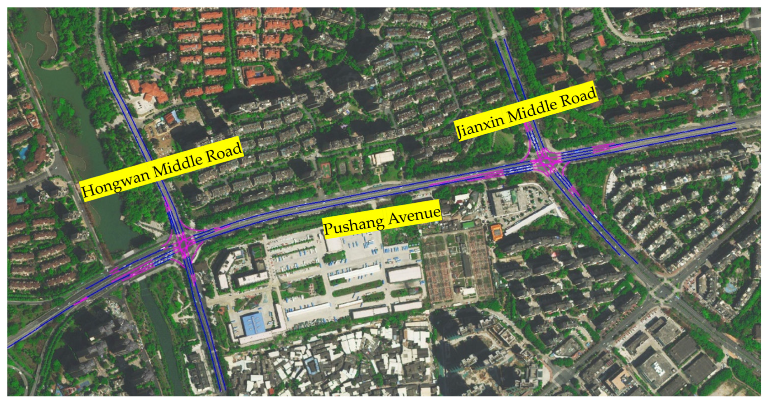
2.1. Architecture of Intersections

In the traffic management process at adjacent intersections with different cycles, the offset between the two intersections exhibits orderly variations as the signal cycle progresses. Such variations lead to periodic fluctuations in traffic flow between the two intersections, severely affecting traffic flow. It also causes vehicle queue length and delay time to increase significantly, further aggravating traffic congestion. It is necessary to avoid the offset between the two intersections falling into mismatched ranges to achieve optimized coordinated control. At the same time, the number of queued vehicles and those arriving before the queue dissipates in the through lanes of the downstream intersection needs to be reduced to minimize the waste of coordinated green light time. This, in turn, can improve the efficiency of the through traffic in the transition section.

This study selected two adjacent intersections in Fuzhou, China, as the research subjects: Pushang Avenue and Hongwan Middle Road, as well as Pushang Avenue and Jianxin Middle Road (see Figure 1). The chosen survey date was 20 September 2023, and the survey times were during the morning peak from 7:30 to 8:30 and the evening peak from 17:30 to 18:30. During the survey period, there were no traffic accidents on the roads or in the surrounding areas.

The architecture of the adjacent intersections analyzed in this study is shown in Figure 2. The architecture involves two intelligent traffic signals that use advanced 5G communication and perception technologies to obtain real-time information on the traffic signal phase, traffic flow, and road environment for the two intersections. Using data fusion, analysis, processing and interaction, and information exchange between vehicle-to-vehicle and vehicle-to-road, active control and guidance can be achieved. The main process involved collecting and preprocessing traffic information using radar–camera-integrated devices, traffic signal controllers, and roadside RSUs. The data were then transmitted to a cloud platform for analysis and optimization. Strategies such as extending green light durations, dynamically adjusting phase offsets, and guiding vehicle speeds were used to generate signal control and speed guidance plans. The signal control plan was implemented by adjusting signal timing via an upper-level computer, and the speed guidance plan was communicated to on-board units (OBUs) or roadside displays through vehicle-to-vehicle (V2V) and vehicle-to-infrastructure (V2I) communication systems optimizing traffic coordination and improving operational efficiency.

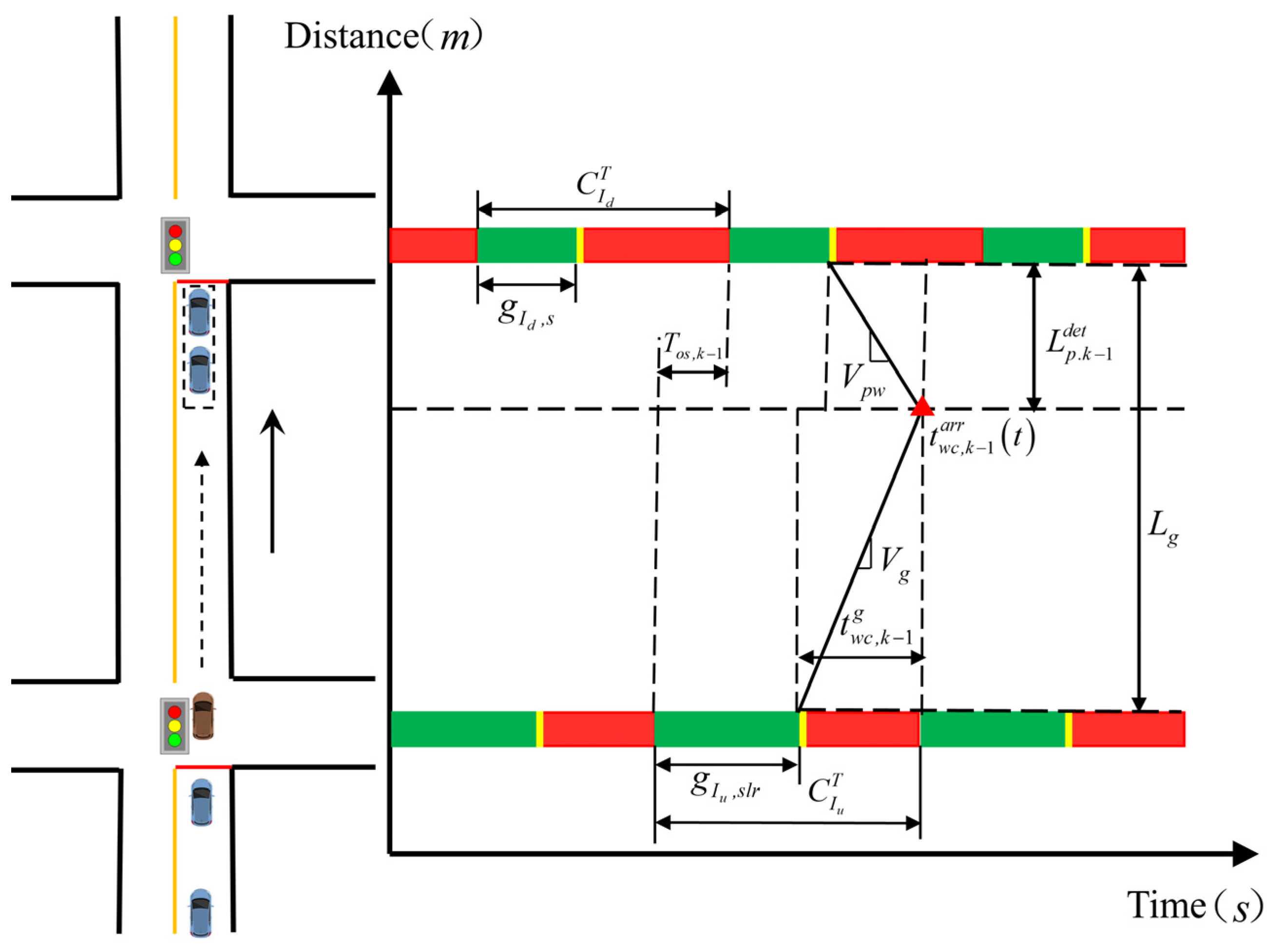
2.2. Periodic Offset Characteristics

Due to the different cycle lengths of the upstream and downstream intersections, the offset will shift in a fixed direction after each cycle, given the upstream intersection as a reference. The offset exhibits cyclical periodicity, meaning that after a certain number of upstream cycles, the offset will return to its initial state. With each repetition of the control cycle, the offset will sequentially shift, generating values for m steps. There are two possible transition cycles: a longer to shorter (L-S) cycle and a shorter to longer (S-L) cycle. For the L-S transition cycle, the generated offset, $T_{os,k}\left(k=1, 2, \cdots , \infty \right)$, can be derived as

$$\begin{array}{c}{T}_{os,k}=\left(k-⌊\frac{k}{m}⌋m\right)\Delta T\\ m=\left(\frac{C_{I_d}^T}{C_{I_u}^T-C_{I_d}^T}\right)\end{array}$$

(1)

where $k$ = cycle number at the upstream intersection, $⌊\frac{k}{m}⌋$ = lower integer of $\frac{k}{m}$, $m$ = number of (short) cycles at the upstream intersection for which the starts of the cycles coincide, $\Delta T$ = offset for an L-S cycle transition, and $C_{I_u}^T$,$C_{I_d}^T$ = cycle lengths at the upstream and downstream intersections, respectively.

For the S-L transition cycle, the generated offset, $T_{os,k}^{\prime }\left(k=1, 2, \cdots , \infty \right)$, can be derived as

$$\begin{array}{c}{T}_{os,k}^{\prime }=\left(k-⌊\frac{k}{m^{\prime }}⌋m^{\prime }\right)\Delta T\\ m^{\prime }=1+\left(\frac{C_{I_u}^T}{C_{I_d}^T-C_{I_u}^T}\right)\end{array}$$

(2)

where $⌊\frac{k}{m^{\prime }}⌋$ = lower integer of $\frac{k}{m^{\prime }}$, $m^{\prime }$ = number (long) cycles at the upstream intersection for which the starts of the cycles coincide, and $\Delta T^{\prime }$ = offset for an S-L cycle transition. To illustrate, given $C_{I_u}^T$ = 30 s and $C_{I_d}^T$ = 40 s, $m^{\prime }$ = 4, and $\Delta T^{\prime }$ = 10 s. Then, $T_{os,1}^{\prime }$ = 10 s, $T_{os,2}^{\prime }$ = 20 s, $T_{os,3}^{\prime }$ = 30 s, and $T_{os,4}^{\prime }$= 0 s. After this cycle, the previous sequence is repeated, starting with $T_{os,5}^{\prime }$ = 10 s.

In Equations (1) and (2), there is a transition from $T_{os,k-1}\to T_{os,k}\left(T_{os,k-1}^{\prime }\to T_{os,k}^{\prime }\right)$, where the offset increases or decreases by the duration of the cycle at the downstream intersection.

2.3. Queue-Length Models

Based on the periodic offset characteristics, three queue-length models are presented: (1) model for the queue length of vehicles that are delayed from the previous cycle, (2) model for the queue length of the vehicles arriving ahead of the schedule in the current cycle, and (3) model for the maximum queue length in the current cycle.

2.3.1. Model 1: Queue Length of Vehicles Delayed from Previous Cycle

From the moment when vehicles from all directions at the upstream intersection merge into the through phase, exiting at the downstream intersection after the green ends, the vehicle queuing begins. The length of the queue is determined by the number of vehicles that have not yet exited and can be determined by the arrival time of the last vehicle at the end of the queue. The specific details are shown in Figure 3.

The queue of vehicles from the previous cycle begins to form at the downstream intersection when the green from the previous cycle ends. This queue continues until the last vehicle arrives at the end of the queue. During this process, arriving vehicles create a queue wave with a propagation speed of V_pw. The expression for the queue length of vehicles delayed from the previous cycle is represented as $L_{p,k-1}^{\mathit{det}}$, which is given by

$$L_{p,k-1}^{\mathit{det}}=\frac{\left[L_g+\left(g_{I_u,slr}-g_{I_d,s}-T_{os,k-1}\right)\times V_g\right]\times V_{pw}}{V_g+V_{pw}}$$

(3)

where $L_g$ = distance between the stop line at the upstream intersection’s entrance lane and the stop line at the downstream intersection’s entrance lane, $V_g$ = speed at which vehicles can travel continuously without stopping, $g_{I_d,s}$ = duration of the green phase for the through movement at the downstream intersection, $g_{I_u,slr}$ = durations of the green phases for the through, left-turn, and right-turn movements at the upstream intersection, and $T_{os,k-1}$ = remaining offset value for cycle k − 1.

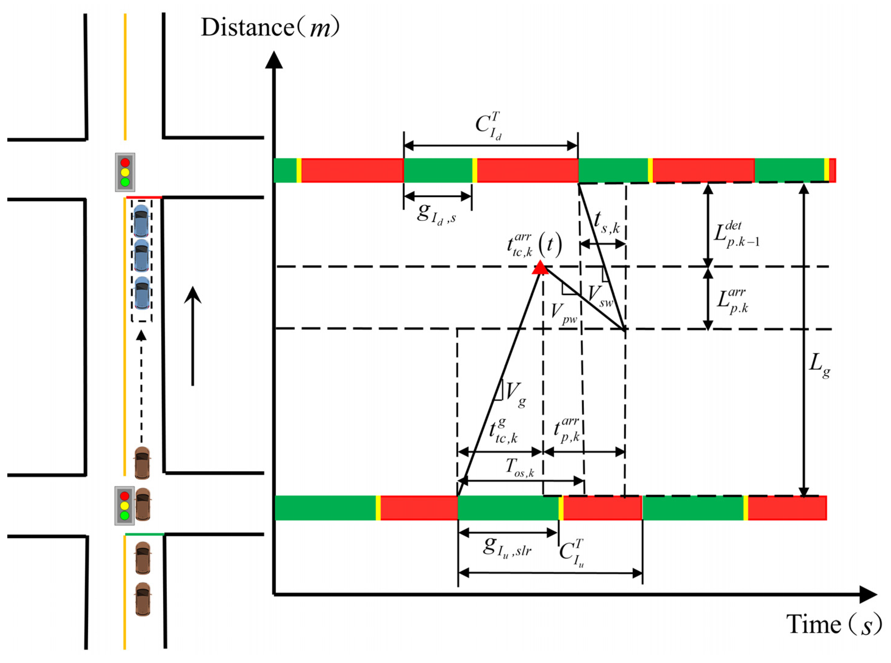
2.3.2. Model 2: Queue Length of Vehicles Arriving Ahead of Schedule in Current Cycle

Upon the activation of the green phase for the merging direction at the upstream intersection in the current operational cycle, if the vehicles merging from this direction arrive before the green phase for the through movement at the downstream intersection starts, they must come to a stop and wait behind the queue of vehicles delayed from the previous cycle. This action creates a new queue of vehicles, and the queuing time for subsequently joining vehicles is determined by the time of arrival of the first vehicle at the end of the queue and the moment when the queuing wave and stopping wave intersect, as shown in Figure 4.

When the leading vehicle merges from the upstream intersection during the current cycle’s green phase duration and reaches the end of the queue of delayed vehicles at the downstream intersection, the relationship equation for the initiation of queuing can be expressed as: $t_{tc,k}^{arr}\left(t\right)=t_{tc,k}^g+g_{I_u,k,slr}^b\left(t\right)$. In the current cycle, when the leading vehicle from the merging traffic reaches the end of the queue of delayed vehicles and comes to a stop, it generates a stopping wave propagating backward at a speed of $V_{pw}$. This causes subsequent arriving vehicles to closely follow the preceding queue, coming to a stop and waiting. After the green for the through movement at the downstream intersection is activated, the queued vehicles in front of the stop line will start to move one by one, creating a start-up wave propagating backward at a speed $V_{sw}$ toward the end of the queue. The maximum queue length at the intersection is reached when the start-up wave propagating backward meets the stopping wave generated by the arriving vehicles. Simultaneously, one can establish the relationship between the queue length of the arriving vehicles in the current cycle and offset $T_{os,k}$, as follows

$$T_{os,k}+\frac{L_{p,k-1}^{\mathit{det}}+L_{p,k}^{arr}}{V_{sw}}=\frac{L_g-L_{p,k-1}^{\mathit{det}}}{V_g}+\frac{L_{p,k}^{arr}}{V_{pw}}$$

(4)

Finally, the queue length of the arriving vehicles in the current cycle $L_{p,k}^{arr}$ is obtained as

$$L_{p,k}^{arr}=\frac{V_{pw}\times V_{sw}}{V_{pw}-V_{sw}}\times \left(\frac{L_g-L_{p,k-1}^{\mathit{det}}}{V_g}-\frac{L_{p,k-1}^{\mathit{det}}}{V_{sw}}-T_{os,k}\right)$$

(5)

To summarize, for an L-S (S-L) cycle transition, as the offset decreases (increases), the queue length of the delayed vehicles from the previous cycle gradually increases (decreases). There is a varying amount of change such that:

$$\Delta \left(\frac{L_{p,k-1}^{\mathit{det}}}{V_{sw}}-\frac{L_{p,k-2}^{\mathit{det}}}{V_{sw}}\right)>\Delta \left(\left|T_{os,k}-T_{os,k-1}\right|\right) (L-S\; cycle\; transition)$$

(6)

$$\Delta \left(\left|\frac{L_{p,k-1}^{\mathit{det}}}{V_{sw}}-\frac{L_{p,k-2}^{\mathit{det}}}{V_{sw}}\right|\right)>\Delta \left(T_{os,k}-T_{os,k-1}\right) (S-L\; cycle\; transition)$$

(7)

The change in the L-S (S-L) cycle transition results in the queue length of vehicles arriving ahead of the schedule in the current cycle gradually decreasing (increasing) over several consecutive cycles.

2.3.3. Model 3: Maximum Queue Length in Current Cycle

By combining the model for the queue length of delayed vehicles from the previous cycle and the model for the queue length of vehicles arriving ahead of schedule in the current cycle, one can jointly derive the model for the maximum queue length in the current cycle as

$$\begin{array}{cc}\hfill L_{p,k}^{\mathit{max}}& =L_{p,k-1}^{\mathit{det}}\times {\delta }^{\mathit{det}}+L_{p,k}^{arr}\times {\delta }^{arr}\hfill \\ & =\left\{\frac{\left[L_g+\left(g_{I_u,slr}-g_{I_d,s}-T_{os,k-1}\right) \times V_g\right] \times V_{pw}}{V_g + V_{pw}}\right\}\times {\delta }^{\mathit{det}}+\hfill \\ & \left\{\begin{array}{c}\frac{V_{pw} \times V_{sw}}{V_{pw}-V_{sw}}\times \\ \left\{\begin{array}{l}\frac{L_g-\frac{\left[L_g + \left(g_{I_u,slr} - g_{I_d,s} - T_{os,k-1}\right) \times V_g\right] \times V_{pw}}{V_g + V_{pw}}}{V_g}-\\ \frac{\frac{\left[L_g + \left(g_{I_u,slr} - g_{I_d,s} - T_{os,k-1}\right) \times V_g\right] \times V_{pw}}{V_g + V_{pw}}}{V_{sw}}-T_{os,k}\end{array}\right\}\end{array}\right\}\times {\delta }^{arr}\hfill \end{array}$$

(8)

where $L_{p,k}^{\mathit{max}}$ = maximum queue length in the current cycle, ${\delta }^{\mathit{det}}$ = categorical variable that can take on one of two possible values (0 and 1), indicating, respectively, the absence and presence of queued or delayed vehicles from the previous cycle, and ${\delta }^{arr}$ = categorical variable that can take on one of two possible values (0 and 1), indicating, respectively, the absence and presence of queued vehicles arriving ahead of schedule in the current cycle.

2.4. Maximum Queue Length

The vehicle queue length, developed using the periodic offset characteristics, varies according to the offset variation. Due to the correlation between the difference in the upstream and downstream intersections’ cycle lengths and the offset, changes in the queue length will impact the overall model trend. Therefore, controlling the variables can help establish fixed values and investigate their relationship with a single variable. Hence, the following were assumed: a high traffic volume condition for merging traffic, a transition section length of 800 m, and a range of values for the difference in cycle lengths between the upstream and downstream intersections between 10 s and 40 s, with an adjustment increment of 10 s. According to Equation (6), vehicle speed, stopping wave speed, and starting wave speed can be determined by varying the volume of merging traffic for through, left-turn, and right-turn movements at the upstream intersection. These values can be calculated based on the Greenshields relationships. The outcomes of the two transition types are shown in Figure 5.

The changes in the difference in cycle lengths between upstream and downstream intersections for the two transition types will result in alterations in the periodicity of queue length variations and the range of numerical changes. For an L-S cycle transition, as the difference in cycle lengths increases, the numerical values of the queue length become more evenly distributed across various operational cycles. The peak value gradually decreases, indicating an overall declining trend. Conversely, for an S-L cycle transition, as the difference in cycle lengths increases, the numerical values of the queue length exhibit more pronounced variations across different operational cycles. The minimum value gradually increases, indicating an overall upward trend.

3. Proposed Coordinated Control Method

3.1. Assumptions and Control Strategies

The proposed method involves five assumptions to simplify the control strategies. First, all controlled vehicles are connected and strictly adhere to the vehicle speed guidance strategy. Second, when vehicles enter the transition section’s speed guidance zone, they will only pass through based on the green phase time of the downstream intersection in the current or the next cycle. The scenario of speed guidance extending beyond two cycles and vehicles stopping and queuing for a second time is not considered. Third, the flow of vehicles merging from the non-coordinated right-turn phase is signal-controlled, and the phases for all three merging directions should be continuous and consecutive. Fourth, considering the speed limits of urban roads and primary highways in China, which range from 30 to 70 km per hour, and the fact that vehicles on certain roads can reach speeds of 70 km/h, the speed limit for this model was set at 70 km per hour to better explore the model’s control effects. However, due to safety considerations, speeds exceeding 60 km per hour should be used with caution. Finally, to ensure that the simulation objects can meet the proposed coordinated control optimization method, the phase sequences need to be re-optimized based on the original number of phases. The optimized phase sequences are shown in Figure 6.

To address this problem, the coordination involves three strategies: (1) green phase extension strategy at the downstream intersection, (2) dynamic adjustment of phase-difference strategy at the upstream and downstream intersections, and (3) queue-speed guidance strategy at the transition section. Strategy 1 timely extends the green phase time for the coordinated direction at the downstream intersection as it approaches its end to address the issue of queued vehicles. This strategy aims to reduce unnecessary delays for the queued vehicles. Simultaneously, Strategy 3 guides target vehicles to accelerate or decelerate as appropriate, based on the coordinated phase signal state and traffic flow conditions, to minimize the instances of vehicles coming to a stop and waiting.

3.2. Strategy 1: Green Phase Extension Strategy

For the assumed intersection signal phases, consider the coordinated phase direction at the downstream intersection, which is the westbound through. The non-coordinated phases that do not overlap with their green phases are split into the following: the first turn (eastbound left-turn), the fifth turn (northbound through right), and the sixth turn (southbound through left). The control objective is to extend the green phase time for the westbound through-coordinated direction when a vehicle is detected to be arriving within the unit green extension time. This extension aims to increase the green bandwidth in that direction while simultaneously reducing the green phase time for the non-coordinated directions to balance the phase cycle duration.

(a)

Determine the total amount of green phase time that can be reduced for each non-coordinated phase within the cycle while ensuring that the green phase time for each non-coordinated phase $g_{I_d,k,unco}^i$ is not less than its minimum green time $g_{I_d,k,unco}^{i,\mathit{min}}$ and the extended green phase time for the coordinated phase does not exceed the sum of the minimum green times $g_{I_d,k,co}^{\mathit{min}}$ for the non-coordinated phases plus the total available green phase time. That is,

$$g_{I_d,k,co}^{\mathit{max}}\le g_{I_d,k,co}^{\mathit{min}}+{\displaystyle \sum _{i=1,5,6}\left(g_{I_d,k,unco}^i-g_{I_d,k,unco}^{i,\mathit{min}}\right)}$$

(9)

(b)

Determine the extension time for a unit of green phase $\Delta g_{unit}^{le}$ when the green phase time for the westbound through-coordinated phase at the downstream intersection reaches the initially pre-set green phase time, based on the detectors of the vehicle arrivals within the unit green extension time $\Delta g_{unit}^{le}$, determining the extension amount $g_{I_d,k,co}^{le}$ for the green phase time of the coordinated phase in cycle k. This value should not exceed the sum of the green phase time, which can be reduced. The green phase time for the coordinated phase after extension, $g_{I_d,k,co}^{new}$, is given by

$$g_{I_d,k,co}^{new}=g_{I_d,k,co}^{\mathit{min}}+g_{I_d,k,co}^{le}$$

(10)

(c)

Sequentially reduce the green phase time $g_{I_d,k,unco}^i$ for each non-coordinated phase by the time increments defined by $\mathsf{\Delta }g=1 \mathrm{s}$ until the total reduction ${\displaystyle \sum \Delta g}$ matches the extension amount for the green phase time of the coordinated phase $g_{I_d,k,co}^{le}$. Meanwhile, the following constraints ensure that the remaining green phase time $g_{I_d,k,unco}^{i,re}$ for each non-coordinated phase does not fall below the minimum green time $g_{I_d,k,unco}^{i,\mathit{min}}$ to balance the phase cycle duration:

$$\left\{\begin{array}{c}{g}_{I_d,k,unco}^{i,re}=g_{I_d,k,unco}^i-\Delta g\\ s.t.{\displaystyle \sum \Delta g=}{g}_{I_d,k,co}^{le}\\ g_{I_d,k,unco}^{i,re}\ge g_{I_d,k,unco}^{i,min}\end{array}\right.i=1,5,6$$

(11)

After adjusting and allocating the phases at the downstream intersection, the phase cycle duration $C_{I_d,k}^{T,new}$ is updated and balanced by

$$C_{I_d,k}^{T,new}=g_{I_d,k,co}^{new}+{\displaystyle \sum _{i=1,5,6}{g}_{I_d,k,unco}^{i,re}}$$

(12)

3.3. Strategy 2: Dynamic Offset Adjustment Strategy

This strategy is based on the premise that there is a compatible phase sequence at the upstream intersection, meaning that the phase sequence for the upstream intersection’s through, left-turn, and right-turn traffic merging directions should be continuous and consecutive.

3.3.1. Determining Offset Adjustment

First, based on the signal phase status of the downstream intersection’s coordinated phase (westbound through) at the end of each cycle of the upstream intersection, estimate the number of queued vehicles for westbound through traffic in the transition section for the current cycle among the merging traffic streams of westbound through, northbound left turn, and southbound right turn. Second, considering the arrival of traffic from the upstream intersection in the next cycle for the westbound through merging direction, determine the adjustment offset for the next operational cycle of both intersections. Finally, calculate the difference between the offsets before and after adjustment to obtain the adjustment amount. The steps of this adjustment are mathematically presented in Appendix A.

3.3.2. Determining Number of Phases Available for Adjustment

Based on the phase situation of the downstream intersection at the end of the phase cycle of the upstream intersection, determine the number of non-coordinated phases at the downstream intersection that can be adjusted in the subsequent cycle duration by

$$Phase=\left\{\begin{array}{c}3,g_{I_d,k,1}^b\left(t\right)\le C_{I_u,k}^e\left(t\right)<g_{I_d,k,3}^e\left(t\right)\\ 2,g_{I_d,k,3}^e\left(t\right)\le C_{I_u,k}^e\left(t\right)<g_{I_d,k,4}^e\left(t\right)\\ 1,g_{I_d,k,4}^e\left(t\right)\le C_{I_u,k}^e\left(t\right)<g_{I_d,k,5}^e\left(t\right)\end{array}\right.$$

(13)

where $Phase$ = number of phases that can be adjusted, $g_{I_d,k,n}^b\left(t\right)$ = green start time for phase n at the downstream intersection in k, $g_{I_d,k,n}^e\left(t\right)$ = green end time for phase n at the downstream intersection in k, and $C_{I_u,k}^e\left(t\right)$ = signal phase end time for the upstream intersection in cycle k.

3.3.3. Determine Maximum Green Time Available for Adjustment

By assessing the relationship between the end time of the signal phase at the upstream intersection at the end of its cycle and the minimum green time required for that phase at the downstream intersection, determine the maximum green time available for adjustment for each non-coordinated phase as

$$g_{I_d,k,n}^{ad,\mathit{max}}=\left\{\begin{array}{l}{g}_{I_d,k,n}^e\left(t\right)-g_{I_d,k,n}^{\mathit{min}}\left(t\right),g_{I_d,k,n-1}^e\left(t\right)<C_{I_u,k}^e\left(t\right)\le g_{I_d,k,n}^{\mathit{min}}\left(t\right)\hfill \\ g_{I_d,k,n}^e\left(t\right)-C_{I_u,k}^e\left(t\right),g_{I_d,k,n}^{\mathit{min}}\left(t\right)<C_{I_u,k}^e\left(t\right)\le g_{I_d,k,n}^e\left(t\right)\hfill \end{array}\right.$$

(14)

where $g_{I_d,k,n}^{ad,\mathit{max}}$ = maximum green time available for adjustment for the n phase in cycle k at the downstream intersection and $g_{I_d,k,n}^{\mathit{min}}\left(t\right)$ = ending time of the minimum green time required for the n phase in cycle k at the downstream intersection. In addition, calculate the maximum green time available for adjustment in the current cycle at the downstream intersection as

$$g_{I_d,k}^{ad,\mathit{max}}=\left\{\begin{array}{l}{g}_{I_d,k,3}^{ad,\mathit{max}}+\left(g_{I_d,k,4}^e\left(t\right)-g_{I_d,k,4}^{\mathit{min}}\left(t\right)\right)+\left(g_{I_d,k,5}^e\left(t\right)-g_{I_d,k,5}^{\mathit{min}}\left(t\right)\right),Phase=3\hfill \\ g_{I_d,k,4}^{ad,\mathit{max}}+\left(g_{I_d,k,5}^e\left(t\right)-g_{I_d,k,5}^{\mathit{min}}\left(t\right)\right)\hspace{1em}\hspace{1em}\hspace{1em}\hspace{1em}\hspace{1em}\hspace{1em}\hspace{1em}\hspace{1em}\hspace{1em},Phase=2\hfill \\ g_{I_d,k,5}^{ad,\mathit{max}}\hspace{1em}\hspace{1em}\hspace{1em}\hspace{1em}\hspace{1em}\hspace{1em}\hspace{1em}\hspace{1em}\hspace{1em}\hspace{1em}\hspace{1em}\hspace{1em}\hspace{1em}\hspace{1em}\hspace{1em}\hspace{1em}\hspace{1em}\hspace{1em},Phase=1\hfill \end{array}\right.$$

(15)

where $g_{I_d,k}^{ad,\mathit{max}}$ = maximum green time available for adjustment at the downstream intersection in cycle $k$.

3.3.4. Updating Phase Signal Timing

Step 1: The adjustment amount of the offset $\Delta T_{k+1,os}$ is allocated in sequence according to the number of phases that can be adjusted at the downstream intersection. If an increase in the offset is required in cycle k+1, then in cycle k, 1 s of green time is added sequentially to each of the non-coordinated phases that can be adjusted. If $\Delta T_{k+1,os}=0$, it indicates that the allocation has been completed. If a reduction in offset is required in cycle k+1, then in cycle k, 1 s of green time is reduced sequentially for each non-coordinated phase that is available for adjustment. If $\Delta T_{k+1,os}=0$ or $\Delta T_{k+1,os,n}^{ad}=g_{I_d,k}^{ad,\mathit{max}}$, the maximum available green signal time for adjustment has been reached, it indicates that the allocation is complete.

Step 2: After adjusting the green signal times for each phase, update the cycle duration and offset for that cycle by

$$\left\{\begin{array}{l}{C}_{I_d,k}^{T,ad}={\displaystyle \sum _n{g}_{I_d,k,n}^{ad}}+n\times A\\ T_{os,k+1}=g_{I_d,k,s}^b\left(t\right)+C_{I_{d,}k}^{T,ad}-g_{I_u,k+1,s}^b\left(t\right)\end{array}\right.$$

(16)

where $C_{I_d,k}^{T,ad}$ = updated green signal times for the phases at the downstream intersection in cycle k, $g_{I_d,k,n}^{ad}$ = adjusted green signal time for phase n at the downstream intersection in cycle k, A is yellow signal time (3 s), $T_{os,k+1}$ = offset for cycle k + 1, $g_{I_d,k,s}^b\left(t\right)$ is the moment when the green for the through phase with cycle k + 1, at the downstream intersection is activated, and $g_{I_u,k+1,s}^b\left(t\right)$ = initiation moment of the green for the through phase with cycle k + 1 at the upstream intersection.

3.4. Strategy 3: Queue-Speed Guidance Strategy for Transition Section

The speed guidance for the queue is based on various arrival scenarios that vehicles may encounter when traveling at normal speeds under different signal phases. Without considering secondary stopping and queuing, relevant control strategies are formulated.

①

If the downstream intersection’s coordinated phase is in the green signal state when the target queue approaches the guidance area, with sufficient remaining green time, or if it is in the red signal state with a relatively short remaining red time, and there are no vehicles ahead or any traffic that could affect the movement of the target queue, then the queue can be guided to travel at the maximum speed $V_{\mathit{max}}$ allowed by the road. Refer to Equation (17) for guidance speed $V_{ta,fle}^l$ and Figure 7a for the illustrative scenario.

$$V_{ta,fle}^l=V_{\mathit{max}}$$

(17)

②

If the downstream intersection’s coordinated phase is in the green signal state with sufficient remaining green time when the target queue reaches the guidance area, and there is a stable-moving queue ahead, the target queue should be guided to catch up with the trailing vehicle of the preceding queue to form a platoon of vehicles. The target queue should closely follow the preceding queue to cross the intersection stop line. Refer to Equation (18) for guidance speed $V_{ta,fle}^l$ and Figure 7b for the illustrative scenario.

$$V_{ta,fle}^l=\frac{L_{ta,fle}^{hc}\left(t\right)}{L_{ah,fle}^{tc}\left(t\right)\times 3.6/V_{ah,fle}}$$

(18)

where $L_{ta,fle}^{hc}\left(t\right)$ = distance from the front vehicle of the target queue to the intersection stop line at the moment of arrival in the guidance area, $L_{ah,fle}^{tc}\left(t\right)$ = distance from the rear vehicle of the preceding queue to the intersection stop line at the moment when the target queue is being guided, and $V_{ah,fle}$ = speed at which the preceding queue is traveling.

③

If the downstream intersection’s coordinated phase is in the green signal state when the target queue arrives at the guidance area, and the queued vehicles ahead have not yet dispersed, or if it is in the red signal state with a significant remaining red time, to avoid the target queue from coming to a stop and waiting, the front vehicle of the target queue should be guided to drive to the rear of the queued vehicles in front. When the queue-starting wave reaches the last vehicle in the queue, the target queue can then closely follow the queued vehicles to cross the intersection stop line. Refer to Equation (19) for guidance speed $V_{ta,fle}^l$ and Figure 7c for the illustrative scenario.

$$V_{ta,fle}^l=\frac{L_{ta,fle}^{hc}\left(t\right)-L_{I_d,k,s}^q}{g_{I_d,k,s}^b\left(t\right)-t\left(n\right)+L_{I_d,k,s}^q/V_{sw}}$$

(19)

where $L_{I_d,k,s}^q$ = queue length of the queued vehicles in the downstream intersection’s coordinated through direction with cycle k and $t\left(n\right)$ = current moment, which is the time when the front vehicle of the target queue arrives at the guidance area.

Figure 7. Control scenario of speed guidance.

Figure 7. Control scenario of speed guidance.

4. Simulation Experiments

4.1. Experimental Design

To evaluate the effectiveness of the proposed method, a custom control program was developed using Visual Studio 2020 and VISSIM 4.3 simulation software. This allowed the creation of a customized simulation platform for vehicle–road collaboration. Various orthogonal adaptive experiments were designed, considering multiple factors, to investigate the control optimization effects. The primary objective of the experimental design is to investigate the adaptability of the optimization method under variations in four influencing factors: inflow traffic volume, transition segment length, desired speed, and the difference in cycle lengths between upstream and downstream intersections. The ranges and adjustment step sizes of the influencing factors of the adaptive experiments are shown in

Table 1. Ranges and adjustment step sizes of the influencing factors.

Influencing Factor	Range	Adjustment Step Size
Inflow traffic volume (pcu/h)	[1000, 3000]	500
Transition segment length (m)	[440, 1240]	200
Desired speed (km/h)	[30, 70]	10
Difference in cycle lengths (s) a	[10, 50]	10

^a Difference in cycle lengths of the upstream and downstream intersections.

.

The relevant simulation parameter inputs into the VISSIM software are shown in

Table 2. VISSIM traffic simulation parameter setting.

Simulation Name	Value
Simulation duration (s)	3600
Maximum acceleration (m/s2)	2.5
Minimum acceleration (m/s2)	−2.5
Response time (s)	1.5
Vehicle type	Car, HGV a, Bus
Percentage of vehicles	0.7, 0.1, 0.2
Lane width (m)	3.5
simulation.RandomSeed	40

^a Heavy goods vehicle.

. After simulation processing, evaluation indicators such as straight-through capacity, average queue length, average vehicle delay, average travel time per vehicle, and average number of stops per vehicle were obtained for subsequent result analysis. Next, the combination of influencing factors with the best optimization effects in the adaptive experiments was selected as the experimental group. For comparison, two control groups were designed: Control Group 1, where the two intersections were optimized separately without applying the control strategy proposed in this paper, and Control Group 2, where the two intersections used the same cycle and employed the unidirectional coordination control method on the main road.

The adaptive experiments utilize SPSS 27 data analysis software to design a four-factor, five-level orthogonal experiment. A random number of seed of 300 was set, generating a total of 25 sets of experimental combinations for each of the two transition types, resulting in a total of 50 sets of experimental combinations. Additionally, 25 control groups will be established for each of the two transition types with the same factor values but without the application of the coordinated control optimization method.

4.2. Analysis and Results

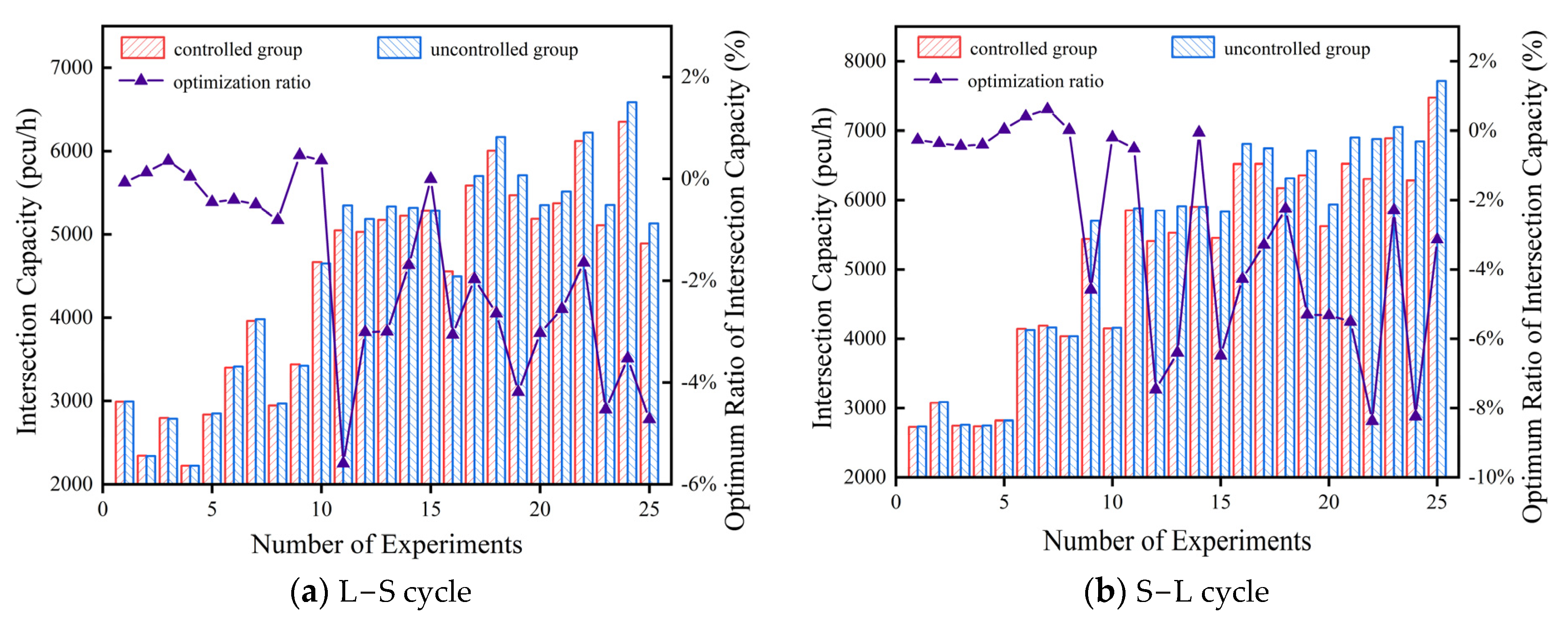
4.2.1. Analysis of Downstream Intersection Performance Intersection Capacity

The comparison of control effects on the downstream intersection for the two transition types under low-inflow traffic conditions is shown in Figure 8. The optimal capacity ratio of the downstream intersection fluctuates around 0%, indicating that the application of the control strategies has a relatively mild impact on capacity under these conditions. As the inflow traffic flow increases, the optimal ratio remains negative, indicating that applying the control strategies under these conditions leads to some decrease in the capacity of the downstream intersection but within an acceptable range.

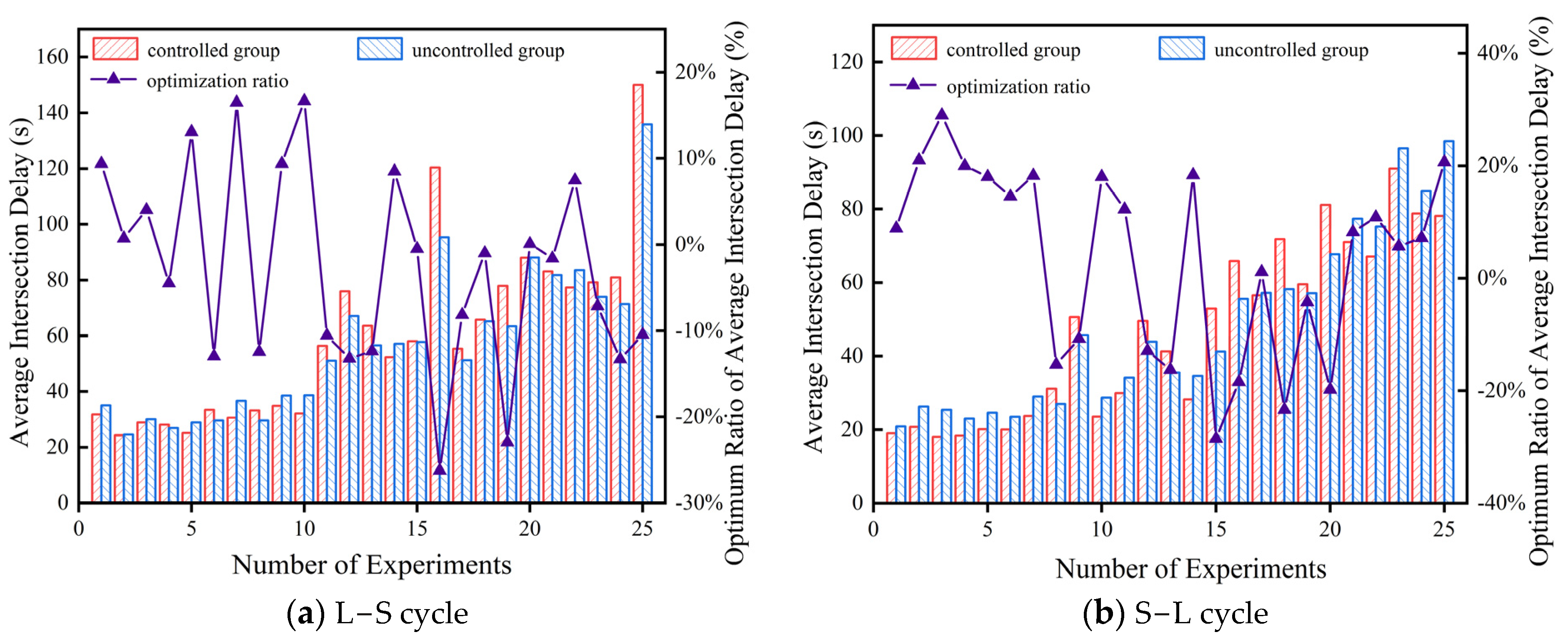
Intersection Average Vehicle Delay

The optimum ratio of the intersection average vehicle delay time of the downstream intersection exhibits significant fluctuations for the two transition types, as shown in Figure 9. Combinations of strategies were observed that yielded better results and others that yielded worse results. This indicates that under the combined influence of the four relevant factors, applying coordinated control strategies to the downstream intersection may have either a positive or negative impact on the average vehicle delay time.

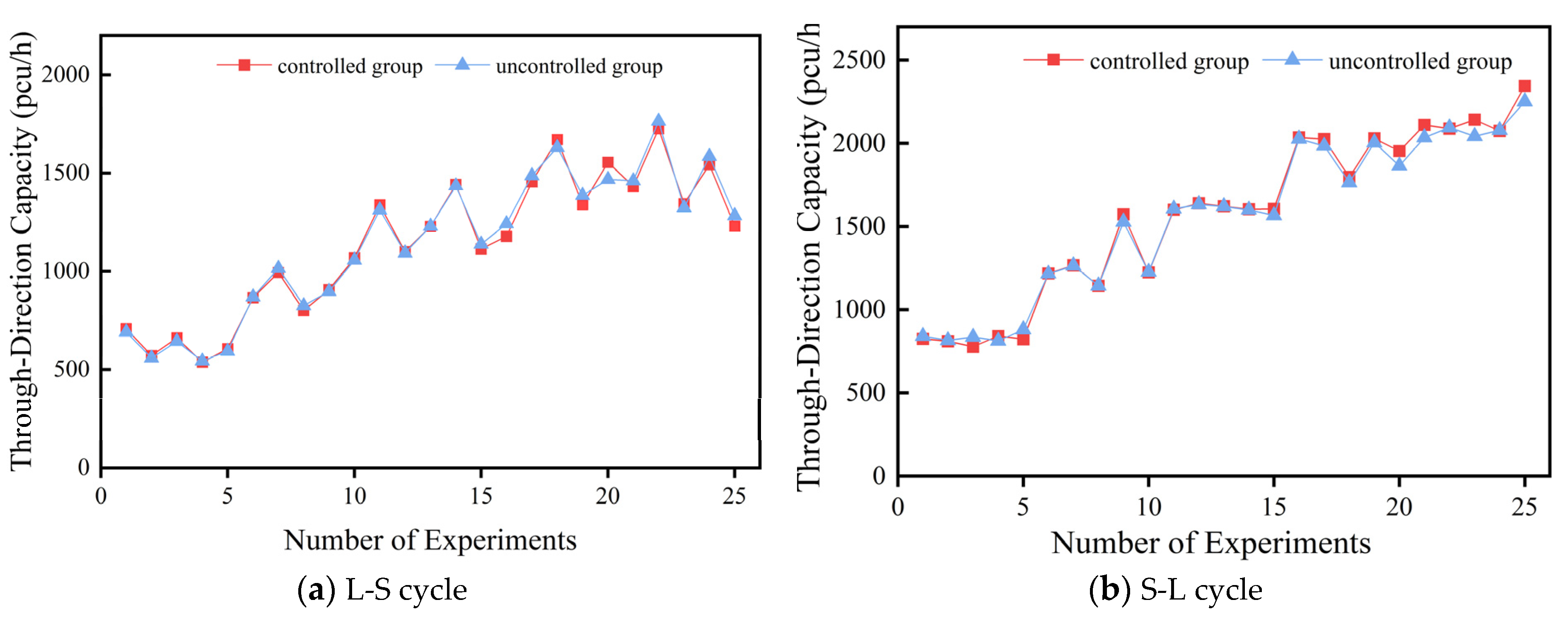
4.2.2. Analysis of Coordinated Through-Direction Performance Capacity

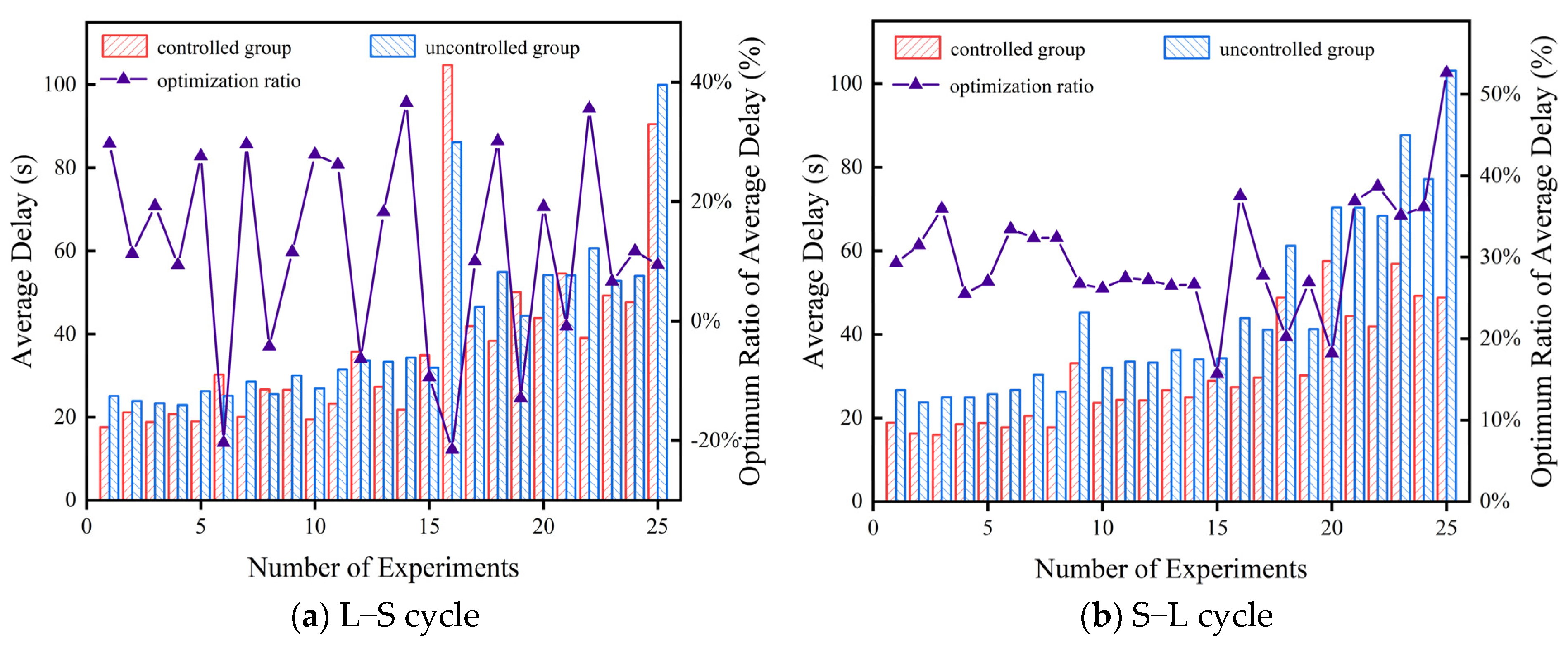
The analysis focuses on the numerical values and changes in the coordinated through-direction traffic capacity of the controlled group relative to the uncontrolled group, as shown in Figure 10. It can be observed that the numerical values of the through-traffic capacity in the experimental group and the control group are similar, and their fluctuation patterns are consistent. SPSS was used to perform the Mann–Whitney U test, and the results indicate $P=0.938>\alpha =0.05$. The analysis reveals that there is no significant difference between the two groups of experimental data, demonstrating that the multi-strategy combined optimization method has no significant impact on the traffic capacity of the coordinated through direction.

Average Delay

After applying coordinated control strategies to both transition types, the average vehicle delay time significantly decreases for most combinations of influencing factors, indicating a noticeable optimization effect, as shown in Figure 11.

For an L-S cycle transition, the optimization ratio of average vehicle delay time in the controlled group relative to the uncontrolled group fluctuates significantly, ranging from 0 to −40% overall. In particular, in the scheme combinations number 14, 18, and 22, the optimization effects are relatively good. However, in the scheme combinations number 6, 8, 12, 15, 16, and 19, the optimization effects are relatively poor, and the reduction ratio is negative. An analysis reveals that the scheme combinations with better optimization effects have a cycle length difference of 10 s, while the ones with poorer optimization effects have larger cycle length differences, such as 40 s or 50 s. This is because when the difference in cycle lengths between upstream and downstream intersections is larger, the cycle length at the downstream intersection becomes shorter. This reduces the optimization space for dynamic phase adjustment and green extension for coordinated phases at the downstream intersection. As a result, the coordinated control strategy is less effective. Conversely, when the cycle length difference is smaller, the coordinated control effect becomes more significant.

For an S-L cycle transition, the optimization ratio of average vehicle delay time in the controlled group relative to the uncontrolled group tends to stabilize. Generally, it falls within the range of 15% to 55%. Compared to the L-S cycle transition, the optimization effect is more prominent in this case. In particular, the scheme combination numbers 21, 22, 23, 24, and 25 exhibit relatively good optimization effects, while numbers 15, 18, and 20 show relatively poor optimization effects. An analysis reveals that the scheme combinations with better optimization effects in the former case have an inflow traffic volume of 3000 pcu/h, indicating that the proposed coordinated control strategy is more effective in optimizing high-flow conditions in this transition type. In contrast, the scheme combinations with poorer optimization effects in the latter case have desired speeds ranging from 50 km/h to 55 km/h. The reason for this result is that when the desired speed is lower, it is not conducive to implementing the speed guidance strategy in the coordinated control optimization method. This leads to the inability of the through-arriving queue to catch up with the queued vehicles ahead promptly, resulting in the waste of phase green time and an increase in the number of through-arriving vehicles waiting.

4.2.3. Orthogonal Analysis Results

The results of the orthogonal analysis are presented in

Table 3. Analysis of the orthogonal experimental range for the coordinated through direction and the corresponding optimal ratio of average delay ^a.

Transition Type	Analysis Indicators	Influencing Factor
		Inflow Traffic Volume (pcu/h)	Transition Section Length (m)	Desired Speed (km/h)	Difference in Cycle Lengths (s)
L-S cycle	Best level	2000	1240	65	10
	Worst level	2500	440	60	40
S-L cycle	Best level	3000	440	70	50
	Worst level	1500	1040	50	30
L-S cycle	$R$	0.17	0.13	0.06	0.38
S-L cycle	$R$	0.36	0.11	0.22	0.14

^a Ratio of the average delay (s) of the coordinated through direction before and after optimizing the signal timing.

. The orthogonal analysis evaluates the optimum ratio of the average vehicle delay in the coordinated through direction as the target variable using the range method. The analysis considers the larger-is-better criterion for the best level and the smaller-is-better criterion for the worst level. This provides the range (extreme values), reflecting the importance of each factor in influencing the experimental results. It also yields the best and worst levels within the proposed range of factors.

Based on the results of Table 2, for the L-S cycle transition, the importance of each factor in influencing the experimental results, from most to least significant, is as follows: cycle length difference > inflow traffic volume > transition segment length > desired speed. The optimization effect of the proposed coordinated control method is at its best when the inflow traffic volume is 2000 pcu/h, the transition segment length is 1240 m, the desired speed is 65 km/h, and the cycle length difference is 10 s. Conversely, the optimization effect is at its worst when the inflow traffic volume is 2500 pcu/h, the transition segment length is 440 m, the desired speed is 60 km/h, and the cycle length difference is 40 s. These two combinations can be denoted as (2000, 1240, 65, 10) and (2500, 440, 60, 40). When the traffic volume is 3000 pcu/h, the transition segment length is 440 m, the desired speed is 70 km/h, and the cycle length difference is 50 s, the optimization effect of the proposed coordinated control method is at its best. Conversely, when the traffic volume is 1500 pcu/h, the transition segment length is 1040 m, the desired speed is 50 km/h, and the cycle length difference is 30 s, the optimization effect is at its worst. These two combinations can be denoted as (3000, 440, 70, 50) and (1500, 1040, 50, 30). However, in practical applications, considering safety factors, speeds exceeding 60 km per hour should be carefully considered in conjunction with the actual situation.

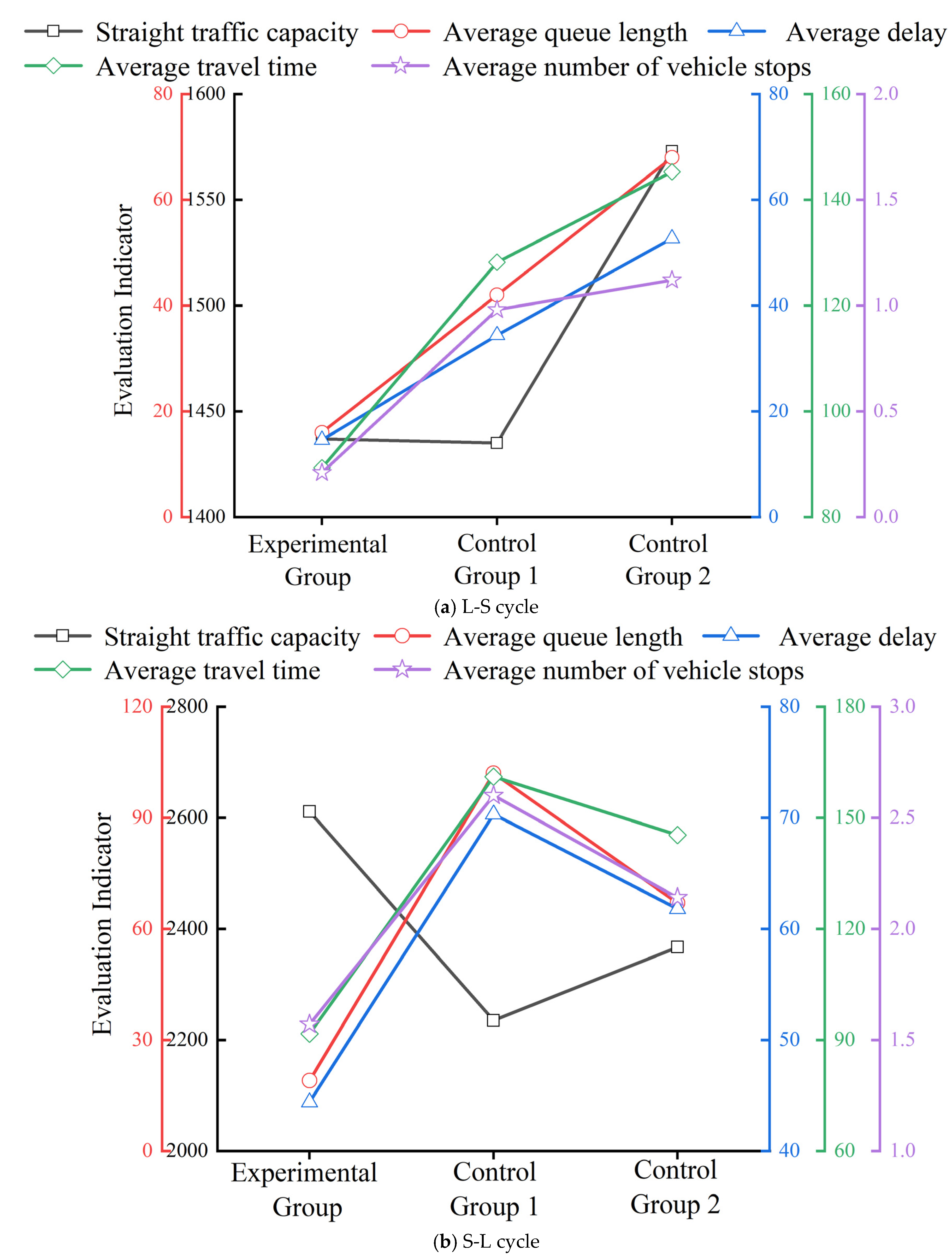
4.2.4. Comparative Results

In the comparative experiment of L-S cycle transition, for Control Group 1, the upstream and downstream cycle lengths were set to 180 s and 170 s, respectively. For Control Group 2, the cycle length was set to 180 s. The four influencing factors for all three groups were set to (2000, 1240, 65, 10). After conducting the simulation experiments, the output results for relevant evaluation indicators are shown in Figure 12a. It was found that, compared to Control Group 1, the experimental group had a 0.1% increase in straight-through capacity, a 61.9% decrease in average queue length, a 57.6% decrease in average vehicle delay time, a 30.3% decrease in average vehicle travel time, and a 78.6% decrease in average stops per vehicle. Compared to Control Group 2, the experimental group had an 8.6% decrease in straight-through capacity, a 76.5% decrease in average queue length, a 72.2% decrease in average vehicle delay time, a 38.5% decrease in average vehicle travel time, and an 81.3% decrease in average stops per vehicle.

In the comparative experiment of S-L cycle transition, for Control Group 1, the upstream and downstream cycle lengths were set to 160 s and 210 s, respectively. For Control Group 2, the cycle length was set to 210 s. The four influencing factors for all three groups were set to (3000, 440, 70, 50). After conducting the simulation experiments, the output results for relevant evaluation indicators are shown in Figure 12b. It was found that, compared to Control Group 1, the experimental group had a 16.8% increase in straight-through capacity, an 81.4% decrease in average queue length, a 36.8% decrease in average vehicle delay time, a 43.1% decrease in average vehicle travel time, and a 39.6% decrease in average stops per vehicle. Compared to Control Group 2, the experimental group had a 10.3% increase in straight-through capacity, a 71.6% decrease in average queue length, a 28.2% decrease in average vehicle delay time, a 36.9% decrease in average vehicle travel time, and a 26.6% decrease in average stops per vehicle.

In summary, the results indicate that the three proposed combinations of coordinated control strategies can significantly reduce the queue length in the through lanes while reducing the number of vehicles stops, thus improving the efficiency of traffic flow in the coordinated direction between adjacent intersections with different cycle lengths, all while maintaining the existing through-traffic capacity.

5. Conclusions

This paper has proposed a multi-strategy vehicle–road coordinated control method for unequal-cycle adjacent intersections. The strategy includes coordinated phase green extension for the downstream intersection, dynamic phase offset adjustment of the upstream intersection, and speed guidance for queued vehicles on the transition section. The proposed method can effectively reduce queuing and delay at the downstream intersection. Based on this study, the following comments are offered:

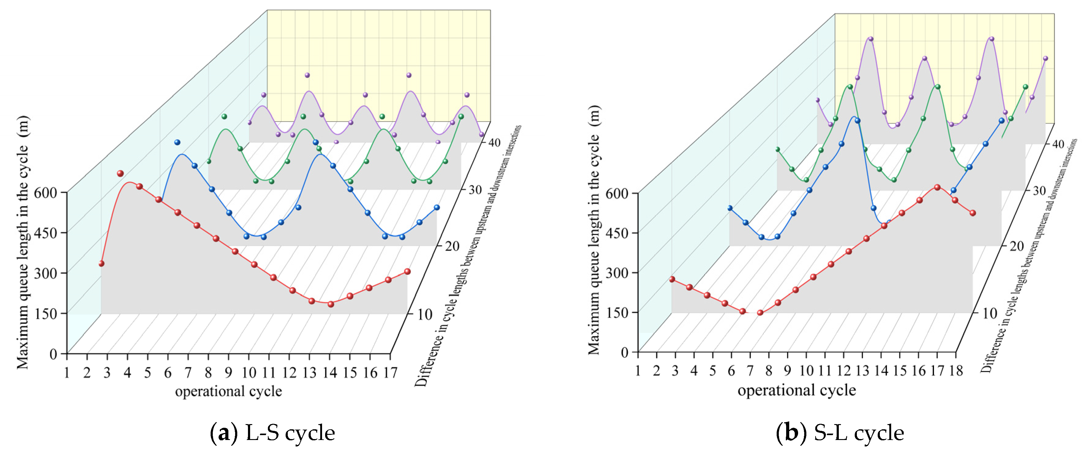
• The multi-strategy integrated method was validated using adaptive and comparative simulation experiments. The results showed that for an L-S cycle transition, the influencing factors are the following (ranked in decreasing order of importance): cycle length difference (10 s), inflow traffic volume (2000 pcu/h), transition segment length (1240 m), and desired speed (65 km/h), where the optimal values are shown in parentheses. For an S-L cycle transition, the influencing factors are inflow traffic volume (3000 pcu/h), desired speed (70 km/h), cycle length difference (50 s), and transition segment length (440 m).
• The proposed control strategies effectively reduce queue lengths, the number of stops, average vehicle delay time, and travel time for single-direction through lanes while improving the efficiency of the through traffic in the coordinated through direction between the adjacent intersections. This improvement is achieved while maintaining the original through traffic capacity.
• This study focuses on improving the passing efficiency for vehicles in one direction, and less attention was given to the coordinated control of the two-way traffic flow. It is hoped that the proposed methodology will be a valuable first step to optimizing the performance of two-way traffic flows at adjacent intersections with unequal cycles.
• The coordinated control method mentioned in this text requires pre-setting traffic signal control schemes, resulting in a lack of autonomy and flexibility in the optimization effect. Future research can incorporate optimization control algorithms within traffic signal controllers according to different optimization objectives, allowing intersections to automatically generate signal control schemes, thereby further enhancing the effectiveness of coordinated control.

References

1. Ni, J.; Chen, J.; Xie, W.; Shao, Y. The impacts of the traffic situation, road conditions, and driving environment on driver stress: A systematic review. Transp. Res. Part F Traffic Psychol. Behav. 2024, 103, 141–162. [Google Scholar] [CrossRef]
2. Fournier, N. Hybrid pedestrian and transit priority zoning policies in an urban street network: Evaluating network traffic flow impacts with analytical approximation. Transp. Res. Part A Policy Pract. 2021, 152, 254–274. [Google Scholar] [CrossRef]
3. Ren, F.; Dong, W.; Zhao, X.; Zhang, F.; Kong, Y.; Yang, Q. Two-layer coordinated reinforcement learning for traffic signal control in traffic network. Export Syst. Appl. 2024, 235, 121111. [Google Scholar] [CrossRef]
4. Gao, Y.; Qu, Z.; Song, X.; Yun, Z.; Zhu, F. Coordinated perimeter control of urban road network based on traffic carring capacity model. Simul. Model. Pract. Theory 2023, 123, 102680. [Google Scholar] [CrossRef]
5. Cao, J.; Hu, D.; Luo, Y.; Qiu, T.; Ma, Z. Exploring the impact of a coordinated variable speed limit control on congestion distribution in freeway. J. Traffic Transp. Eng. (Engl. Ed.) 2015, 2, 167–178. [Google Scholar] [CrossRef]
6. Morgan, J.T.; Little, J.D.C. Synchronizing traffic signals for maximal bandwindth. Oper. Res. 1964, 12, 807–1051. [Google Scholar] [CrossRef]
7. Gartner, N.H.; Assmann, S.F.; Lasaga, F.; Hous, D.L. Multiband—A Variable-Bandwidth Arterial Progression Scheme. Transp. Res. Rec. J. Transp. Res. Board 1990, 1287, 212–222. [Google Scholar]
8. Hu, H.; Liu, H.X. Arterial offset optimization using archived high-resolution traffic signal data. Transp. Res. Part C Emerg. Technol. 2013, 37, 131–144. [Google Scholar] [CrossRef]
9. Zhou, H.; Hawkins, H.G.; Zhang, Y. Arterial signal coordination with uneven double cycling. Transp. Res. Part A Policy Pract. 2017, 103, 409–429. [Google Scholar] [CrossRef]
10. Brilon, W.; Wu, N.; Koenig, R. Delays and Queue Lengths at Traffic Signals with Two Greens in One Cycle. Transp. Res. Rec. 2022, 2677, 828–838. [Google Scholar] [CrossRef]
11. Kesur, B. Optimization of Mixed Cycle Length Traffic Signals. J. Adv. Transp. 2024, 48, 431–442. [Google Scholar] [CrossRef]
12. Mukhtar, H.; Adil, A.; Alahmari, S.; Yonbawi, S. CCGN: Centralized collaborative graphical transformer multi-agent reinforcement learning for multi-intersection signal free-corridor. Neural Netw. 2023, 166, 396–409. [Google Scholar] [CrossRef]
13. Ducourthial, B.; Cherfaoui, V.; Fuhrmann, T.; Bonnet, S. Experimentation of a road hazard anticipation system based on vehicle cooperation. Veh. Commun. 2022, 36, 1000486. [Google Scholar] [CrossRef]
14. Shi, Y.; Han, Q.; Shen, W.; Wang, X. A Multi-Layer Collaboration Framework for Industrial Parks with 5G Vehicle-to-Everything Networks. Engineering 2021, 7, 818–831. [Google Scholar] [CrossRef]
15. Li, H.; Zhang, J.; Sun, X.; Niu, J.; Zhao, X. A survey of vehicle group behaviors simulation under a connected vehicle environment. Phys. A Stat. Mech. Its Appl. 2022, 603, 127816. [Google Scholar] [CrossRef]
16. Ma, X.; Ma, D.; Yuan, J.; Hao, S. Bandwidth optimisation and parameter analysis at two adjacent intersections based on set operations. IET Intell. Transp. Syst. 2019, 14, 684–692. [Google Scholar] [CrossRef]
17. Münder, M.; Carbon, C. Howl, whirr, and whistle: The perception of electric powertrain noise and its importance for perceived quality in electrified vehicles. Appl. Acoust. 2022, 185, 108412. [Google Scholar] [CrossRef]
18. Ayoub, J.; Yang, X.J.; Zhou, F. Modeling dispositional and initial learned trust in automated vehicles with predictability and explainability. Transp. Res. Part F Traffic Psychol. Behav. 2021, 77, 102–116. [Google Scholar] [CrossRef]
19. Deng, J.; Wu, X.; Wang, F.; Li, S.; Wang, H. Analysis and Classification of Vehicle-Road Collaboration Application Scenarios. Procedia Comput. Sci. 2022, 208, 111–117. [Google Scholar] [CrossRef]
20. Xing, Y.; Lv, C.; Cao, D.; Hang, P. Toward human-vehicle collaboration: Review and perspectives on human-centered collaborative automated driving. Transp. Res. Part C Emerg. Technol. 2021, 128, 103199. [Google Scholar] [CrossRef]
21. Wu, W.; Li, P.; Zhang, Y. Modelling and simulation of vehicle speed guidance in connected vehicle environment. Int. J. Simul. Model. 2015, 14, 145–147. [Google Scholar] [CrossRef]
22. Tiaprasert, K.; Zhang, Y.L.; Wang, X.B.; Zeng, X.S. Queue Length Estimation Using Connected Vehicle Technology for Adaptive Signal Control. IEEE Trans. Intell. Transp. Syst. 2015, 16, 2129–2140. [Google Scholar] [CrossRef]
23. Han, Y.; Yu, H.; Li, Z.; Xu, C.; Ji, Y.; Liu, P. An optimal control-based vehicle speedguidance strategy to improve traffic safety and efficiency against freeway jam waves. Accid. Anal. Prev. 2021, 163, 106429. [Google Scholar] [CrossRef]
24. Agafonov, A.; Yumaganov, A.; Myasnikov, V. Cooperative Control for Signalized Intersections in Intelligent Connected Vehicle Environments. Mathematics 2023, 11, 1540. [Google Scholar] [CrossRef]
25. Kim, S.; Habibie, A.; Williams, B.M.; Rouphail, N.W. Dynamic Bandwidth Analysis for Coordinated Arterial Streets. J. Intell. Transp. Syst. 2015, 20, 294–310. [Google Scholar] [CrossRef]
26. Amirgholy, M.; Nourinejad, M.; Gao, H.O. Optimal traffic control at smart intersections: Automated network fundamental diagram. Transp. Res. Part B 2020, 137, 2–18. [Google Scholar] [CrossRef]
27. Niu, D.; Sun, J. Eco-driving Versus Green Wave Speed Guidance for Signalized Highway Traffic: AMulti-vehicle Driving Simulator Study. Procedia Soc. Behav. Sci. 2013, 96, 1079–1090. [Google Scholar] [CrossRef]
28. Song, L.; Li, R.; Wu, H. Intelligent control method for traffic flow at urban intersection based on vehicle networking. Int. J. Inf. Syst. Change Manag. 2020, 12, 35–52. [Google Scholar] [CrossRef]
29. Peng, X.; Wang, H. Coordinated control model for arterials with asymmetric traffic. J. Intell. Transp. Syst. 2022, 27, 752–768. [Google Scholar] [CrossRef]
30. Yang, Y.; Chen, S.; Sun, J. Modeling and evaluation of speed guidance strategy in VII system. In Proceedings of the International IEEE Conference on Intelligent Transportation Systems, Funchal, Portugal, 19–22 September 2010; IEEE: Piscataway, NJ, USA, 2010. [Google Scholar]
31. He, Q.; Head, K.L.; Ding, J. Heuristic Algorithm for Priority Traffic Signal Control. Transp. Res. Rec. 2011, 2259, 1–7. [Google Scholar] [CrossRef]
Figure 1. Schematic diagram of the intersection.
Applsci 14 06151 g001
Figure 2. Architecture for vehicle–road collaboration control scenarios.
Applsci 14 06151 g002
Figure 3. Queue of vehicles delayed from the previous cycle.
Applsci 14 06151 g003
Figure 4. Queue of vehicles arriving ahead of schedule in the current cycle and being delayed.
Applsci 14 06151 g004
Figure 5. Variations in the maximum queue length model across different cycles.
Applsci 14 06151 g005
Figure 6. Model assumptions for signal phases of the upstream and downstream intersections.
Applsci 14 06151 g006
Figure 8. Comparison of downstream intersection capacity control effects.
Applsci 14 06151 g008
Figure 9. Comparison of average vehicle delay time of downstream intersection.
Applsci 14 06151 g009
Figure 10. Comparison of the control effects on the capacity of the coordinated through direction.
Applsci 14 06151 g010
Figure 11. Comparison of the control effects on the average vehicle delay time in the coordinated through direction.
Applsci 14 06151 g011
Figure 12. Comparison of evaluation indicators of various experimental groups.
Applsci 14 06151 g012