Integrating Spatio-Temporal Graph Convolutional Networks with Convolutional Neural Networks for Predicting Short-Term Traffic Speed in Urban Road Networks

Abstract

The rapid expansion of large urban areas underscores the critical importance of road infrastructure. An accurate understanding of traffic flow on road networks is essential for enhancing civil services and reducing fuel consumption. However, traffic flow is influenced by a complex array of factors and perpetually changing conditions, making comprehensive prediction of road network behavior challenging. Recent research has leveraged deep learning techniques to identify and forecast traffic flow and road network conditions, enhancing prediction accuracy by extracting key features from diverse factors. In this study, we performed short-term traffic speed predictions for road networks using data from Mobileye sensors mounted on taxis in Daegu City, Republic of Korea. These sensors capture the road network flow environment and the driver’s intentions. Utilizing these data, we integrated convolutional neural networks (CNNs) with spatio-temporal graph convolutional networks (STGCNs). Our experimental results demonstrated that the combined STGCN and CNN model outperformed the standalone STGCN and CNN models. The findings of this study contribute to the advancement of short-term traffic speed prediction models, thereby improving road network flow management.

1. Introduction

The development of spatial information collection and mapping technologies has opened new eras in our hyper-connected society. The management of traffic flow on road networks plays an essential role in the implementation and operation of autonomous driving and enables various functions such as significant infrastructure in urban areas. The efficient operation and management of traffic flow are a concern for large cities worldwide. A better understanding of traffic flow on road networks through research can improve the quality of the civil services provided based on the road network information and by optimizing the functional aspects of the networks [1,2]. Inadequate and disorganized transportation may cause economic and environmental problems. For example, fuel wastage due to congestion has been steadily rising, peaking at around 3.5 billion gallons in Los Angeles, USA, in 2019 [3]. Fuel wasted owing to congestion is a substantial economic loss and promotes air pollution. The solutions to these problems can be resolved through infrastructure expansion, alternative transportation promotion, and traffic flow management. However, the development of infrastructure and promotion of alternative transportation may be limited by topography, budget, and social factors [4]. In contrast, traffic flow management has been continuously improved over the past few years, with the expansion of sensors attached to roads and vehicles and advanced algorithms. Precise traffic flow prediction can help efficiently operate and manage the limited resources of the road network. Therefore, it is possible to operate the road network smoothly and provide new services by accurately predicting the traffic speed of the road network [5].

However, predicting information about road networks is challenging, owing to various factors and constantly changing complex structures. To more accurately predict the state of the road network affected by various factors, researchers have been working to improve the performance of the model using various data [6]. For example, the identification of temporal cycles of the movement of people helps in traffic flow prediction [7], and applying weather information (e.g., sunshine hours, temperature, and rainfall) provides more accurate traffic predictions [8]. Furthermore, other data, such as road specifications, vehicle types, social network data, and pandemic data, have been used to capture the characteristics of the road network [9,10,11].

Despite these advancements, existing models often face limitations in integrating multiple data types effectively and capturing both spatial and temporal dependencies in traffic data. Additionally, the intention of drivers, which can significantly influence traffic flow, needs to be addressed. This research presents more holistic and accurate traffic speed prediction models by integrating diverse data sources and advanced modeling techniques.

In this study, we used speed, brake, and traffic sign recognition (TSR) data to predict traffic flow. These data were collected by Mobileye sensors attached to taxis. TSR data represent how much a driver is speeding when the traffic sign is detected by the camera installed in the vehicle. It keeps the driver informed of speed limit changes. We used the TSR data to reflect the intention of the driver according to the environment of a given road network. Furthermore, we used the brake data in conjunction with TSR data to better understand the intention of drivers.

Although various data play a crucial role in traffic flow prediction, the appropriate model selection is also substantial to extract appropriate features and perform accurate traffic flow predictions. The methodologies for short-term traffic speed prediction can be broadly classified as statistical methods, machine learning methods, and deep learning methods [12,13,14]. Recently, deep learning approaches have been frequently applied to efficiently capture traffic flow characteristics [15,16,17,18]. For example, a recurrent neural network (RNN) model can consider the temporal characteristics of the road traffic network, whereas a convolutional neural network (CNN) model can reflect its spatial characteristics. A hybrid approach was also proposed to complement each other using RNN and CNN [19]. Additionally, a graph neural network (GNN) model was developed to reflect the relational information of the road network [20].

In brief, we propose a new hybrid approach by integrating the spatio-temporal graph neural network (STGCN) and CNN for short-term traffic speed prediction. Additionally, we use the data to reflect the road environmental information and the intention of the driver. The performance of the proposed method was compared with the STGCN and CNN, respectively, by varying the features. Furthermore, this study substantially revises and extends our previous work presented in a recent short conference abstract [21].

The remainder of this paper is organized as follows. In Section 2, we discuss in detail the advantages and disadvantages of previous research on traffic speed prediction. In Section 3, we illustrate the experimental data and data processing process. We also present the model proposed in this study and the alternative models. The experimental evaluation and comparisons of the proposed models with other methods are presented in Section 4. Finally, these experiments are discussed and concluded in Section 5 with a summary and suggestions for future work.

2. Related Works

The previous research for short-term traffic speed prediction can be grouped into three categories: statistical, machine learning, and deep learning methods. The most representative example of classic statistics machine learning models is autoregressive integrated moving average (ARIMA), which should follow the stationary assumption that the time-series characteristics of data must be time-invariant. ARIMA is proposed for the short-term prediction of traffic flow in urban arterials [22], and several variable models were subsequently presented for improved accuracy [23,24]. Another algorithm, the Kalman filter, was also applied for traffic flow prediction [25,26]. Similar to ARIMA, Kalman assumes time-invariant and suggests that states at specific points in time have a linear relationship with states at previous points [27].

The statistical approach has advantages, such as ease of implementation, minimal computation, and small storage demand. However, these algorithms can be significantly degraded if the data are nonlinear or do not follow the suggested assumptions, including an outlier. Unfortunately, the collected data barely satisfy the assumptions. Furthermore, there is always a possibility of including some outliers. Thus, obtaining reasonable results by applying this classic statistics model to urban road network tasks is challenging.

Non-parametric methods can alleviate this problem with mathematical approaches for inference that do not consider the underlying assumptions about probability distribution shapes. The most common non-parametric approaches are k-nearest neighbor (kNN) and support vector machine (SVM), which have been used for short-term traffic forecasting. kNN outperformed ARIMA and simple-structured neural networks [28], and SVM performed better than the Kalman filter and ARIMA [29].

With the advent of big data, these data-driven approaches garnered the attention of researchers as high-quality data were produced. However, the exponentially growing amount of data revealed not only the limitations of classical static approaches but also the limitations of kNN and SVM. Particularly, it showed a difference in performance compared to deep learning methods that have demonstrated high performance in various fields [30]. However, the limitation of these approaches is that they do not reflect the temporal–spatial features of the data.

As deep learning approaches have been evaluated as having high potential in the traffic field since the early 1990s [31], their use and development in related fields have been rapidly achieved [15,16,17,18]. Deep learning approaches did not assume a specific distribution of data. Compared to conventional methods, they are robust to outliers, missing data, and nonlinear data, showing higher performance and a structure suitable for handling nonlinearities in data. Moreover, it is relatively easy to apply such deep learning algorithms to real-world data.

RNN is a deep learning algorithm applied for traffic flow prediction and has a structure that can infer the current state by referring to the past state. These characteristics are suitable to reflect the temporal features of traffic data and were applied for prediction [32,33]. However, RNNs must determine the length of the sequence, reflecting the previous state in advance, and as the time lag increases, there is a problem with vanishing/exploding gradients. Long short-term memory (LSTM) was proposed to compensate for the shortcomings of these RNNs [34].

In LSTM, unlike primary neural networks, the basic unit of the hidden layer is a memory block, and the input gate and output gate control the input and output of each block. For inputs at time $T$, as time passes, new inputs overwrite the hidden layer, resulting in the network forgetting the original inputs. LSTM maintains its memory as long as the input gate is closed and can output without affecting the contents of the cell by opening and closing the output gate [35]. Moreover, gated recurrent units (GRUs) have been developed to make these LSTMs more efficient. GRU was applied to predict the traffic information, and the improvement in accuracy compared to the existing statistical-based model and conventional RNN was confirmed [36].

However, a road network is also affected by its surrounding space and not just the previous state. RNN-based deep learning approaches, such as LSTM and GRU, can predict traffic flow by considering temporal features but not spatial features. CNN, primarily used in computer vision, can be used to address this problem by constructing images using the links and time that make up the road network. The method of reflecting temporal and spatial characteristics by converting traffic data in the road network unit into images enables predictions that reflect the effects of the links to each other in the road network. Additionally, it enables the prediction of traffic information in a road network on a large scale. The study on predicting speed information in road networks by applying CNN confirmed that the learning time was significantly shorter than the existing statistical-based model and more accurate than the ANN, RNN, and LSTM [37,38].

CNN-based algorithms can capture and utilize the information that previous methods cannot reflect with limited data. However, the structure of the CNN model does not have long-term dependency. A complementary hybrid model was proposed to alleviate these limitations by combining each algorithm. Considering the characteristics of CNN- and RNN-based models, a model was developed to consider spatial and temporal features simultaneously [19]. Another study used features extracted by CNN as input to an RNN-based model, decoding them again [39]. A method of extracting and converging various data using CNN and GRU algorithms was explored [40] alongside a study applying traffic engineering theory [41].

The hybrid model mentioned earlier applies new data to learning and fuses several algorithms, showing high performance. However, these processes need additional work for relationship information. Targets placed in similar environments may undergo similar patterns of change. Moreover, similar environments can be spatially closed. Therefore, applying a method that can consider these graph-based relationships can be crucial in improving accuracy. A study [42] encoded non-Euclidean correlations into multiple graphs and then applied a spatio-temporal multi-graph convolutional network. The graph-based approach has been used in other studies to increase model performance [43,44]. To implement a model with better performance, converging and applying various data together, including non-Euclidean information, are necessary. Efforts to deal with this graph-based information have been made not only by using the deep learning method but also by using the XGBoost-based method among the ensemble models [45].

Additionally, applying multiple data to each algorithm has stimulated further research as newly collectible data increase [46,47,48]. For example, the pedal information was analyzed using sensors installed inside the vehicle to reflect the intention of the driver, thus confirming better performance [49].

Therefore, this study presents a hybrid model that can perform short-term traffic speed prediction at the scale of the road network by reflecting the road network environment and intention of the driver, along with the relational information of the road network. STGCN was used to reflect the road network-related information and consider long-term dependencies. Then, this study combined STGCN with CNN to improve traffic speed prediction. Furthermore, traffic speed, TSR, and brake data were used to reflect environmental information and the intention of the driver in the road network. TSR data are an index that indicate the excess speed based on the speed limit presented in the traffic sign in the road network environment. These data reflect the intention of the driver in a given road network environment. They are used together with brake data to reflect the intention of the driver in more detail.

Additionally, the baseline (i.e., STGCN, CNN), which differs from the proposed model, was evaluated by predicting the traffic flow at a future time point in a few tens of minutes from input data. Therefore, the model presented in this study showed the highest performance, proving that fusing models with multiple data can achieve higher performance than simply using one model. Applying a suitable deep learning model for each datum can affect the predictive performance.

Table 1. Comparison of traffic speed prediction models.

Model	Strengths	Weaknesses
ARIMA	Easy implementation, minimal computation, small storage demand	Struggles with nonlinear data, outliers, and assumptions
Kalman Filter	Linear relationship, effective for time-invariant states	Same as ARIMA, limited by linear assumptions
RNN	Captures temporal dependencies	Issues with vanishing/exploding gradients, limited sequence length
LSTM	Long-term memory, robust to vanishing gradient problem	Complex structure, requires more computation
CNN	Captures spatial features, short learning time	No long-term temporal dependencies
GNN	Encodes non-Euclidean relationships	Complex implementation, computationally intensive

provides a comparative overview of the various models used for traffic speed prediction. This classification helps to understand the strengths and weaknesses of these models and the reasons for transitioning to more advanced techniques.

Considering the strengths and weaknesses of the existing models shown in Table 1, our study proposes a hybrid model that integrates the STGCN and CNN to address the limitations observed in prior approaches.

3. Data Processing and Methodology

3.1. Study Area and Data Collection

In this study, we predicted the speed of a road network located in Daegu Metropolitan City, Republic of Korea. Mobileye sensors, which were installed in approximately 500 taxis, were utilized to collect the taxi movement data. Each point of the taxi trip record indicates the taxi location information in Figure 1.

The sensors recorded the taxi movement information using the file transfer protocol server in the controller area network (CAN) message format every 60–100 ms. CAN messaging allows the car modules to communicate with each other. The sensor data are hexadecimal and comprise the location information, speed, time, brake, and TSR of each taxi.

In this study, we use speed, brake, and TSR data to predict traffic flow considering the environment of the road network, graph-based relationship, and intention of the driver. Particularly, the TSR data represent a number from 0 to 7, i.e., speed limit classified by Mobileye. A value of 0 indicates that the current speed is equal to or lower than the speed indicated by the road traffic sign, 1 denotes 0–5 km/h over the speed limit, 2 denotes 5–10 km/h over the speed limit, and 7 denotes 30–35 km/h or more over the speed limit. Although we cannot assign weights based on the degree of speeding when TSR is 0, it is not a problem because the model also receives speed data.

Brake data are a Boolean data type, at 1 when stopped and 0 when not. The temporal range of the point data was approximately two months (61 days), from 1 November 2020 to 31 December 2020. The data collection period was during the early stages of the COVID-19 pandemic. Due to the impact of the COVID-19 pandemic, public transportation usage in Daegu likely decreased while taxi usage increased, leading to an increase in data. Alternatively, overall mobility might decrease, reducing the traffic data volume. However, Daegu implemented advisories to avoid public transportation and mandatory mask wearing without strict lockdowns. Our model was designed to handle these changes in traffic patterns and maintained high predictive accuracy during the pandemic. Therefore, despite the pandemic’s impact on traffic volume, our focus on traffic speed prediction ensured that our study results were not significantly affected.

3.2. Graph Construction

To predict the speed of a road network, integrating the taxi movement data into the road link data is necessary. We used the road link data from the Ministry of Land, Infrastructure, and Transport, Republic of Korea. Figure 2 shows the road link data from Cheongna Hill Station to Jukjeon Station. Using a buffer operation, a spatial join was conducted to merge the taxi point data and road link data.

A spatial join was a crucial step in the data processing for training the model. We utilized a 3 m buffer length because the width of general roads is 3 m. The 3 m buffer length accurately reflects the standard road width, which yielded reliable and meaningful results. This approach allowed for the correct association of various data points with the corresponding road links. However, one interesting challenge arose in the vicinity of intersections, where multiple road links could be accessed within the same buffer area.

To address this, a prioritization strategy was implemented, giving precedence to the links closest to the point of interest. Furthermore, this research used trimmed means of speed per link. It served as a valuable technique to reduce errors that may occur during the aggregation of numerous point data through the spatial join process. By carefully selecting and processing the data within the defined buffer, this approach ensured that the resulting dataset was highly accurate. 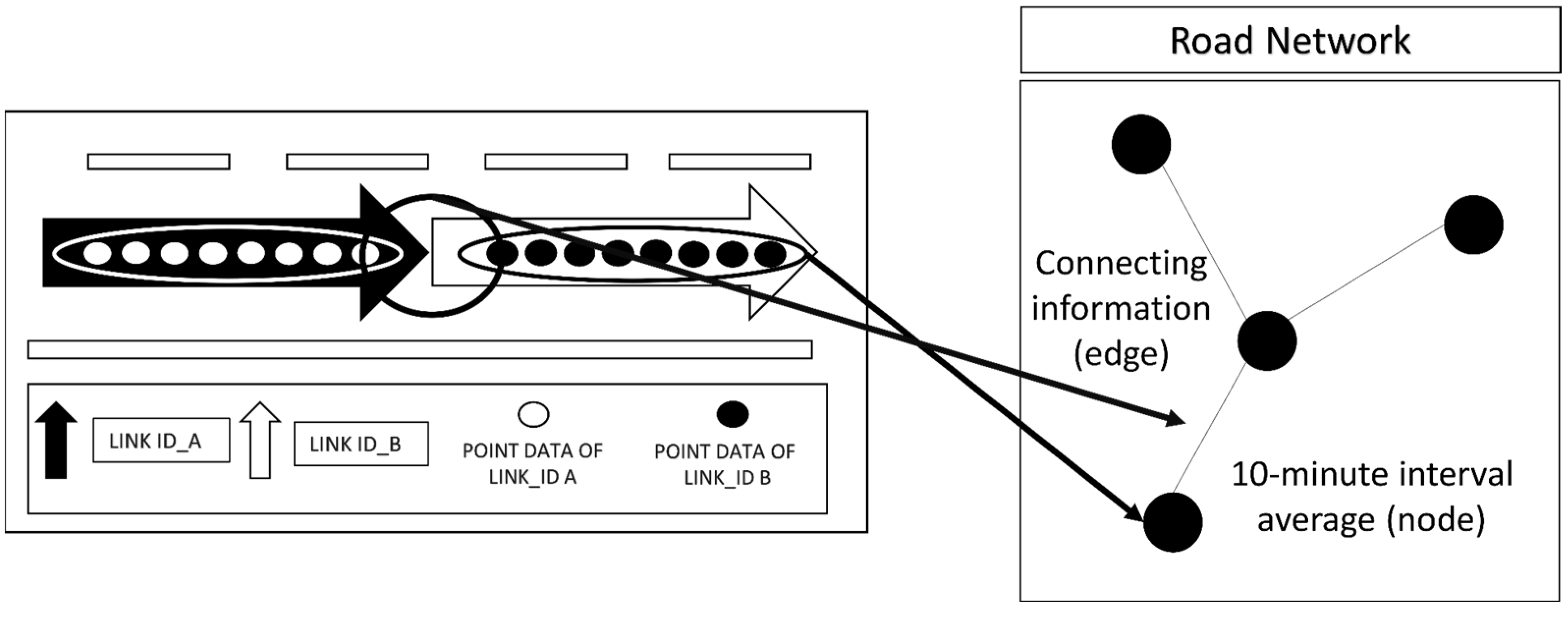Figure 3 depicts the spatial join process linking the point data with the road link data. Each point data can obtain a link index through the spatial join. This data fusion was essential for creating the foundation for further deep learning techniques employed in this study, such as STGCN and CNN.

In summary, the spatial join process played a pivotal role in integrating various data sources and facilitating the creation of graph and image data, which were then harnessed for training deep learning models in this study. This approach enriched the dataset and laid the foundation for the successful exploration of spatio-temporal patterns in the context of road networks and taxi location information.

3.3. Graph Transformation

The graph transformation process involves creating a graph representation using the ‘from node’ and ‘to node’ attributes of the road links. This allows for modeling traffic flow and connectivity between different parts of the road network. Additionally, the data were structured to generate image data, which were based on the properties of the road links and included a time index. These image and graph data representations played a crucial role in capturing the spatio-temporal patterns in the data and were integral to training the STGCN and CNN models.

In this study, generating graphs was a fundamental step in representing the essential dimensions of speed, time, and space for training STGCN, a GCN-based model. GCN-based models rely on graph data for their training and analysis. To create these graph data, we employed a method in which the average value of point data sharing the same link index was assigned as the node value within the graph. The connection information for each link was designated as the edge information of the graph. The outcome of this process was a graph representation of spatio-temporal attributes. Figure 4 visually depicts how graph data were defined for model training.

Several considerations exist regarding the number of links and other parameters in our graph transformation process. One limitation is that an excessive number of links can increase the computational complexity and memory usage, potentially impacting model performance and training time. Conversely, too few links might result in an oversimplified graph that fails to capture the necessary details of the road network. Therefore, in this study’s experiments, we used link data located on main roads in urban areas, where appropriate traffic volume could be collected.

Other important parameters include temporal resolution, which impacts the granularity of the temporal patterns captured and may require more computational resources at higher resolutions and feature selection, where the properties of road links, such as traffic speed, TSR, and brake data, must be carefully chosen to accurately reflect the road network environment and driver intentions. Therefore, this study conducted experiments reflecting various time resolutions, such as 60, 70, 80, and 90 min, and selected data on speed, TSR, and brake information to reflect the road environment and the driver’s intentions.

Each node within the graph was determined by aggregating and averaging the point data over a 10 min window for a given link index. The averaged data served as the feature matrix for STGCN operation. The edges of the graph contained connection information for every node. This connection information was utilized to create an adjacency matrix, which was employed to update the state of each node in a manner consistent with the Laplacian matrix. These graph-based representations were essential for training the GCN-based models as they effectively encapsulated the dynamics and relationships of the network.

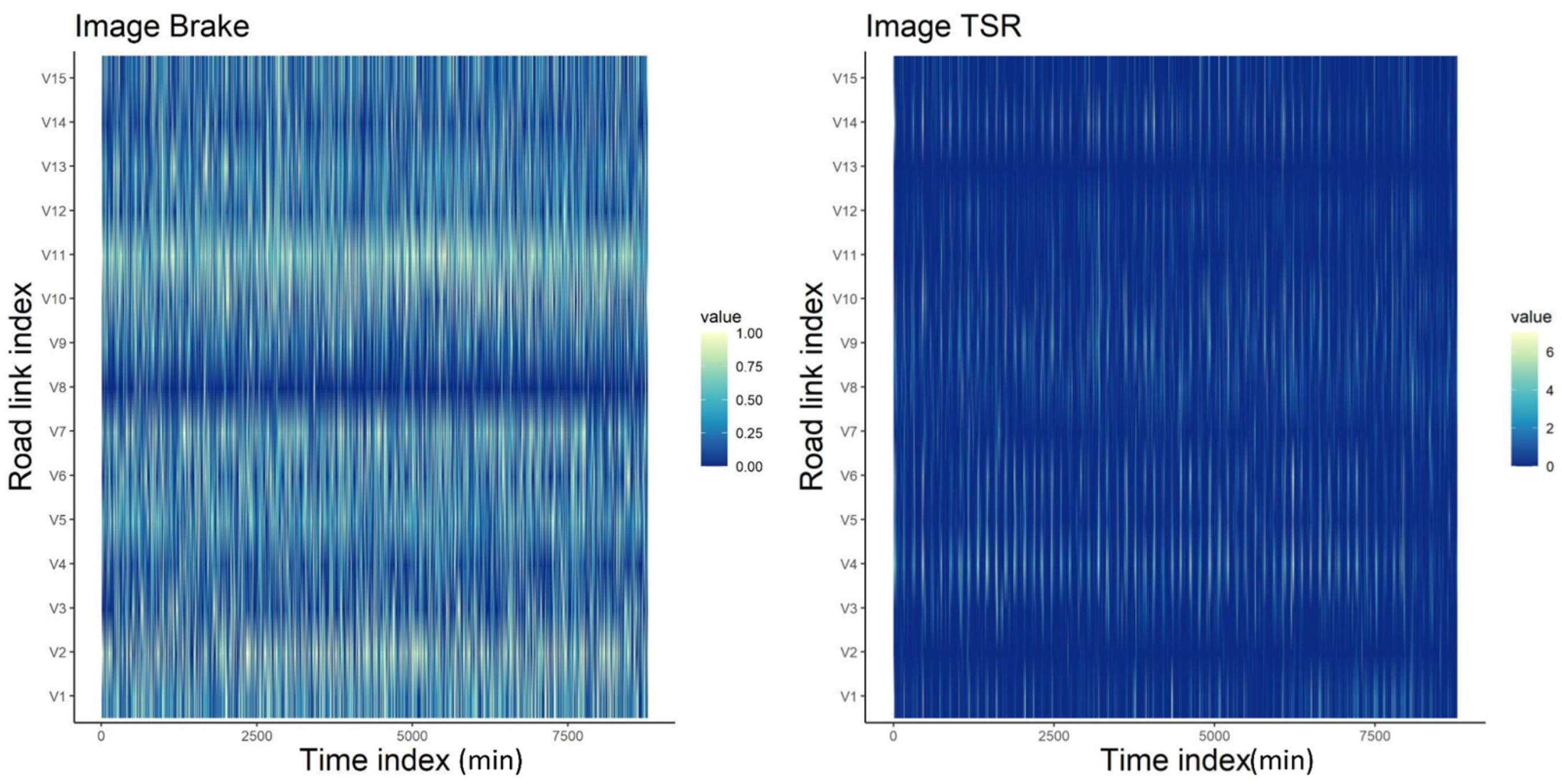
Additionally, this study also transformed the data into images utilized in CNN models. This conversion process bears similarities to the generation of graph data. The images were structured along two axes: time and node index. Figure 5 illustrates the nature of these converted images from brake and TSR information. For example, the X-axis indicates time (min), whereas the Y-axis indicates node index. The color of the images indicates the value of brake and TSR.

This research applied a dual approach, creating graph data for GCN-based model learning and image data for CNN-based model learning. These representations were derived from the same dataset but catered to different deep learning models. The graph data captured the dynamics and connectivity of the network. In contrast, the image data offered a structured representation for analyzing spatio-temporal patterns in the context of the data of the study, thus contributing to a comprehensive and multi-faceted analysis of the road network and taxi location information.

3.4. Short-Term Traffic Speed Prediction Models

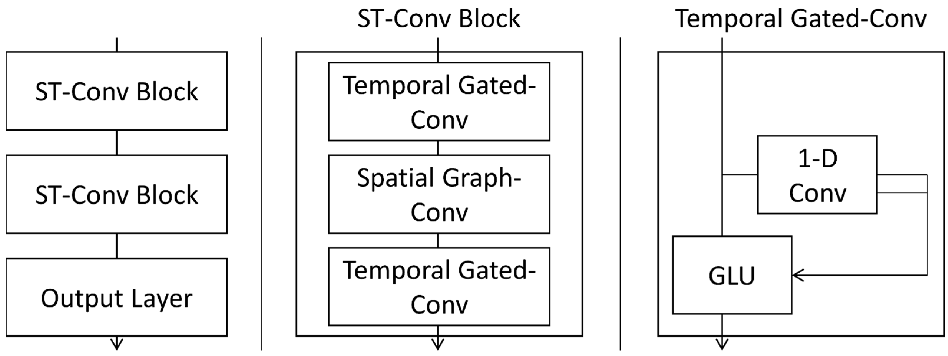
The methods used in this study are STGCN and CNN. STGCN was applied to deal with spatio-temporal and graph-based information. The STGCN used in this study consists of two ST-conv blocks, and one ST-Conv block consists of two temporal gated-conv layers and one spatial graph-conv layer. The architectures of STGCN and the temporal gated-conv layer are shown in Figure 6 [50].

As illustrated in Figure 6, STGCN consists only of convolutional layers. However, CNN cannot deliver long-term dependency because it simply looks at the currently entered image. Generally, it is imperative to consider the previous state for predicting time-series data. Therefore, it has been customary for models used primarily to predict time-series data to use RNN-based models that can learn sequences. STGCN uses the temporal gated-conv layer to learn temporal features with CNN-based models.

The temporal gated-conv layer consists of a 1D-conv and gated linear unit (GLU) [51]. GLU was first introduced by presenting a method based on CNN in language modeling, where RNN was initially dominant. It has long-term dependencies such as LSTM by extracting hierarchical features. The performance was better than that of the existing RNN method and had less computation. The temporal gated-conv layer of STGCN to which this GLU is applied expresses the data as a vector through 1D-conv. We applied the sigmoid function to half of the vector and determined the weight of the vector sequence by the elementwise product with the other half. Finally, by adding the input, GLU was generated as a form of residual learning. The following equation can express a temporal gated-conv:

$$\Gamma *\tau Y=P\odot \sigma \left(Q\right)\in {ℝ}^{M-K_t+1\times C_0},$$

(1)

where a three-dimensional variable can be generated using the convolution kernel $\Gamma$ equally for all nodes $Y$. $P$ and $Q$ represent each half of the vectors converted into 1D vectors, $M$ represents the size of the time step to be considered, $K_t$ represents the kernel size of the temporal convolution, and $C_O$ represents the channel size.

In this study, the kernel size was determined to be 3 through the grid search, and the time step to be considered was 12, which means 120 min. STGCN, which learns temporal features through the temporal gated-conv layer, uses the spatial graph-conv layer to reflect the spatial features. However, the convolution operation cannot be applied directly to the graph. As a solution, STGCN employs spectral graph convolution to apply a convolution operation to the graph data. Spectral graph convolution performs convolution operations using Fourier transform used in signal processing. Graph Fourier basis $U\in {ℝ}^{n\times n}$ is the matrix of eigenvectors of the normalized graph Laplacian $ℒ$, defined as follows:

$$ℒ=I_n-D^{-\frac{1}{2}} \widehat{A}{D}^{-\frac{1}{2}}=U\Lambda U^T\in {ℝ}^{n\times n},$$

(2)

where $I_n$ is an identity matrix, $D$ is the diagonal degree matrix, and $A$denotes the weighted adjacency matrix.

The spatial graph-conv layer performs spectral graph convolution by reshaping data that have passed through the temporal gated-conv layer. The spatial graph-conv layer updates the status of the current node with information from the peripheral nodes and is performed via the Laplacian matrix. Multiplying the Laplacian matrix by the feature matrix of the node provides the difference between the node and neighboring node for the feature. The notion of the spectral graph convolution operator ‘$*\mathcal{G}$’ is defined as the multiplication of a signal $x\in {ℝ}^n$ with a kernel $\Theta$.

$$\Theta *\mathcal{G}x=\Theta (ℒ)x=\Theta \left(U\Lambda U^T\right)xs=U\Theta \left(\Lambda \right)U^{T}x,$$

(3)

It requires a substantial computational cost, such as $\Theta$. To alleviate this problem, one study [52] developed a localized technique to reduce the number of parameters of spectral graph convolution.

$$\Theta *\mathcal{G}x=\Theta (ℒ)x\approx {{\displaystyle \sum }}_{k=0}^{\mathcal{K}-1}{\theta }_{\mathcal{K}}{P}_{\mathcal{K}}\left(\widehat{ℒ}\right)x,$$

(4)

where $P_k\left(\widehat{ℒ}\right)$represents a Chebyshev polynomial of order k evaluated on the scaled Laplacian. $\widehat{ℒ}=2ℒ/{\lambda }_{max}-I_n$, $\theta \in {ℝ}^{\mathcal{K}},$ and ${\lambda }_{max}$ denote the vector of polynomial coefficients, kernel size of the graph convolution, and the maximum eigenvalue of $ℒ$, respectively.

STGCN constructs ST-conv blocks that deal with temporal and spatial features through temporal gated-conv and spatial graph-conv. The sandwich structure comprises two temporal gated-convs with a spatial graph-conv in between and supports bottleneck strategies through upscaling and downscaling of the channels. Dropout and batch normalization were involved in mitigating overfitting. The output for the input $v$ follows the equation:

$$v^{l+1}={\Gamma }_1^l*\tau ReLU\left({\Theta }^l{*}_{\mathcal{G}}\left({\Gamma }_0^l*\tau v^l\right)\right),$$

(5)

where $v$ is an observation vector, ${\Gamma }_0^l$ and ${\Gamma }_1^l$ are the upper and lower temporal kernel within block $l$, respectively, and ${\Theta }^l$ is the spectral kernel of graph convolution.

In this study, we used speed data as a feature matrix. Moreover, the brake and TSR data were learnt in the same structure and then concatenated to observe the change in performance. The other deep learning method, CNN, was trained with the same data and observed the performance change to find the appropriate data for each method. Unlike STGCN, the CNN model, which learns image data consisting of time and node indexes as an axis, extracts the feature of the data as a combination of convolutional and pooling layers. The output of the model is calculated using the following formula:

$$o_i=pool\left(ReLU\left(W_i{x}_i+b_i\right)\right),$$

(6)

where $pool$ denotes average pooling, and $i$ denotes the depth of CNN.

We used a simple CNN structure owing to the relatively high computational cost, and there was no significant change in performance when using a model with many layers, such as ResNet, called the revolution of depth.

Traffic speed, brake, and TSR data acquired from urban road networks were learnt using CNN and STGCN models. To develop a model with optimal performance, we observed which data could have the highest performance when applied to various model learning. In this study, we found that the best performance is to learn TSR and brake data that could reflect the intention of the driver and road environment by CNN and traffic speed data by STGCN. We defined a hybrid model by converging the two models based on the results of the experiment. The architecture of the model derived through this study is shown in Figure 7.

After the feature extraction was achieved using the presented STGCN and CNN model, the weights for each feature were learned with a multi-layer perceptron. For learning, we used 80% (49 days) of the total data, with 10% (6 days) used for validation, 10% used for testing, and the batch size set to 256.

For model evaluation, we used mean absolute error (MAE) and root mean square deviation (RMSE), as follows:

$$MAE=\frac{{{\displaystyle \sum }}_{i=1}^n\left|y_i-x_i\right|}{n},$$

(7)

$$RMSE=\sqrt{\frac{1}{n}{{\displaystyle \sum }}_{i=1}^n{\left(x_i-y_i\right)}^2},$$

(8)

where $n$denotes the number of samples, $y$ denotes the ground truth, and $x$ denotes the predicted value.

RMSE is a root form of mean square error (MSE). MSE squares the difference between the predicted and target values, and those features cause some issues. MSE is sensitive to outliers. If the error is between 0 and 1, it reflects as smaller than the original; if the error is greater than 1, it reflects as larger than the original. RMSE can solve MSE problems to some extent. As MAE takes absolute values, it has a characteristic that it is relatively not affected by the outlier compared to MSE and RMSE.

4. Experimental Results

In this study, we integrated STGCN and CNN models to predict the traffic speed of the road network in network units. Predictions were made by reflecting the environment constituting the road network and the intention of the drivers. Thus, this study used speed, TSR, and brake information. Furthermore, we compared the performance of the proposed model with that of the existing methods. The baseline models were STGCN and CNN. We compared the accuracy by considering a combination of all the variables and methods.

In terms of the experimental environments, all methods were coded in Python. Experiments were conducted on a computer with an NVIDIA GeForce RTX 3080 GPU and 10 GB of memory.

Table 2. Parameters used in this case study.

Parameter	Value
CNN layers	3
STGCN layers	2
Convolution kernel size	3
Time step	60–90
Number of hidden units	625
Graph convolution kernel size	3

indicates the parameters used in this study.

To improve the performance of deep learning models and to find the optimal model configuration, various hyperparameters must be adjusted. Hyperparameters affect the model training process. Thus, it is vital to set them correctly. The hyperparameter tuning process involves experimentally adjusting various settings, such as the learning rate of the model, mini-batch size, dropout rate, etc., to find the best combination.

Currently, Grid Search is widely used because it helps systematically search for combinations of multiple hyperparameters. Grid Search generates all possible combinations of hyperparameters of interest in a predefined grid, learns a model for each combination, and evaluates performance. Through these iterative experiments, we find the best hyperparameter combination. This process is an essential step to optimize model performance and prevent overfitting. Grid Search allows one to perform the hyperparameter tuning process systematically and helps to find the best model settings; therefore, we used Grid Search to tune our hyperparameters. The epoch was set to 200. If the validation loss did not improve at all during the training process, the training process was stopped even though the epoch is more than 100 times. The batch size was 256, learning rate was 0.001, dropout probability was 0.5, and the optimizer was Adam.

In the experiments, we conducted multi-step speed prediction of the road network at several time steps, including 60 min, 70 min, 80 min, and 90 min. STGCN, CNN, and the proposed model were all trained using speed, brake, and TSR data.

The experimental results confirmed that the proposed model showed the best performance in all time step intervals. Specifically, the proposed hybrid model, which integrates STGCN and CNN, outperformed the individual STGCN and CNN models. This suggests that the hybrid model can capture both spatial and temporal dependencies more effectively than the standalone models.

Table 3. Prediction results of MAE and RMSE.

Predictions after n − 1 Time Step (min)	STGCN (Speed, TSR, Brake)		CNN (Speed, TSR, Brake)		STGCN (Speed) + CNN (TSR, Brake)
	MAE	RMSE	MAE	RMSE	MAE	RMSE
60	17.2089	21.009	17.1457	20.8469	17.0332	20.7712
70	17.2459	20.9811	17.1490	20.9015	17.0503	20.7862
80	17.1122	20.8314	17.2566	20.9147	17.1464	20.9856
90	17.2394	20.9632	17.2427	20.9085	17.0812	20.8542

shows that the hybrid model consistently achieved lower MAE and RMSE values across all time steps compared to the individual STGCN and CNN models. This improvement is attributed to the hybrid model’s ability to leverage the strengths of both models: the spatial understanding of CNN and the spatio-temporal processing capability of STGCN. Figure 8 represents the prediction error maps of road links between the predicted speed and the observed speed using MAE. The colors on the map indicate the magnitude of the prediction error at each road link, with different colors representing different ranges of MAE values.

The error distribution shown in Figure 8 indicates that the hybrid model achieves low prediction errors across most road links, demonstrating its effectiveness in capturing the spatio-temporal patterns of traffic speed. The areas with higher prediction errors (yellow and red regions) are relatively sparse, suggesting that while the hybrid model performs well overall, there are specific regions where further improvements could be made. These high-error areas could be due to unique traffic patterns or insufficient data, which the hybrid model may not fully capture.

To confirm whether the results of this experiment are statistically significant, we apply a one-way ANOVA test using MAE and RMSE values of each model. ANOVA testing can indicate whether there are any statistical differences between the means of three or more independent groups. Before conducting an ANOVA test, we assess the assumptions of the ANOVA test. In this study, we apply the Shapiro–Wilk [53] and the Levene tests [54] to assess normality and homoscedasticity. These tests presented that the data did not break the assumptions ($p\text{-}\mathrm{value}>0.05$). Finally, the ANOVA test revealed that there was a statistically significant difference among groups ($F\left(2, 9\right)=6.09, p\text{-}\mathrm{value}<0.05$) for MAE. However, the ANOVA test for RMSE showed no statistically significant differences ($F\left(2, 9\right)=1.68, p\text{-}\mathrm{value}=0.23$).

Additionally, this study conducted post hoc tests for pairwise comparisons that can compare all different combinations of the treatment groups. Tukey’s Honestly Significant Difference (HSD) test revealed that the proposed model showed a statistically significant difference compared with the CNN model ($p\text{-}\mathrm{value}<0.05$). When compared to STGCN, there was also a statistically significant difference ($p\text{-}\mathrm{value}<0.05$). With regard to CNN and STGCN, $p\text{-}\mathrm{value}=0.996$, indicating that there was no statistically significant difference between CNN and STGCN.

Furthermore, we calculated the effect size by dividing the average difference between the two sample groups by the estimated standard deviation. The effect size indicates the similarity between the distributions of the two groups. When the effect size is large, the overlap between the two groups is small. Therefore, the two groups are very different. When the effect size is small, the overlap between the two groups is significant; i.e., the two groups are very similar. The effect size indicates the extent of difference between the groups to be compared. The effect sizes, such as Cohen’s d, between the proposed model and STGCN model, and between the proposed model and CNN model, are 2.207 and 2.201, respectively. Both cases show very large effect sizes. The effect size indicates the practical degree of difference between groups. Therefore, the experimental results demonstrated that the proposed model outperformed alternative models, statistically and practically regarding MAE. In addition, Cohen’s d of RMSE between STGCN and our proposed model was 1.09, which indicates a large effect size. The effect size between CNN and the proposed model indicated a medium effect size (i.e., Cohen’s d = 0.52). Accordingly, although there are no statistically significant differences for RMSE, there are practical differences for RMSE.

Regarding the effect of data, in this study, we investigated the effect of TSR data on traffic speed prediction. We analyzed the effect of TSR data by adding or removing TSR data while constructing the proposed model.

Table 4. Prediction results based on the presence or absence of TSR data.

Predictions after n − 1 Time Step (min)	STGCN (Speed) + CNN (TSR, Brake)		STGCN (Speed) + CNN (Brake)
	MAE	RMSE	MAE	RMSE
60	17.0332	20.7712	17.0403	20.8899
70	17.0503	20.7862	17.2428	20.9741
80	17.1464	20.9856	17.0897	20.9794
90	17.0812	20.8542	17.0721	20.8225

shows the difference between the models with and without TSR.

Based on the results shown in Table 4, we conducted an ANOVA test and calculated the effect size. The results of the ANOVA test showed that there was no statistically significant difference ($F\left(1, 6\right)=0.42, p\text{-}\mathrm{value}=$0.54). Cohen’s d was approximately $0.4596 \cong 0.5.$This effect size is approximately medium. The results of the ANOVA test based on RMSE also indicated no statistically significant difference $\left(F\left(1,6\right)=1.18, p\text{-}\mathrm{value}=0.317\right)$. However, unlike the result of MAE, the effect size for RMSE, such as Cohen’s d, was 0.771. This effect size is medium. Although there was no statistically significant difference between the presence and absence of TSR, practical significance, such as Cohen’s d, presented that the effect was sufficient to be meaningful in the real world. Therefore, using TSR can improve the performance of the model.

5. Discussion and Conclusions

In this study, we presented a hybrid model for a deeper understanding of road infrastructure, which is growing in size and importance with the development of urban areas. The hybrid model predicts the traffic speed for road networks that are affected by various variables and have a complex structure in which states constantly change. The model presented in this study is a fusion of STGCN and CNN, which reflects spatio-temporal features and considers graph-based relationship features to make predictions. Additionally, the features for the models were extracted from TSR and brake data to reflect the intention of the driver.

The experimental results demonstrated that the proposed model outperformed the STGCN and CNN models for traffic speed prediction. There are statistically significant differences between the proposed model and the alternative models using MAE. Furthermore, there was a large effect size between the proposed model and others. Therefore, it seems reasonable to conclude that using the proposed model is more effective statistically and practically than using alternative models, such as STGCN and CNN.

In previous studies, STGCN- and CNN-based models showed better performance by reflecting multiple factors compared to RNN-based models, which actually have difficulty reflecting time series with multiple factors. CNN-based models are suitable for parallel processing, can perform tasks quickly, and cannot be significantly affected by sequence length, unlike RNN-based models. STGCN is also specialized in processing data in a graph and is suitable for analyzing transportation networks that represent relationships between nodes. Like CNN, it is suitable for parallel processing and allows complex models to be handled more efficiently than RNN, which proceeds sequentially. Furthermore, unlike CNN, STGCN can have long-term dependency through GLU. This can positively affect prediction performance if it is time-dependent and shows some degree of correlation. However, the prediction performance can be decreased when the temporal correlation is very low. Therefore, it is essential to consider whether the data fit with the selected model. In that context, the hybrid model proposed in this study was appropriate and generated optimal predictions according to the characteristics and data of each model.

Moreover, we investigated the effect of data, such as TSR. We applied TSR to the proposed model and removed it from the proposed model. While there were no statistically significant differences between the models, there was a medium effect size. Therefore, the model with TSR practically performed better than the model without TSR.

In summary, we proposed a hybrid model based on STGCN and CNN. The structure of the proposed model uses graph data and image data together. We used STGCN to train speed data and CNN to train TSR and brake information. Additionally, this study utilized TSR data collected from Mobileye sensors to reflect the intention of the driver for traffic speed prediction.

The results of this study are expected to provide a deep understanding and insight into the traffic flow on road networks, which plays a vital role in developing cities. This is expected to contribute to the efficient operation and improvement of transportation networks, reduce unnecessary fuel combustion, and have a positive impact on environmental, economic, and time costs. However, we used Grid Search to find the optimal hyperparameters, which has the disadvantage of consuming considerable cost and time. In the future, we plan to research how to save on cost and time for optimizing hyperparameter settings over a wider area. Future research could enhance the proposed model by incorporating additional data sources such as real-time traffic incidents and weather forecasts, ensuring scalability on more extensive road networks, thereby improving urban traffic management and reducing congestion.