Optimization Research of Heterogeneous 2D-Parallel Lattice Boltzmann Method Based on Deep Computing Unit

Abstract

Currently, research on the lattice Boltzmann method mainly focuses on its numerical simulation and applications, and there is an increasing demand for large-scale simulations in practical scenarios. In response to this situation, this study successfully implemented a large-scale heterogeneous parallel algorithm for the lattice Boltzmann method using OpenMP, MPI, Pthread, and OpenCL parallel technologies on the “Dongfang” supercomputer system. The accuracy and effectiveness of this algorithm were verified through the lid-driven cavity flow simulation. The paper focused on optimizing the algorithm in four aspects: Firstly, non-blocking communication was employed to overlap communication and computation, thereby improving parallel efficiency. Secondly, high-speed shared memory was utilized to enhance memory access performance and reduce latency. Thirdly, a balanced computation between the central processing unit and the accelerator was achieved through proper task partitioning and load-balancing strategies. Lastly, memory access efficiency was improved by adjusting the memory layout. Performance testing demonstrated that the optimized algorithm exhibited improved parallel efficiency and scalability, with computational performance that is 4 times greater than before optimization and 20 times that of a 32-core CPU.

1. Introduction

The lattice Boltzmann method (LBM) is a computational fluid dynamics (CFD) simulation method that is derived from the theory of molecular motion. It divides the fluid domain into regular grids and simulates the flow and collision of particles on these grids to model the behavior of the fluid [1]. Compared to traditional CFD methods, LBM has the advantage of being easy to implement and parallelize while also being capable of handling complex boundaries and irregular structures. As a result, LBM has been widely applied in various theoretical studies and engineering practices [2,3,4].

With the continuous development of CFD research and applications, the complexity of the problems, grid sizes, and solution accuracy are constantly increasing, which poses an urgent demand for large-scale parallel CFD simulations [5]. As Moore’s Law gradually loses its effectiveness, heterogeneous computing architectures have become the mainstream trend in the field of high-performance computing [6] and are widely used in scientific research, engineering simulations, artificial intelligence [7], and big data analysis, among other fields. In recent years, the rapid development of accelerators such as GPUs, DCUs (Deep Computing Units), and FPGAs has made the “CPU + accelerator” architecture widely adopted in heterogeneous high-performance computers. In order to fully utilize the performance of heterogeneous high-performance computers, it is necessary to develop heterogeneous parallel applications using parallel models. Such as the popular CUDA heterogeneous parallel programming model [8]. However, CUDA can only be used on NVIDIA GPUs. Due to the diversity of heterogeneous computing architectures, different accelerators support different programming models. Therefore, applications need to be ported and optimized for different heterogeneous platforms, which greatly increases the difficulty of developing and optimizing heterogeneous parallel applications. In recent years, a series of cross-platform, parallel programming models have been proposed by academia and industry that support developers using a set of code to generate executable files that can run on different architectures. For example, the general-purpose heterogeneous programming language OpenCL [9] abstracts hardware into a unified platform model [10], while OpenACC [11] adds directive statements to C or Fortran code to identify the location of parallel code regions [12]. Parallel programming frameworks such as Kokkos [13] and RAJA [14] are based on C++ template metaprogramming techniques, providing a unified interface for describing data and parallel structures, with specific implementations supported by the framework software at the lower level [15]. With the development of these cross-platform parallel programming models, developers can more conveniently develop and optimize heterogeneous parallel applications on different hardware platforms, thus better utilizing the potential of heterogeneous high-performance computers. This will drive research and applications in fields such as CFD towards higher performance and efficiency.

In recent years, many researchers have been devoted to the heterogeneous parallelization and performance optimization of LBM simulations on heterogeneous supercomputers. Tölke [16] designed a D2Q9 SRT-LBM method on a single GPU, using shared memory to reduce the number of global memory reads and writes to reduce memory access time. With the improvement of GPU hardware performance, Obrecht et al. [17] found that the impact of aligned memory access time is no longer important for GPU algorithms in LBM. They proposed two schemes, Split and Revise, that utilize shared memory. Zhou et al. [18] introduced surface boundary handling in the GPU algorithm of LBM and provided implementation details for boundary treatment. Lin et al. [19] implemented the mapping of the Multi-Relaxation-Time LBM method on a single GPU. Their experiments showed a 20.4× speedup compared to the CPU implementation of the same algorithm. To achieve larger-scale computations, algorithms in multi-GPU heterogeneous environments have received more attention. Wang et al. [20] utilized the characteristics of multi-stream processors to achieve large-scale parallel computing in multi-GPU environments by hiding the communication time between the CPU and GPU. Subsequently, Obrecht et al. [21] further partitioned the computational grid using MPI parallelism to solve larger-scale grids with multiple GPUs.

Feichtinger et al. [22] implemented heterogeneous parallel acceleration of LBM on the Tsubame 2.0 supercomputer using GPUs and tested strong and weak scalability with more than 1000 GPUs. Li et al. [23] implemented and optimized the LBM open-source code openLBMflow on the Tianhe-2 supercomputer using the Intel Xeon Phi coprocessor (MIC) for acceleration. Scalability tests were conducted using 2048 nodes. Liu et al. [24] developed a complete LBM software, SunwayLB, on the Sunway TaihuLight supercomputer cluster, covering the entire process from preprocessing to computation. Its acceleration performance is up to 137 times faster, making large-scale industrial applications and real-time simulations of LBM possible. Riesinger et al. [25] implemented a fully scalable LBM method for CPU/GPU heterogeneous clusters. They used the Piz Daint CPU/GPU heterogeneous cluster with 24,576 CPU cores and 2048 GPU cards, achieving a grid size of up to 680 million. Watanabe et al. [26] simulations have demonstrated good weak scaling up to 16,384 nodes and achieved a high performance of 10.9 PFLOPS in single precision. Xia et al. [27] proposed a parallel DEM-IMB-LBM framework based on the Message Passing Interface (MPI). This framework employs a static domain decomposition scheme, partitioning the entire computational domain into multiple subdomains according to predefined processors. The framework was then applied to simulation scenarios of multi-particle deposition and submarine landslides. In addition, many scholars have conducted parallel studies on various applications of the LBM [28,29,30,31,32,33].

This paper implements a multi-node, multi-DCU heterogeneous parallel framework on the “Dongfang” supercomputing system. This framework’s design differs from those of other researchers and demonstrates good parallel efficiency, which can provide a valuable reference for other researchers. Although the manuscript primarily reports 2D simulation results, we believe that the use of the hardware and its performance optimization still hold innovation and reference value. In this study, the correctness and effectiveness of the LBM heterogeneous parallel algorithm were validated through lid-driven cavity flow using the D2Q9 model of the single relaxation time LBM. Subsequently, optimization and performance testing were conducted, resulting in a parallel efficiency of over 90%. The following aspects were primarily focused on:

Firstly, a heterogeneous parallel algorithm for LBM was implemented using the cross-platform parallel programming model OpenCL. This implementation enables LBM simulations to be executed in parallel on various computing hardware, effectively utilizing the computational resources of different architectures.

Secondly, to reduce the communication overhead on the CPU side and the memory access overhead on the DCU side, some optimization strategies, such as non-blocking communication, utilization of high-speed shared memory, and coalesced access, were adopted. These strategies effectively manage data transmission and memory access.

Finally, the performance testing demonstrates that by adjusting the computational grid size on the CPU to be 1/10 of that on a single DCU, a computational balance between the CPU and DCU can be achieved. This adjustment allows the computation time on the CPU and DCU to overlap, fully utilizing the available computational resources.

2. Numerical Methods

In this study, the D2Q9 model is used, where the velocity components are distributed, as shown in Figure 1.

LBM originated from lattice gas automata and can be derived from the macroscopic Navier–Stokes equations through the Chapman–Enskog multiscale expansion. The control equations and computational methods of the standard LBM are relatively simple. The equations are as follows:

$$f_i(x+c_i\delta t,t+\delta t)=f_i(x,t)+\Omega \left(f\right)$$

(1)

$f_i(x,\mathrm{t})$ represents the velocity distribution function at time $t$ at spatial grid point x, $c_i$ is the discrete velocity set of fluid particles, $\delta t$ is the discrete time step, t is the current time step, and $\Omega \left(f\right)$ is the collision operator. The single relaxation time LBM model is adopted, and the equation is as follows:

$$f_i(x+c_i\delta t,t+\delta t)-f_i(x,t)=-\frac{1}{\tau }\left[f_i(x,t)-f_i^{eq}(x,t)\right]$$

(2)

$\tau$ is the relaxation factor, and $f_i^{eq}(x,t)$ is the equilibrium distribution function. For the D2Q9 discrete model, the equilibrium distribution function is as follows:

$$f_i^{eq}=\rho {\omega }_i\left[1+\frac{c_i\cdot u}{c_s^2}+\frac{(c_i\cdot u{)}^2}{2c_s^4}-\frac{u^2}{2c_s^2}\right]$$

(3)

The weight coefficient is ${\omega }_i$, the dimensionless speed of sound is $c_s=c/\sqrt{3}$, and the lattice velocity is $c=\delta x/\delta t$, where $\delta x$ and $\delta t$ are the lattice spacing and time step. The weight coefficients and discrete velocities for the 9 directions are shown in

Table 1. Parameters of the D2Q9 model.

Model	Velocity Component	Quantity	Mould Length	Weight
D2Q9	(0, 0)	1	0	4/9
	(±1, 0)	2	1	1/9
	(0, ±1)	2	1	1/9
	(±1, ±1)	4	$\sqrt{2}$	1/36

.

The macroscopic density and velocity of the fluid in the lattice Boltzmann equation are obtained from Equations (4) and (5), respectively:

$$\rho =\sum _i{f}_i=\sum _i{f}_i^{eq}$$

(4)

$$\rho u=\sum _i{c}_i{f}_i=\sum _i{c}_i{f}_i^{eq}$$

(5)

The relationship between the viscosity coefficient $\gamma$ and the relaxation time $\tau$ can be expressed as:

$$\gamma =(\tau -\frac{1}{2})c_s^2\delta t$$

(6)

During the simulation process, the periodic grid is treated as a normal internal grid, while the solid boundaries are handled using the standard bounce-back rule. As shown in Figure 2, the arrows represent the components of the distribution function in different directions. It can be observed that at the solid boundary, the outward components of the distribution function are completely reversed to simulate the bouncing effect on the solid surface, while the remaining components migrate to the adjacent lattice points to maintain the continuity of the flow field.

3. Heterogeneous Parallel Implementation

3.1. Description and Advantages of DCU Architecture

A DCU (Deep Computing Unit) is a specially designed accelerator card used for heterogeneous computing. It connects to the CPU via the PCI-E bus and aims to enhance computational performance, particularly for computation-intensive program modules or functions. The DCU operates independently of the CPU, featuring its own processor, memory controller, and thread scheduler, enabling it to function as an autonomous computing system.

The system architecture of the DCU includes the data pathway (DMA) between the CPU and DCU, compute unit arrays (CU), a multilevel cache system (including Level 1 and Level 2 caches), and global memory. Inside the DCU, there are multiple compute unit arrays, with each compute unit (CU) consisting of four SIMD units. Each SIMD unit includes multiple stream processing units responsible for performing basic arithmetic operations such as addition, subtraction, and multiplication. These stream processing units are highly optimized for high-speed data processing and parallel computing, greatly enhancing the processor’s computational efficiency. Its streamlined and efficient instruction set enables the DCU to effectively accelerate computational processes in various computation-intensive scientific and engineering applications, making it a vital tool for enhancing processing capabilities.

Advantages of DCU Architecture Compared to Existing Exascale Architectures: The DCU architecture uses the latest 7 nm FinFET technology and is designed based on microarchitecture for large-scale parallel computing. It not only has powerful double-precision floating-point computation capabilities but also excels in single-precision, half-precision, and integer computations. It is the only acceleration computing chip in China that supports both full-precision and half-precision training.

3.2. Parallel Feasibility Analysis of LBM

When using the D2Q9 model, each particle’s velocity update depends solely on the values of its nine neighboring particles. In this discrete approach, a particle’s value can be temporarily stored until all particles are computed. Consequently, the update of one particle does not affect others that have not been updated yet. This makes the method well-suited for parallel computing in flow field calculations.

3.3. Multi-Node Parallel Algorithm Implementation

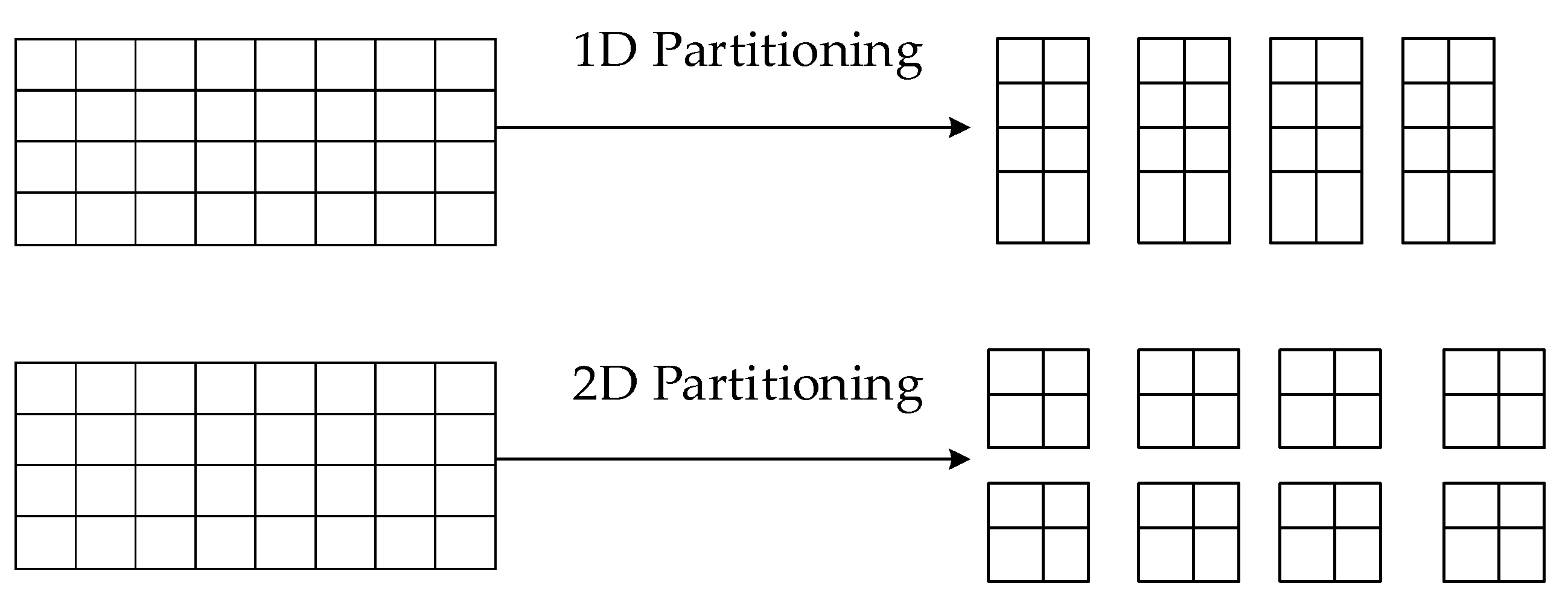
In LBM simulations using MPI, the domain is typically partitioned using a domain decomposition approach. For the D2Q9 model in a 2D computational domain, two types of partitioning can be used: 1D and 2D partitioning. The schematic diagrams of these partitioning approaches are shown in Figure 3. This domain partitioning method divides the computational domain into multiple subdomains, with each subdomain assigned to a node.

Experimental tests showed that the time overhead of one-dimensional and two-dimensional partitions is about the same. For some simple simulation problems, one-dimensional partitioning can handle data more efficiently. One-dimensional partitioning requires storing relatively less data, saving memory space during large-scale simulations, and reducing communication overhead between a large number of nodes.

This paper employs a 1D partitioning approach for a 2D computational domain, where the model is divided along the x-axis to distribute the lattice evenly among multiple processes in the communication domain.

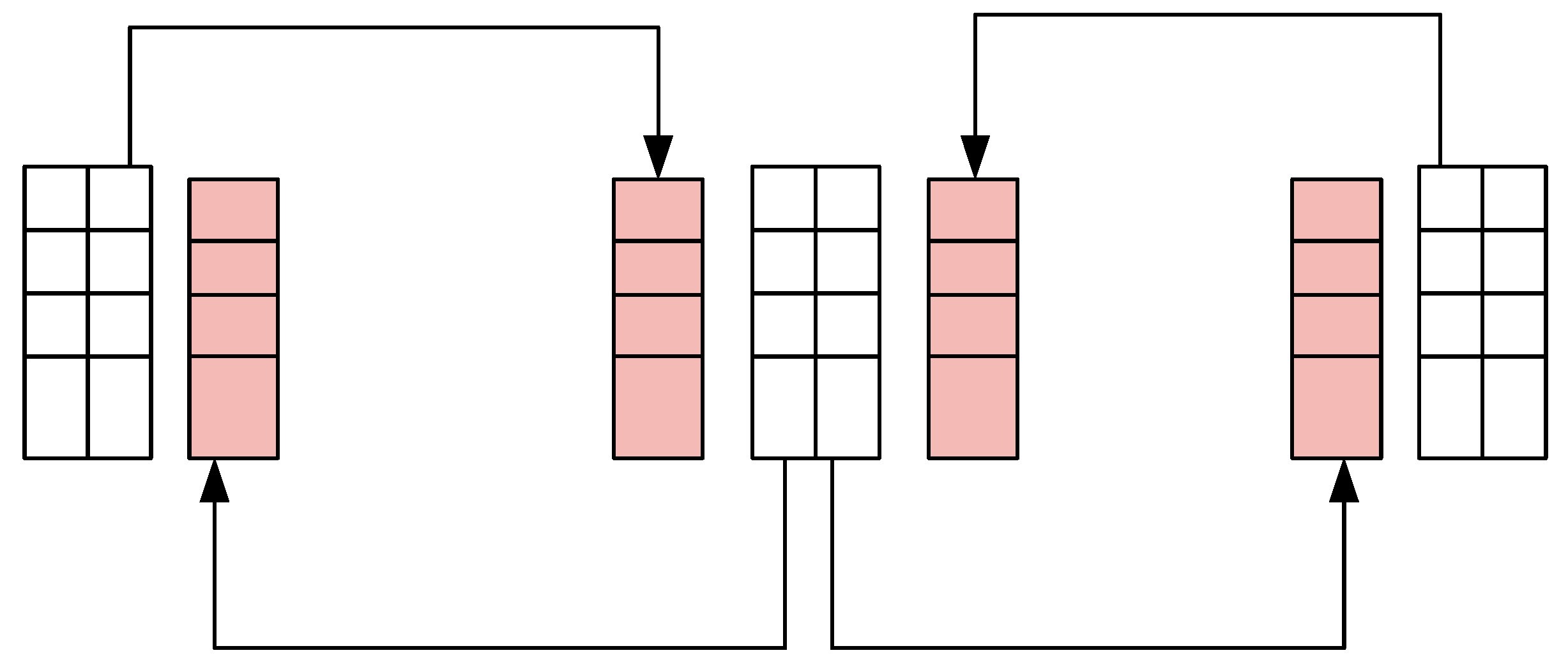
During the flow process in the LBM method, the lattice on the boundaries of the computational domain requires information about the distribution functions of the neighboring lattice. This necessitates data communication to obtain the relevant information from neighboring lattices. Therefore, an additional layer of virtual boundaries is added outside the boundaries of each computational region involved in data communication. These virtual boundaries are used to store the relevant information about the boundary lattice from neighboring nodes, facilitating data communication.

Figure 4 illustrates a schematic diagram of 2D communication. The shaded regions represent data buffer zones, and the arrows indicate communication. The main purpose is to transmit the distribution function values from the boundaries of each sub-grid to the buffer zones of neighboring grids. As a result, each node needs to perform four communication operations.

3.4. Multi-Node and Multi-DCU Parallel Algorithm Implementation

When performing collision and flow calculations involving particle distribution functions, it is crucial to address the issue of data overwriting. This is because, after the collision, the particle distribution functions of each lattice will flow to the neighboring lattice, updating their particle distribution functions. However, when the neighboring lattice performs collision and flow calculations, it may use the particle distribution functions of the next iteration step instead of the current one. To avoid this problem, a dual-grid mode is adopted in this paper. In the dual-grid mode, an additional array of the same size as the original particle distribution function array is allocated during flow field initialization. When the lattice in the flow field performs collision and flow operations, it first reads data from the original particle distribution function array for collision calculations. Then, they store the collision results in the additionally allocated array. After all lattices have completed this step, the pointers of the two arrays are swapped, completing the flow operation. In this way, the original array contains the updated particle distribution function data for the current time step.

When performing parallel computations using DCU, data transfer is often the most time-consuming part of the computation process. Therefore, designing an efficient data transfer strategy can greatly improve computational efficiency. In this paper, a struct array is used to store data on the CPU. The struct consists of particle density, horizontal velocity, vertical velocity, particle distribution functions, and temporary particle distribution functions. Each lattice stores such a struct, making the entire grid a large struct array. During data transfer, an address mapping technique is used to efficiently locate the grid data that each DCU needs to compute based on the base address and the offset. Then, the data are transferred from the host side to the device side based on their length. This transfer method allows for the completion of data transfer with just one call to the clEnqueueWriteBuffer function for each iteration of computation.

In the implementation of the multi-DCU algorithm, the calculation domain is divided, and each subdomain is assigned to the corresponding DCU to perform the computation. Typically, the entire domain is divided into multiple equally sized blocks to achieve load balancing among the DCUs. This paper adopts a one-dimensional partitioning approach, where each DCU calculates a portion of the domain.

During the particle flow process, particles on the boundary grids of a DCU will flow to the neighboring boundary grids of other DCUs. Therefore, this paper addresses two scenarios: multiple DCUs on the same node and multiple DCUs on different nodes. For multiple DCUs on the same node, the grid size of each DCU is expanded outward. An additional layer of grid values is added after the flow is read and computed, allowing the particle data of the edge grids to be accessed by neighboring DCUs. This ensures the update of distribution functions on the edge grids during the flow process. For multiple DCUs on different nodes, a virtual boundary layer is added to the computation boundaries of each node. This virtual boundary layer is used to store the relevant information on the boundary grids of neighboring nodes. The computed data of each DCU are transferred from the device side to the host side. Then, using MPI, the host-side grid information is exchanged among the nodes to enable communication between multiple nodes and multiple DCUs.

3.5. Heterogeneous Parallelization Implementation Based on OpenMP, MPI, Pthreads, and OpenCL

The computational resources used in this study are derived from the domestically developed advanced supercomputing platform “Dongfang” supercomputer system. This system employs a “CPU + DCU” heterogeneous architecture and consists of thousands of nodes. Each node is equipped with a domestically developed 32-core processor, 128 GB memory, and 4 DCU accelerator cards. Each DCU is equipped with 16 GB memory, a bandwidth of 1 TB/s, and a mounted shared storage system.

Figure 5 illustrates the heterogeneous parallel framework employed in this study. In the SLURM job script, the “--map-by node” option is used to assign each process to a single compute node, ensuring that each process can utilize the computing resources of four DCUs. The MPI_Init_thread function is used to initialize the MPI runtime environment and enable multi-threaded parallelism. Additionally, the MPI_Type_contiguous function is utilized to define a contiguous data type for the nine directions of particle distribution functions that require communication. The MPI_Type_commit function is then used to commit the custom data type, simplifying data transmission and communication operations. Next, the necessary components, such as the OpenCL context and command queues, are created. In this framework, a strategy of CPU-DCU collaborative computing is adopted to avoid CPU idle time during DCU computation. Initially, the entire grid dataset is initialized using OpenMP. Then, the grid is divided into five parts, with four DCUs computing four parts of the grid, while the remaining part is assigned to the CPU for computation, as depicted in Figure 6a. Pthread is used to create 4 threads, each invoking one DCU for computation. The remaining 28 threads divide the last part of the grid into 4 rows and 7 columns, with each thread responsible for computing a small portion of the grid, as shown in Figure 6b. Finally, MPI_Send and MPI_Recv functions are employed to perform inter-node communication over boundary grids, completing one iteration cycle. The algorithm terminates when the error converges to 1 × 10⁻¹⁰, and the flow field information is outputted to a file.

3.6. Numerical Verification

The validation of the effectiveness of the fluid simulation algorithm is performed using lid-driven cavity flow, which serves as a benchmark case. In this study, the lid-driven cavity flow is simulated for Reynolds numbers Re of 1000, 2000, 5000, and 7500. The grid size used is 512 × 512, with a density ρ of 2.7 and a lid velocity U of 0.1. The standard bounce-back boundary condition is applied to the walls to achieve the no-slip condition. The simulations are run until the error converges to 1 × 10⁻¹⁰ at time steps 1,370,000, 2,900,000, 7,540,000, and 11,540,000, respectively. The flow field data are outputted and visualized. The stream function for different Reynolds numbers is shown in Figure 7.

Figure 7 shows the changes in square cavity flow under different Reynolds numbers (Re). When the Reynolds number is low (Re ≤ 1000), three vortices form within the cavity: a primary vortex at the center and two secondary vortices near the lower left and lower right corners. As the Reynolds number increases to 2000, an additional secondary vortex appears in the upper left corner. Further increasing the Reynolds number to 5000 results in the emergence of a tertiary vortex in the lower right corner. When the Reynolds number reaches 7500, the tertiary vortex in the lower right corner becomes more pronounced. Moreover, as the Reynolds number increases, the center of the primary vortex gradually shifts towards the center of the cavity.

To further validate the accuracy of the simulations, vertical cross-sections of the X-direction velocity profiles are extracted at 1000 points along the Y-axis, with X fixed at 0.5. These profiles are compared with the results from the literature [34], as shown in Figure 8. Similarly, the horizontal cross-sections of the Y-direction velocity profiles at the center are compared, as shown in Figure 9. Here, U and V represent the velocity components in the X and Y directions, respectively. It should be noted that the flow field data outputted in this study uses coordinates (double(X) + 0.5)/NX and (double(Y) + 0.5)/NY, where NX and NY are the grid dimensions (512 × 512 in this simulation). In contrast, the literature [34] simulated a grid size of 256 × 256 with XY coordinates.

From Figure 7, Figure 8 and Figure 9 it can be seen that as the grid scale expands, the simulation results obtained by this algorithm under different Reynolds numbers are in good agreement with the literature results [34]. This indicates that the current LBM heterogeneous parallel algorithm can effectively simulate the flow field, thereby verifying the effectiveness and correctness of the algorithm.

4. Performance Optimization and Testing

4.1. Computation and Communication Overlap

Computation and Communication Overlap is an optimization strategy used to improve the performance of computer programs in parallel computing environments. Its goal is to perform data communication concurrently with computational tasks, effectively hiding communication within the computation. By ensuring that the computation time slightly exceeds the communication time, computation and communication overlap can be achieved.

Before implementing computation and communication overlap, the algorithm structure needs to be adjusted. Originally, the grid data were computed first, followed by the communication of boundary data, so that the communicated data could be used in the next iteration. However, this approach would cause communication to be blocked. In this study, the communication operations were placed before the computation. As long as communication starts with the second iteration step, it can satisfy the requirement of communication before computation. Then, MPI blocking communication functions, MPI_Send and MPI_Recv, were replaced with non-blocking functions, MPI_Isend and MPI_Irecv. The calls to these interfaces mean that communication starts without hindering the execution of the main function. The MPI_Waitall interface was used to check if the non-blocking communication had been completed. Before initiating the communication operations, the data to be sent or received were preloaded into the cache, allowing the data in the cache to be used during the communication operations, thereby achieving computation and communication overlap.

In this experiment, strong scalability testing was performed on the heterogeneous parallel algorithm before and after overlap. The number of nodes was gradually increased to verify if the program’s parallel computing capability could improve linearly or nearly linearly with the increase in computational resources. The computation time before and after overlap was compared, as shown in Figure 10. Since a one-dimensional partition along the x-axis was used in this study, and the computational grid for both DCUs and CPUs was also divided along the x-axis, a grid size of 10,240 × 1024 was tested, where each node computed a grid size of (10,240/node) × 1024, and each DCU and CPU computed a grid size of (10,240/(node × 5)) × 1024. Each test involved 1000 iterations of computation time, and three tests were conducted to obtain the average value.

4.2. Memory Access Optimization

To optimize the performance of OpenCL programs, reducing access to global memory is an important optimization technique. In parallel algorithms, utilizing shared memory, a faster-access memory, can improve program performance. During the flow process of particles, nine distribution functions of particles need to be obtained from the neighboring eight lattice distribution functions, as shown in Figure 11. Shared memory allows all work items within the same work group to access the same memory. In this case, each work item can load the distribution functions of the surrounding eight lattices it requires into shared memory, enabling all work items in the same work group to access these data. The grid data of size 3 × (work group size + 2) were transmitted to shared memory, where the work group size is 1 × (work group size), and each lattice stores nine distribution functions. This allows each work item in the work group to access the distribution functions of the surrounding eight lattices, as illustrated in Figure 12.

When using shared memory, it is important to consider the size limitation, data synchronization, and memory access pattern optimization. In this experimental platform, the size of shared memory in a single compute unit is 64 KB, so attention should be paid to the size of data transmitted to shared memory. When different work items within a work group collaborate, proper data synchronization is required. In this study, the barrier (CLK_LOCAL_MEM_FENCE) is used for synchronization. Since each work item only accesses data from the surrounding eight lattices, memory conflicts caused by irregular access patterns can be avoided.

The experimental platform used in this study is based on the domestic DCU architecture. The wavefront in the domestic DCU architecture is similar to NVIDIA’s warp, but a warp consists of 32 threads, while a wavefront consists of 64 threads. The 64 threads in a wavefront execute the same instruction in a SIMD manner but operate on different data. This enables parallel execution of 64 threads at the same time, thus achieving parallel execution of 64 work items. Starting from 64 work items, the performance of the program is tested on a single node with a grid size of 1024 × 1024 under different work group sizes and different sizes of shared memory. The results are shown in

Table 2. Comparison of different work group sizes.

Work Group Size	Local Memory Size (B)	Result (s)
64	14,256	140.1
128	28,080	138.2
192	41,904	142.5
256	55,728	145.4
320	69,552	Error

.

From the table, it can be seen that when the work group size is 320, the shared memory requested by a single work group exceeds 64 KB, and an error occurs. The other results are not significantly different. In this study, a work group size of 1 × 128 was used, and the grid size in shared memory was 3 × (128 + 2). The test results before and after memory access optimization are shown in Figure 13.

4.3. Computational Balance between CPU and DCU

The “Dongfang” supercomputing system is equipped with high-performance hardware resources for each compute node, including 32 CPU cores and 4 DCU accelerators. In this paper, a hybrid parallel strategy was adopted, utilizing the Pthread library to launch multiple threads on the CPU for computation while additional threads were used to invoke the DCUs for computation. We used 28 CPU cores to compute 1/5 of the grid, meaning each core handled a smaller grid segment. This approach fully leverages the multicore parallel processing capabilities of the CPU, accelerating the computation process. Additionally, we reserved 4 CPU cores, creating one thread per core to invoke the DCUs for computation. Each DCU also processed 1/5 of the grid, with single-step computation times shown in Figure 14. As illustrated, the computation speed of a single DCU is significantly faster than that of the CPU, reaching 16 times the speed of the CPU. This clearly demonstrates the efficiency of DCUs in handling specific computational tasks.

Compute balancing refers to the reasonable allocation and utilization of computational resources between the CPU and DCU during computational tasks to achieve optimal performance and efficiency. The experiment aimed to balance the computation time between the CPU and a single DCU by reducing the grid size handled by the CPU while increasing the grid size processed by the DCU. After testing, it was found that when the CPU handled 1/10 of the grid size of the DCU, their single-step computation times were balanced, as shown in Figure 15. Figure 16 clearly demonstrates that the total computation time significantly decreased after achieving compute balancing, proving that optimizing the allocation of computational resources can effectively enhance computational efficiency. Additionally, the parallel efficiency in strong scalability tests increased to over 90%, indicating that the program’s performance can maintain efficient growth as more compute nodes are added.

4.4. Coalesced Access

Global memory, as the largest device memory in DCU, is often used to store large-scale data. To facilitate data management, data layout is necessary. There are typically two data layout modes: Array of Structures (AOS) and Structure of Arrays (SOA). In AOS mode, multiple structures are placed in an array, where each array element represents a structure object. Each structure object contains variables of different data types. In SOA mode, arrays of different data types are placed in a structure. The data layout mode typically affects how threads in the DCU access data. Taking the example of the particle distribution function on the grid, the AOS and SOA data layouts and thread access modes are illustrated in Figure 17 and Figure 18, respectively.

In Figure 17, the particle distribution function on the grid is stored in the AOS format. It stores all the particle distribution functions for one grid first and then sequentially stores the particle distribution functions for the next grid. When threads simultaneously access the particle distribution function in the 0 direction, the accessed memory addresses are not contiguous. For example, in the D2Q9 model, when thread 1 and thread 2 execute the same memory operation instruction on the distribution functions at grid 1 and grid 2, the address space interval generated is 9 × sizeof (double) bytes. Therefore, the AOS memory layout is obviously not suitable for DCU parallelization. In Figure 18, the particle distribution function on the grid is stored in the SOA format. It first stores the distribution functions for all grids in one propagation direction and then sequentially stores the distribution functions for the next direction. When threads simultaneously access the particle distribution function in the 0 direction, the accessed memory addresses are contiguous. During thread execution, due to the threads in a thread bundle accessing contiguous address space, the SOA storage format meets the requirement of coalesced access in DCU, improving the efficiency of the program execution.

The comparison of runtime for simulating lid-driven cavity flow using the two memory layouts is shown in Figure 19. Through comparative analysis, it is found that the SOA mode provides a performance improvement of over 25% compared to the AOS mode, further enhancing the computational performance of the algorithm.

4.5. Performance Testing

In this section, we conducted detailed, strong scalability tests on the various implementation schemes discussed earlier. Generally, the parallel efficiency in weak scalability tests is higher than in strong scalability tests. Therefore, ensuring good parallel efficiency in strong scalability tests is sufficient to consider the performance acceptable.

First, let us look at the performance test of the MPI + OpenMP parallel implementation. This test also involves 1000 iterations on a grid scale of 10,240 × 1024, with the computation time shown in Figure 20.

Figure 20 shows that the parallel scheme combining MPI and OpenMP demonstrates excellent scalability. Even with an increasing number of nodes, the parallel efficiency remains above 95%. However, the main drawback of this implementation is the relatively long overall runtime. Under the same scale and number of nodes, the computational performance of MPI + OpenMP is only 1/5 of the non-optimized heterogeneous parallel scheme and merely 1/20 of the optimized heterogeneous parallel scheme. Therefore, it is particularly important to perform heterogeneous parallel optimization on this algorithm.

When using only DCUs to compute the grid, the single-step computation time was compared between a single DCU and four DCUs. The results are shown in Figure 21. It can be observed that the acceleration of four DCUs relative to a single DCU decreases from 3.85 times to 2.05 times. This decrease in acceleration can be attributed to the reduction in the number of grids each DCU needs to process as the number of nodes increases. Consequently, the program cannot fully utilize the computational power of the DCUs, resulting in idle time.

The performance of the heterogeneous parallel algorithm was compared before and after optimization, and the results are shown in Figure 22. It can be observed that after implementing the various optimization strategies mentioned earlier, the parallel efficiency and scalability of the heterogeneous parallel algorithm have improved. The computational performance is more than four times higher than before the optimization.

Finally, this paper scaled up the grid size by 100 times and tested a problem size of 102,400 × 10,240 using a large number of nodes. As shown in Figure 23, when the number of nodes increased from 64 to 1024, the parallel efficiency gradually decreased but remained above 90%. Ultimately, this paper utilized 1024 nodes, 32,768 CPU cores, and 4096 DCU accelerator cards to achieve a multi-billion-scale numerical simulation, maintaining a parallel efficiency of 90%. This demonstrates that the heterogeneous parallel algorithm presented in this paper has excellent parallel efficiency and scalability.

Optimization Priorities on DCU in This Paper: Balancing the computational load between the CPU and DCU to enable synchronous computation; overlapping computation and communication to hide the overhead of data transfer between nodes; using shared memory to store frequently accessed data to reduce memory access costs; and using SOA (Structure of Arrays) memory layout instead of AOS (Array of Structures) layout to ensure continuous memory addresses, meeting the DCU’s need for merged access.

5. Conclusions

This paper presents the implementation of the heterogeneous parallel lattice Boltzmann method based on DCU. The algorithm was used to numerically simulate lid-driven cavity flow at different Reynolds numbers, and the accuracy and feasibility of the algorithm were verified through the simulations. The algorithm was further optimized in terms of computation and communication overlap, memory access, computational balance, and coalesced access. Performance testing showed that the optimized heterogeneous parallel algorithm achieved a parallel efficiency of 90%, with computational performance that is 4 times greater than before optimization and 20 times that of a 32-core CPU.

The parallel and optimization strategies used in this paper can also be applied to 3D LBM and MRT models. However, the computational effort for 3D and MRT models will be greater, and this will be the focus of future research. The methods presented in this paper are suitable for a CPU + accelerator node architecture, which is the mainstream architecture of current supercomputing systems. In the future, we will attempt to apply this method to other supercomputing systems and also try to port it to supercomputing systems with different architectures, such as the Sunway architecture.