Experimental Investigation on the Dynamic Characteristics of Bubble-in-Chain Near a Vertical Wall

Abstract

The motion of near-wall bubble-in-chain, which is a crucial aspect of the study of near-wall bubble flows, involves not only the wall effect but also the interactions between bubbles. However, there have been few studies on this topic. In this study, we investigated the motion of near-wall bubble-in-chain using a dual-camera orthogonal shadow method and tracked bubbles using image processing and feature matching techniques. Considering both the wall effect and bubble generation frequency, we discussed the statistical characteristics, motion modes, dynamic characteristics, and energy evolution of bubbles. The results demonstrate that an increase in bubble generation frequency leads to a greater deviation of bubble trajectories from the wall and an increase in trajectory amplitude while weakening the suppression of bubble speed by the wall. Furthermore, changes in both bubble equivalent diameter and drag coefficient reveal how bubble generation frequency affects their shape stability during motion as well as regulation by the wall effect. The drag coefficient decreases with increasing Reynolds number for bubbles; however, an increase in bubble generation frequency broadens its distribution range. Additionally, it is evident that the wall effect significantly impacts drag characteristics for bubbles: uncollided bubbles experience increased drag coefficients with greater distance from the wall while collided bubbles exhibit decreased drag coefficients. In cases of high generation frequency, the conversion of kinetic energy to surface energy during bubble collisions, especially the enhancement of the peak of surface energy, indicates an increase in the bubble’s energy storage capacity and energy conversion efficiency. The findings not only enhance comprehension of behavior exhibited by near-wall bubbles but also offer a novel perspective for regulating near-wall bubble flows in industrial applications.

1. Introduction

The motion of bubbles has been a captivating and formidable subject in the realms of nature and engineering. Particularly, the behavior of bubbles near walls exhibits distinct characteristics compared to those freely rising. These phenomena exert significant influence on the efficiency and efficacy of heat transfer, mass transfer, mixing, and pressure drop processes. Consequently, researchers have devoted considerable attention and have engaged in extensive discussions regarding the behavior of near-wall bubbles [1,2,3,4,5,6,7,8,9].

The presence of a solid wall causes a repulsive effect on a single ascending bubble, resulting in its movement away from the wall. Near-wall bubbles exhibit more pronounced oscillatory behavior in their trajectory at an earlier stage compared to freely ascending bubbles. The wall effectively restricts lateral movement (parallel to the wall) while promoting vertical movement (perpendicular to the wall) of the bubbles. As bubble inertia increases, the influence of the wall becomes more evident. Changes in initial distance between the bubble and the wall have minimal impact on migration behavior when there is no direct contact with the wall [5].

Under the traditional condition of a non-slip wall, the influence of the wall is typically manifested as energy dissipation. In comparison to free rising bubbles, both the amplitude and wavelength of the bubble decrease. This phenomenon is commonly attributed to wall interference, resulting in additional energy dissipation during transfer. Near a porous wall, the energy loss remains independent of the initial distance between bubbles. However, for hydrophobic walls, energy loss is directly related to the bubble–wall distance and causes upward sliding along the wall [1]. Furthermore, the bubble profile can be significantly influenced by wall hydrophobicity, subsequently affecting bubble dynamics during ascent [10]. Chen et al. [11] investigated bubble motion near a screen wall and observed minimal impact on bubble motion type with varying initial distances from the wall.

The presence of a wall influences the distribution of the flow field around a bubble, resulting in an asymmetric flow pattern. This asymmetry induces a gradient change in the pressure distribution surrounding the bubble, thereby generating a pressure differential on either side of it. This pressure difference serves as the direct driving force for the lateral migration of the bubble. Simultaneously, the existence of a wall also introduces additional resistance to the bubble, augmenting the opposing force during its ascent. The direction of lift force experienced by the bubble is not fixed but varies with both Reynolds number (Re) and distance between the bubble and wall [12,13].

The movement of bubbles is influenced by dimensionless numbers, particularly the Reynolds number (Re) and Weber number (We). The force exerted on a single spherical bubble near a wall is correlated with Re. At low Re (Re < 100), the bubble predominantly experiences an inward-directed lifting force towards the wall. However, as Re surpasses 100, this scenario undergoes a transformation and the bubble encounters an outward-directed lifting force away from the wall [14]. Under conditions of high Reynolds number and low Weber number, near-wall spherical bubbles in an ideal fluid tend to migrate towards the wall due to bubble–wall interactions, resulting in repeated collisions. The collision frequency decreases as the initial distance between the bubble and the wall increases. Simultaneously, with increasing initial distance, the wavelength of the bubble’s upward trajectory elongates while its average velocity initially decreases and subsequently increases [15].

For conditions characterized by high Reynolds and Weber numbers, the deformation of the bubble becomes more pronounced, with an emphasis on the interplay between energy components within the bubble that significantly influences its motion. Notably, during collisions between the bubble and a solid wall, an increase in surface energy compensates for kinetic energy losses, thereby aiding in maintaining a relatively constant bounce amplitude [1]. In the vertical near-wall shear flow, bubbles may also experience multiple collisions with the wall. This phenomenon can be attributed to the additional energy generated by the oscillation of the bubble shape, which is enough to counteract the damping effect of the bubble colliding with the wall. When the bubble size is small, in addition to collisions, sliding of the bubble along the wall will also be observed [16].

Despite significant advancements in the study of near-wall bubbles, certain knowledge gaps still exist. Presently, the majority of research efforts have primarily focused on investigating the behavior of individual bubbles, whereas in practical engineering applications, bubbles often manifest as chains or clusters. Consequently, findings from single bubble studies may not be directly applicable to complex scenarios involving multiple bubbles. Furthermore, existing research has been insufficient in capturing the statistical characteristics and long-term evolutionary trends associated with bubble behavior.

To overcome these limitations, this study employed a dual-camera orthogonal shadow method combined with feature matching technology to accurately track near-wall bubble chains. Expanding on the dynamic characteristics of individual bubbles near walls, this study further analyzed the statistical properties and movement patterns of continuous bubbles, extending the scope of investigation from single bubbles to multi-bubble scenarios. Moreover, discussions were conducted on the dynamic characteristics of bubble chains under various operating conditions, aiming to provide more extensive theoretical support and practical guidance for engineering applications.

2. Materials and Methods

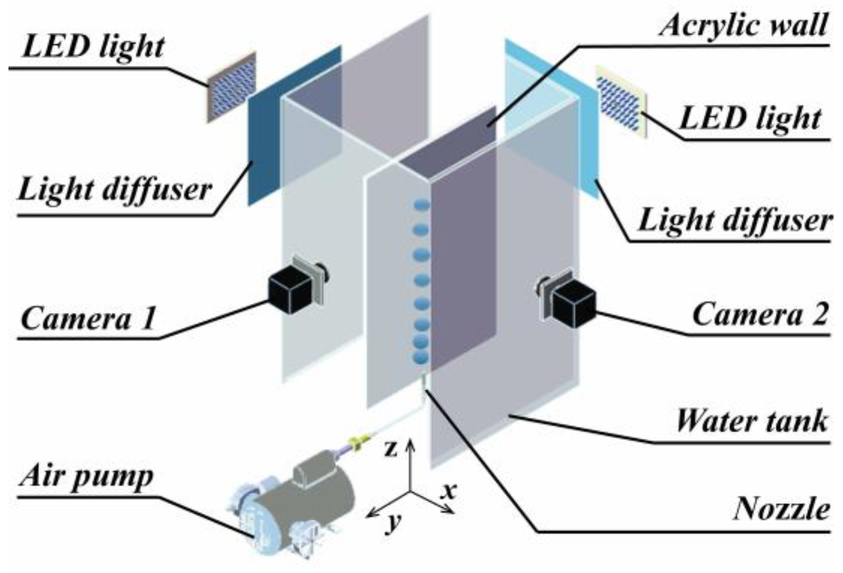
2.1. Experimental Setup

The experimental equipment layout is depicted in Figure 1. The experiment was conducted in a rectangular plexiglass tank measuring 300 mm in length, 300 mm in width, and 650 mm in height. A stainless-steel needle with an outer diameter of 1.48 mm and an inner diameter of 1.12 mm was fixed at the center of the tank’s bottom. The vertical wall was constructed using plexiglass material, with dimensions of 580 mm (length), 200 mm (width), and a thickness of 20 mm. The distance between the wall and the needle was precisely controlled by a lead screw mechanism with an adjustment precision reaching up to 0.1 mm. The z-axis is aligned with the direction of bubble ascent, while the x-axis is perpendicular to the wall, and the y-axis is orthogonal to the xz plane.

The physical parameters of the glycerol aqueous solution are presented in

Table 1. The solution properties at 20 °C.

Liquid Type	Density (kg/m3)	Viscosity (Pa s)	Surface Tension (N/m)
35% glycerin solution	1071.6	6.6 × 10−3	64.14 × 10−3

, considering it as a continuous phase. Additionally, the liquid level within the tank is maintained at 550 mm. A constant pressure flow is provided by the air pump, while the bubble generation frequency is regulated through a micro-regulating valve. The specific bubble generation frequencies employed in the experiment are presented in

Table 2. Frequency of bubble generation.

Frequency	F1	F2	F3
Hz	5	16	38

. The bubble behavior is captured by two orthogonal CCD cameras at a frequency of 180 Hz, with an image resolution of 2048 × 1280 pixels. The test area is illuminated by two LEDs emitting wavelengths of 320–350 nm and 380–420 nm, respectively. Corresponding filters are installed in front of the camera to mitigate interference from ambient light. To achieve homogeneous illumination, sulfuric acid paper is positioned as a light diffuser between the light source and the water tank.

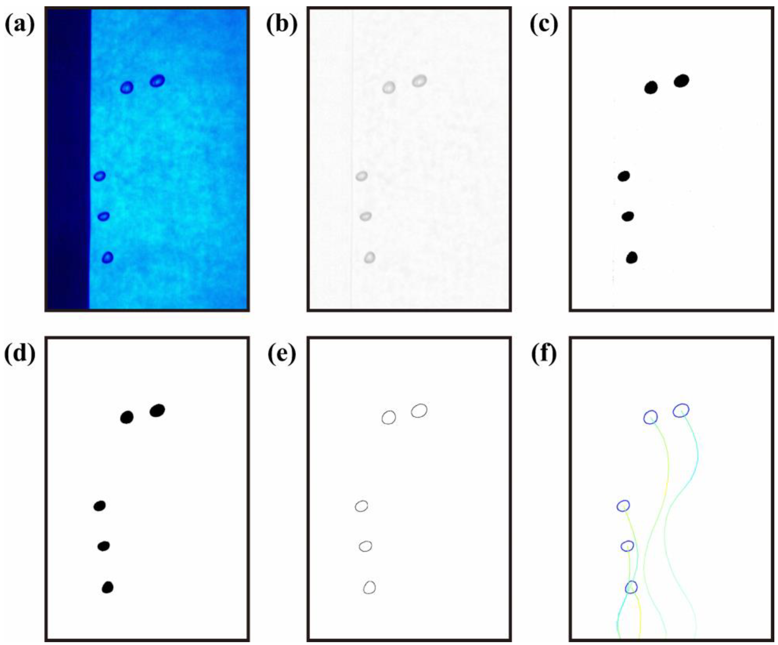
2.2. Bubble Tracking

Bubble tracking is achieved by image processing techniques involving key steps such as image filtering, edge detection, feature extraction and feature matching [17]. The results of these processing steps are illustrated in Figure 2. Initially, a Gaussian low-pass filter is employed to mitigate the noise present in the image signal. The transfer function of this filter can be described as follows [18]:

$$H(m,n)=e^{-\frac{D^2(m,n)}{2{\delta }^2}}$$

(1)

The distance between the coordinate point (m, n) and the center of the spectrum is represented by D(m, n), while δ denotes the standard deviation. The processed image results are illustrated in Figure 2b. The threshold segmentation technique is employed to mitigate the influence of the wall during bubble feature recognition. The transfer function utilized is as follows:

$$g(a,b)=\left\{\begin{array}{l}1,\hspace{1em}\hspace{1em}f(a,b)\ge T\\ 0,\hspace{1em}\hspace{1em}f(a,b)<T\end{array}\right\}$$

(2)

The functions f(a, b) and g(a, b) represent the gray value functions of the original image and the target image, respectively. T denotes a set threshold for gray levels that is utilized to differentiate various regions within an image. The outcome of the process is illustrated in Figure 2c.

The application of threshold segmentation may introduce salt-and-pepper noise and fluctuation interference caused by accidental factors. To mitigate these disturbances, a median filter is employed:

$$h_{ij}=\underset{f_{ij}\in Y}{Med}\left\{f_{ij}\right\}$$

(3)

The gray value of the neighborhood surrounding a point in the original image, denoted as f_ij, is considered within the neighborhood range Y. The middle value obtained from this neighborhood, referred to as Med, is then assigned as the gray value h_ij for that specific point in the output image. The processing results are visually depicted in Figure 2d.

After applying threshold segmentation, the Sobel operator is employed to further delineate the boundaries of the bubbles. For a given image, the gray gradient based on positional coordinates can be represented as:

$$\nabla f=\left[\begin{array}{l}{g}_a\\ g_b\end{array}\right]=\left[\begin{array}{l}\frac{\partial f}{\partial a}\\ \frac{\partial f}{\partial b}\end{array}\right]$$

(4)

The gray-level function f is defined based on the position coordinates in the image. The edge strength is determined by calculating the magnitude of the gray gradient at each point:

$$mag(\nabla f)=\sqrt{{g_a}^2+{g_b}^2}=\sqrt{{\left(\frac{\partial f}{\partial a}\right)}^2+{\left(\frac{\partial f}{\partial b}\right)}^2}$$

(5)

The gradient of each pixel in the target image is computed by taking the difference between the row and column values within a 3 × 3 neighborhood. The center pixel is given a weight of 2 to emphasize its contribution. The resulting calculation can be expressed as:

$$\nabla f=\sqrt{{[(l_7+2l_8+l_9)-(l_1+2l_2+l_3)]}^2+{[(l_7+2l_6+l_9)-(l_1+2l_4+l_7)]}^2}$$

(6)

Here, l_i represents the brightness value of the i-th pixel within the neighborhood. If the gradient value of ▽f at a specific location (a, b) in the image exceeds the threshold, this means that the location is a border pixel, which is an area where the brightness changes more dramatically in the image. The results of the edge detection are presented in Figure 2e.

The feature points in a continuous image frame are matched using a feature matching device, and the corresponding pairs of matched feature points are recorded. The bubble is tracked by evaluating the matching ratio between the selected bubble and the bubble in the subsequent frame, which represents the ratio of successfully matched characteristic points to the total number of characteristic points within the bubble. Once this matching rate exceeds a predefined threshold, the bubble with the highest matching rate is chosen as the tracking object. Figure 2f illustrates the tracking results, where variations in color depict velocity and trajectory is represented by curves on each bubble profile.

The bubble equivalent diameter can be calculated based on the results of bubble edge detection [19]:

$$d_{eq}=\sqrt[3]{{d_h}^2{d}_v}$$

(7)

The long and short axes of the bubble are represented by d_h and d_v, respectively. Figure 3 illustrates the probability density function of bubble sizes corresponding to different generation frequencies. The probability density function of the equivalent diameter of bubbles exhibits an approximate Gaussian distribution. As the frequency of bubble generation increases, there is a slight increment in their diameters, with average equivalent diameters measuring 3.1 mm for frequency F1, 3.2 mm for frequency F2, and 3.8 mm for frequency F3.

Uncertainties in the experimental process arise from the edge-detection process involved in bubble recognition [20]. In cases where the bubble does not collide with the wall, there is a maximum error of ±1 pixel in identifying the bubble’s edges, resulting in an uncertainty of less than 3% in its diameter. However, when a collision occurs between the bubble and the wall, this maximum error increases to ±2 pixels, leading to an uncertainty of less than 5% in its diameter.

3. Results

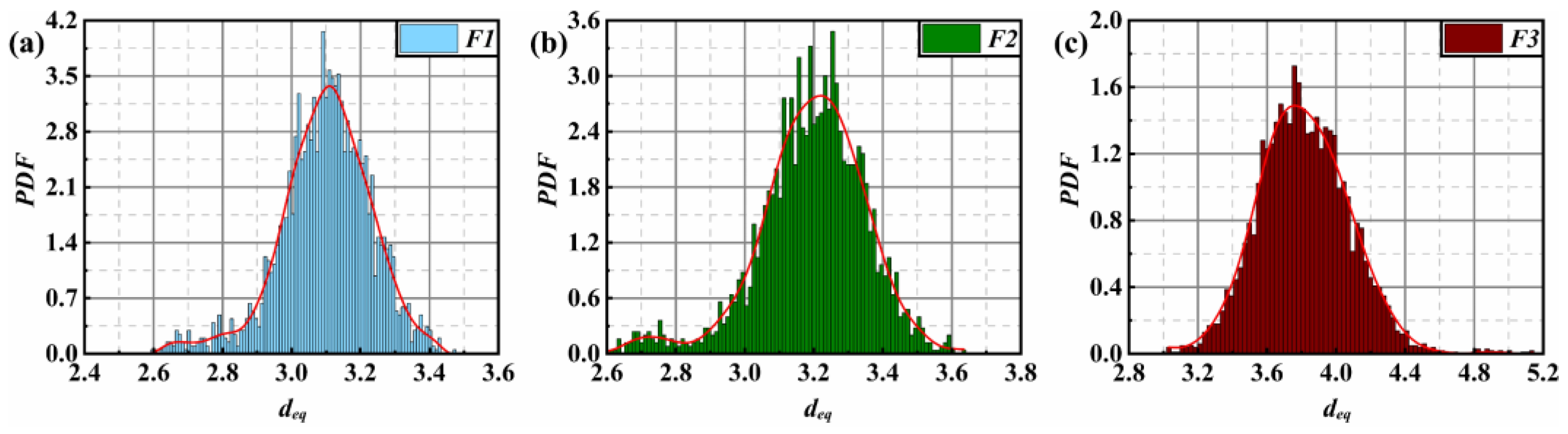
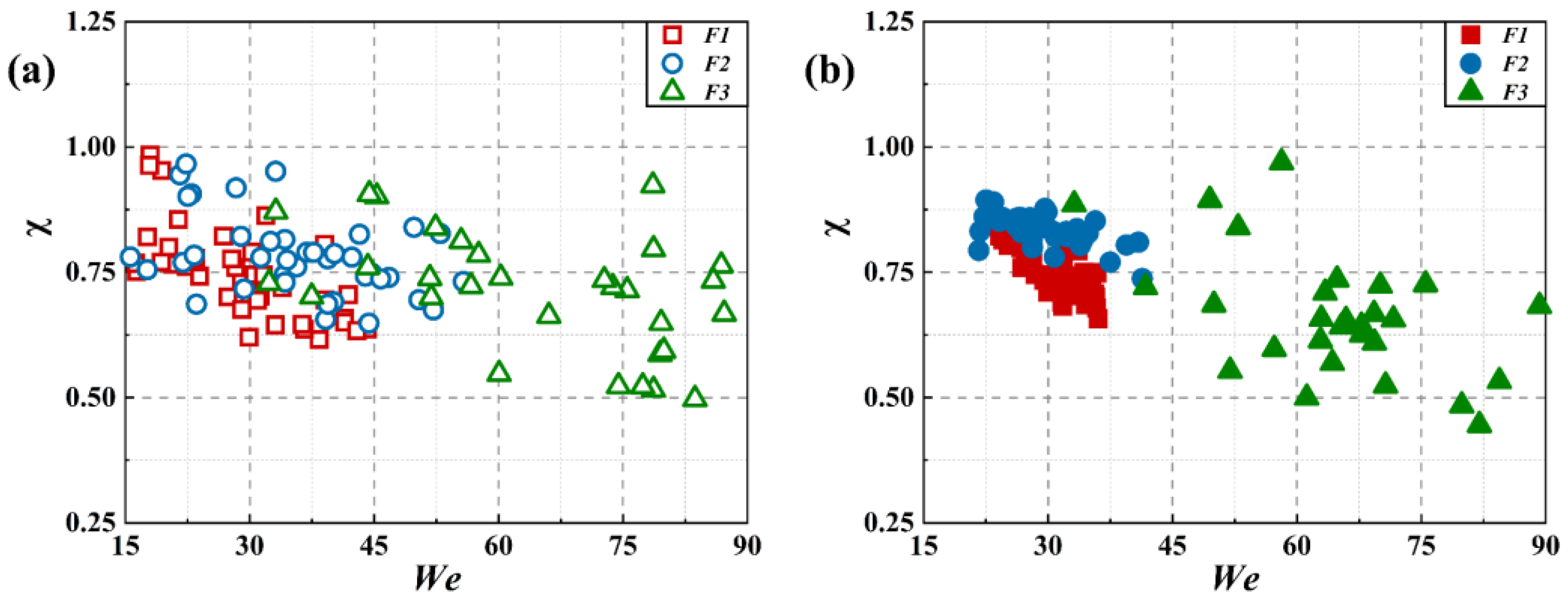
3.1. Statistical Characteristics of Bubble-in-Chain Near the Wall

The influence of wall effects on bubbles can be discerned through the initial wall distance, which denotes the distance from the point of bubble generation to the adjacent wall, i.e., the separation between the bubble-generating needle and the wall [21]. The initial distance is dimensionless, denoted as L* = L/r_eq, where req represents the equivalent radius of the bubble. Its calculation formula can be expressed as r_eq = d_eq/2. In this study, three distinct initial wall distances are chosen (as indicated in

Table 3. Normalized initial wall distance.

Initial Distance	L1	L2	L3
L*	0.5	1.5	3

) to represent strong, medium, and weak wall effects, respectively. Although it is commonly believed that bubble–wall collisions primarily contribute to the reduction of bubble velocity in the near-wall region [1], our findings suggest that, under different operational conditions, other factors besides bubble–wall collisions also influence bubble velocity.

The trajectories of the near-wall bubbles at different generation frequencies are presented in Figure 4. As the bubble generation frequency increases, both the limit velocity and trajectory amplitude of bubbles increase. In the xz plane, there is a more pronounced deviation of bubble trajectories from the wall, whereas in the yz plane, a wider region is covered by bubble trajectories. The bubble velocity is significantly impeded by the wall when the bubble generation frequencies are F1 and F2, respectively. Although the limiting bubble velocity increases as the frequency rises from F1 to F2, it remains low near the wall where the trajectory appears cyan and has a velocity of approximately 0.2 m/s. For the highest frequency, F3, the limiting velocity of bubbles near the wall is larger than that far away from it, indicating that an increase in bubble generation frequency aids in reducing wall-induced velocity inhibition and exerts a positive influence on bubble migration speed.

The effect of the wall on bubble velocity was quantified by averaging the rising velocity and position coordinates of each group of bubbles. The position coordinates and velocity of the bubble were normalized using R_eq and $\overline{V_b}$ (x* = x/r_eq, y* = y/r_eq, V_b* = V_b/$\overline{V_b}$). The relationship between the average velocity and average position is depicted in Figure 5. The wall effect typically induces a reduction in the velocity of individual bubbles [22,23]. The bubble velocity near the wall (x* < 5) decreases as x* decreases when the initial wall distance is L1. The bubble velocity of F1 remains stable at x* = 5. As x* exceeds 8, the velocity of the bubble with frequency F2 gradually decreases, whereas the bubble with frequency F3 starts to decrease at a smaller value of x* and exhibits a more rapid decline. The distribution of bubble velocity changes in a parabolic manner with respect to y*, resembling that observed for free rising bubbles.

When the frequency of bubble generation is fixed, the average velocity of bubbles exhibits a consistent trend at different L*. As x* increases, V_b* gradually rises and stabilizes after reaching a critical value. The x* required to reach the critical velocity decreases with an increase in the L*, while the bubble velocity also exhibits a slight decrease. Particularly at L3, the velocity of the bubble experiences a slight decrease with increasing x* after stabilization. Moreover, V_b* does not exhibit any noticeable regular changes with an increase in y*; however, the velocity distribution is narrower for smaller L*. This phenomenon can be elucidated by the findings of Zeng et al. [14], who demonstrated that near-wall bubbles are influenced by wall-induced lift. In close proximity, the attractive lift generated by the wall effect draws the bubble towards it, thereby restricting its movement within a limited range adjacent to the wall.

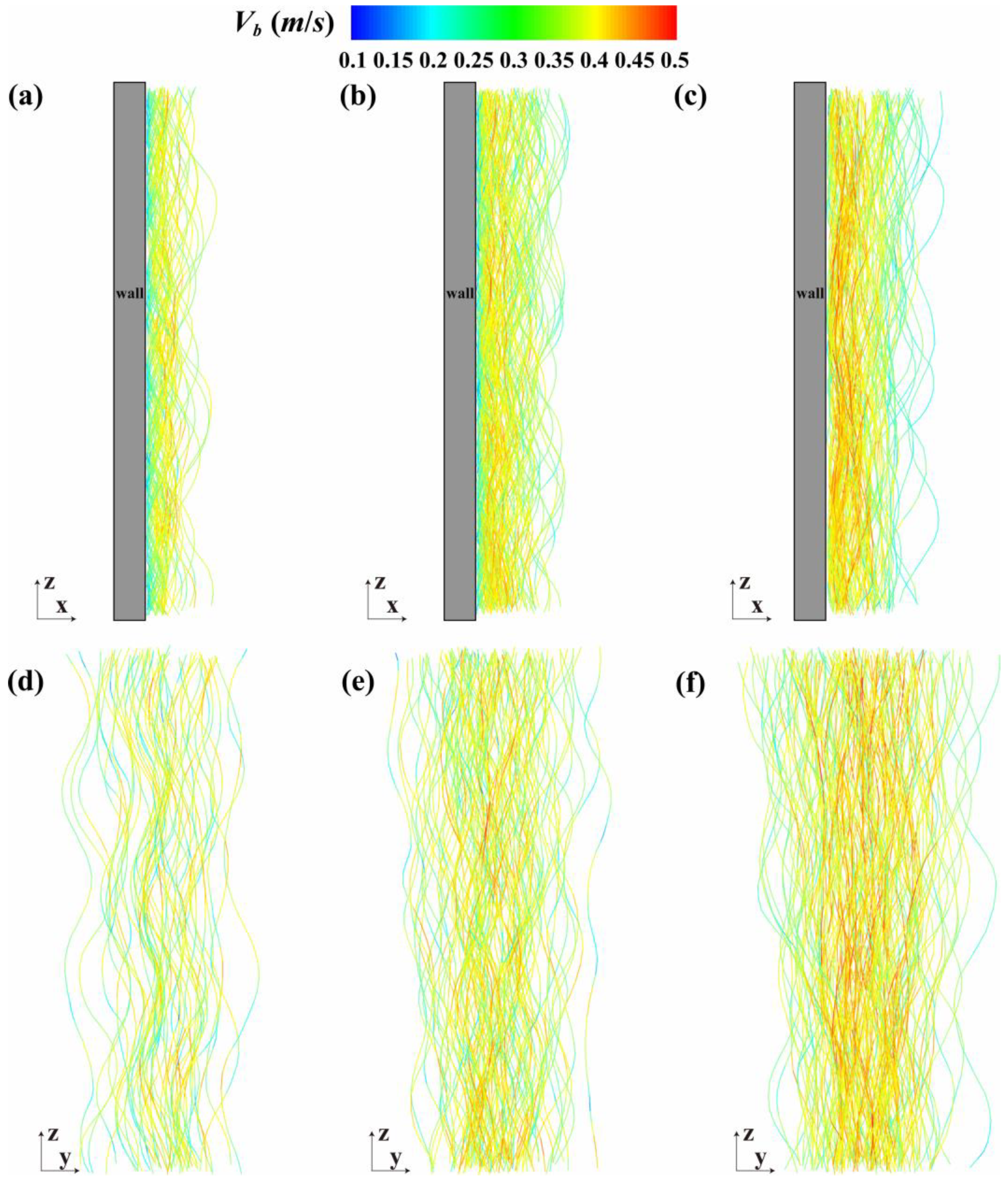
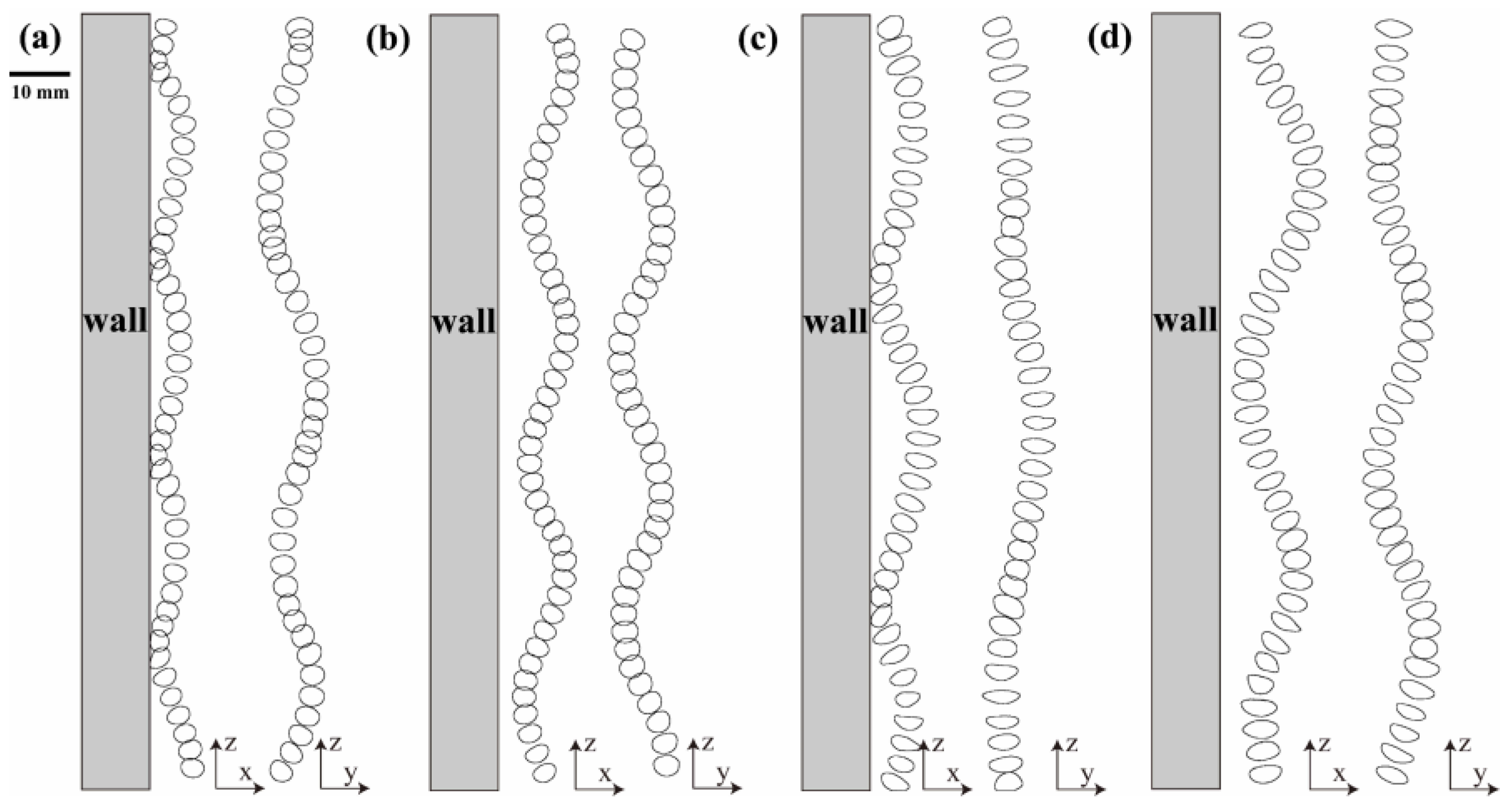
3.2. Motion Mode of the Bubble-in-Chain

The motion of a single bubble near a wall exhibits stochastic behavior and does not consistently adhere to a predetermined migration mode, even under identical operational conditions [24]. The ascent of the bubble-in-chain is influenced by adjacent bubbles, leading to a more intricate migration mode and an increased occurrence of stochasticity within individual bubbles, and it is imperative to analyze their motion modes. The chain of bubbles near the wall exhibits two typical modes of movement: one involves bouncing along the wall, and the other entails forming a spiral upward path near the wall. This differs from the zigzag motion observed in a single bubble during free rising and grants the bubble chain more freedom. The wake induced by the preceding bubble disturbs the bubble-in-chain, causing not only vertical movement towards the wall but also lateral displacement parallel to the wall. This results in a three-dimensional spiral upward trajectory.

The bubble behavior of the two typical modes mentioned above in aqueous glycerol and pure water is depicted in Figure 6. Figure 6a,b illustrate the results in aqueous glycerol solutions, while Figure 6c,d demonstrate the results in pure water. The frequency of bubble generation is F2, and the initial distance from the wall is L1. It is evident that there is a slight increase in bubble size (equivalent diameter from 3.2 mm to 3.6 mm), accompanied by a more significant degree of deformation due to the lower viscosity of pure water. Notably, in glycerol aqueous solutions, a more pronounced bubble–wall collision process occurs with observable close contact between the bubble and the wall, distinguishing it from previous studies on single bubbles [25]. This phenomenon can be attributed to the interaction among adjacent bubbles in the bubble chain and an increase in bubble velocity.

The impact of generation frequency on the bubble rise process is illustrated in Figure 7, particularly when considering the wall effect, where the bubble exhibits a bouncing motion along the wall. The initial distance between the bubble and the wall is set as L1. Figure 7a–c depict the ascending behavior of bubbles under different formation frequencies: F1, F2, and F3, respectively. Upon colliding with the wall, the wavelength of the bubble trajectory increases proportionally to the generation frequency of bubbles, and the frequency of bubble–wall collisions decreases. Even in the absence of collision with the wall, the bubbles maintain a three-dimensional spiral trajectory. During the motion of bubbles, especially during bubble–wall collisions, substantial alteration in shape occurs. These changes can be quantified by considering the aspect ratio (χ = d_v/d_h) and Weber number (We = ρV_b²d_eq/σ).

The relationship between the aspect ratio and Weber number of bubbles at different generation frequencies is depicted in Figure 8. As the Weber number increases, the aspect ratio of the bubble decreases. In the absence of collisions, the distribution of bubble aspect ratios becomes more concentrated with a smaller range of variation, indicating that wall collisions lead to more pronounced shape changes in bubbles. However, it should be noted that even without wall collisions, bubbles formed at high frequencies (e.g., F3) exhibit significant changes in their aspect ratios, suggesting that the high generation frequency itself can induce substantial alterations in bubble shape.

Figure 9 illustrates the variation in the velocity component of bubbles with rising height under different initial wall distances, wherein the velocity and height data have been normalized using the equivalent radius of bubbles and the average velocity (z* = z/r_eq, V_x* = V_x/$\overline{V_b}$, V_y* = V_y/$\overline{V_b}$, V_z* = V_z/$\overline{V_b}$). In the scenario where bubbles collide with the wall, the velocity components along the x-axis and z-axis (V_x and V_z) exhibit periodic variations akin to those observed in a single bubble, with their extremum positions closely aligned. However, the wall-normal velocity component V_y also demonstrates a corresponding relationship; nevertheless, its fluctuations are more pronounced, thereby slightly disrupting its regularity.

When the bubble does not collide with the wall, the velocity component V_z becomes more stable and no longer exhibits obvious periodicity. However, V_x and V_y continue to show periodic variations, but their changing trends are not synchronized and there is a fixed phase difference. It is worth noting that even when there is no collision, V_z displays quasi-periodic oscillations at an initial wall distance of L3. This indicates that the influence of the initial wall distance on bubble motion is complex and can cause changes in velocity components even without collisions.

Figure 10 illustrates the variation of bubble velocity components with height at different generation frequencies. Irrespective of the generation frequency, when bubbles collide with the wall, the velocity components exhibit periodic changes, and the extreme points of different velocity components are closely aligned. However, in cases where bubbles do not collide with the wall, there is no longer consistency in the extreme positions of velocity components and a weakening of V_z’s periodic characteristics can be observed. This suggests that collision processes regulate the periodic features of bubble velocities and synchronize extreme points across different velocity components. As the generation frequency increases, particularly reaching F3, there is a disruption in the periodicity of bubble velocity components to some extent, indicating heightened instability in bubble motion at high frequencies. This instability may arise from complex interactions between bubbles as well as between bubbles and their surroundings, resulting in more intricate and unpredictable variations in velocity components.

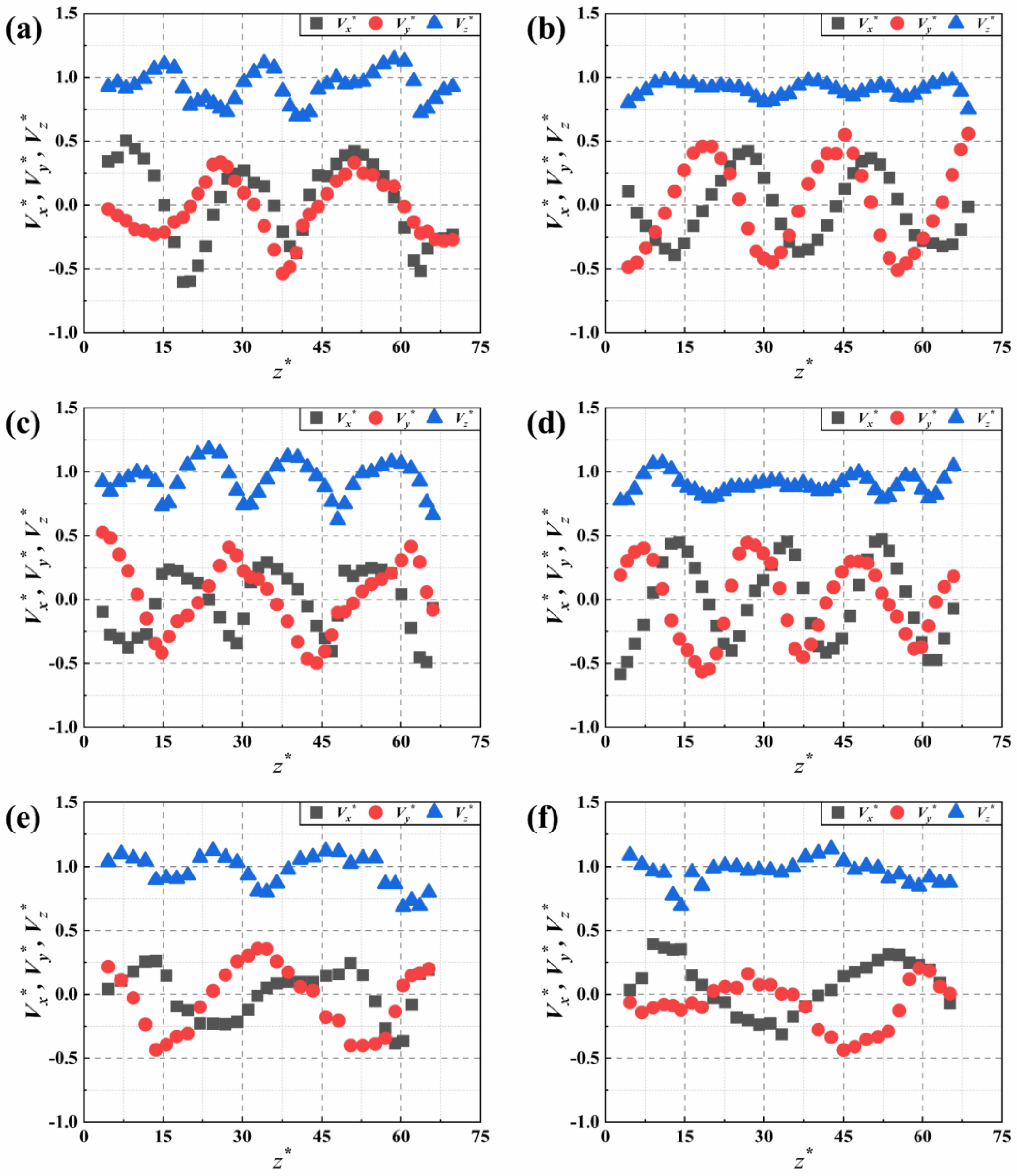
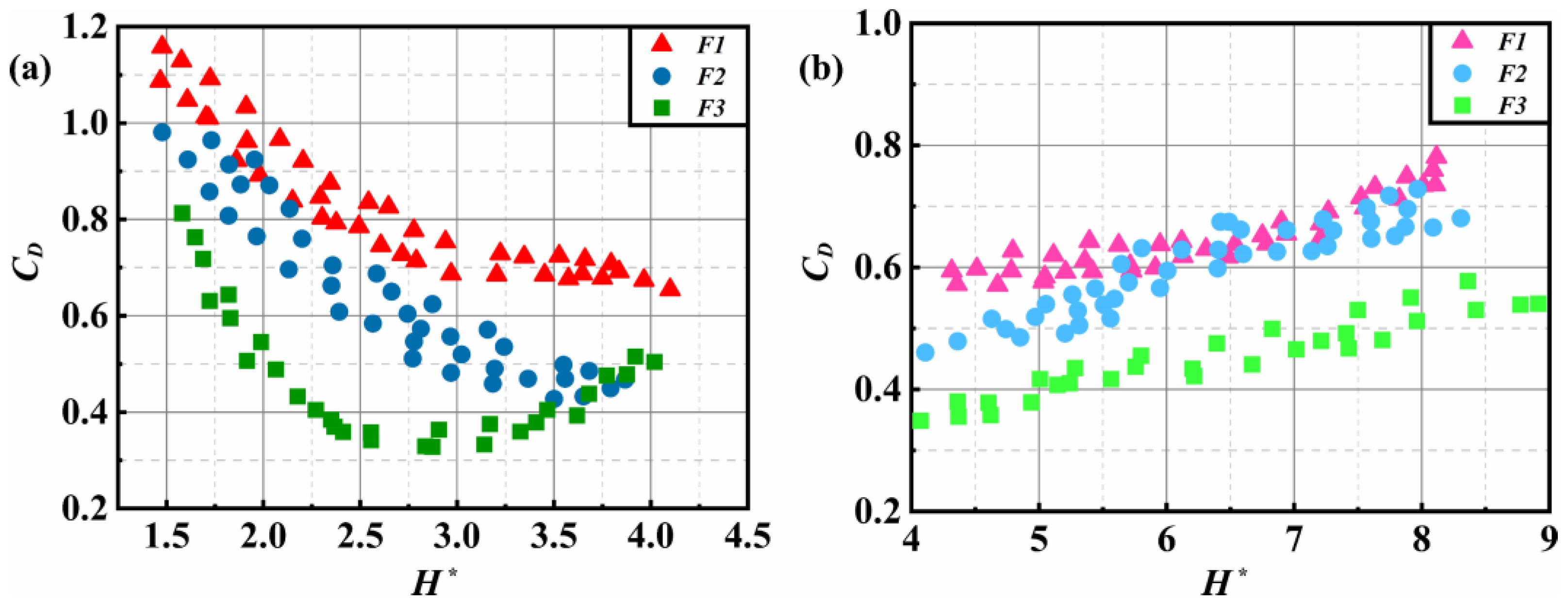
3.3. Dynamic Characteristics of the Bubble-in-Chain

The motion of bubbles is intricately linked to the resistance they encounter. The resistance experienced by a bubble can be determined by the equilibrium between its buoyancy and the resistance [26]:

$$C_D=4\frac{d_{eq}({\rho }_L-{\rho }_G)g}{3{\rho }_L{V_b}^2}$$

(8)

Figure 11 illustrates the correlation between the drag coefficient of bubbles and the Reynolds number at various generation frequencies. The observed trend aligns with previous studies [27,28]. As the Reynolds number increases, the drag coefficient of bubbles decreases across all generation frequencies. Although there is a similarity in the drag coefficient extremum among different generation frequencies, high-frequency bubbles exhibit a wider range of distribution for their drag coefficients. This finding corresponds to the trend observed in average velocity distribution of bubbles, indicating that bubble generation frequency significantly influences their drag characteristics.

The average drag is insufficient to fully capture the influence of the wall on bubbles. The wall effect primarily relies on the distance (H) between the bubble and the wall. By dimensionless treatment of this distance using the equivalent radius of the bubble (H* = H/r_eq), a more precise analysis of the wall effect can be achieved. Figure 12 illustrates, based on motion mode of the bubble-in-chain, the corresponding relationship between bubble drag coefficient and dimensionless distance H*. Irrespective of collision with or without collision against the wall, under all generation frequencies, an increase in H* leads to a decrease in bubble drag coefficient. When the bubble does not collide with the wall, the drag coefficient increases with H*, indicating that wall effects reduce the resistance experienced by the bubble to some extent. Conversely, when the bubble collides with the wall, the drag coefficient decreases with an increase in H*. It is worth noting that for bubbles generated at a frequency of F3, when H* exceeds 3, there is a slight increase in drag coefficient with an increase in H*.

The mechanism of variation in the bubble drag coefficient differs across different modes. The upward flow field induced by the bubble is formed near the wall, which affects the resistance experienced by the bubble. Bubbles that do not collide with the wall move within the main flow area of the induced flow field. As H* increases, the liquid phase velocity decreases and leads to an increase in viscous resistance, resulting in an increase in the resistance coefficient. For bubbles that collide with the wall, when H* is small (less than 2.5), energy conversion and frictional resistance during collision cause an increase in the resistance coefficient. Additionally, a thin liquid film similar to a boundary layer induced by the flow field near the wall experiences rapid decay as H* decreases, leading to a sharp increase in viscous resistance for bubbles and consequently causing an increase in their resistance coefficient [29]. For bubbles generated at the frequency of F3, their strong inducing ability leads to a closer proximity of the mainstream flow field induced by the bubbles to the wall, resulting in an initial decrease followed by an increase in the drag coefficient C_D with increasing H*.

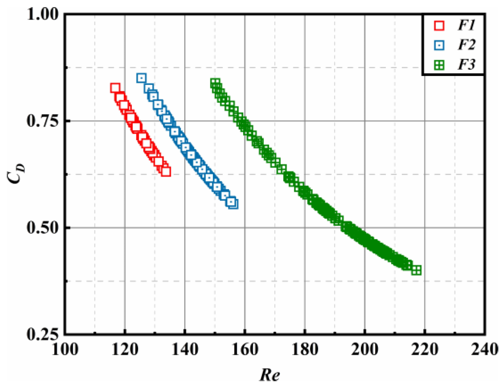
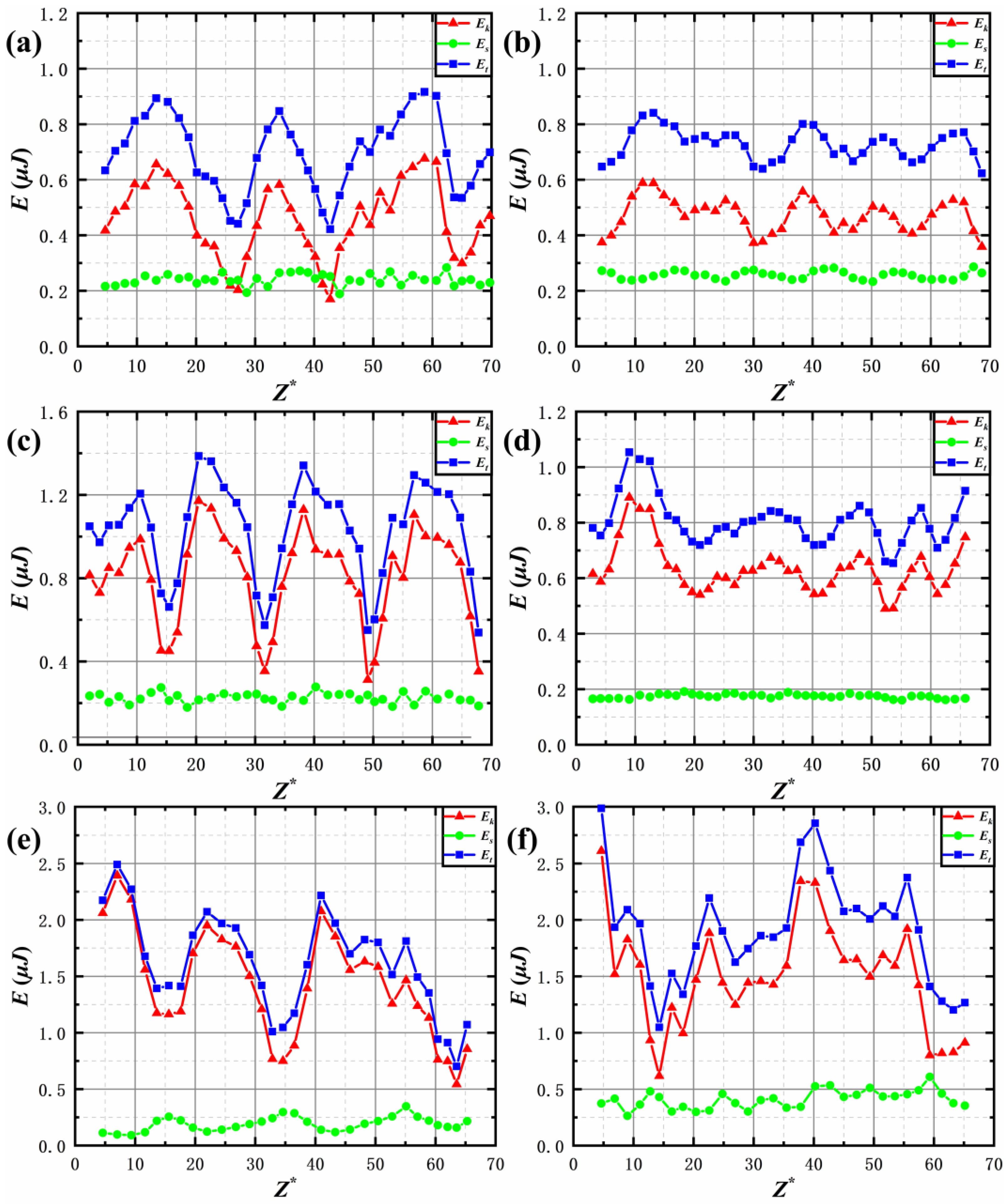
3.4. The Energy Variation of the Bubble-in-Chain

The motion of bubbles near a wall is affected by an additional mass effect of the surrounding fluid, which causes the bubble to carry the surrounding fluid along with it. During this process, the conversion of kinetic energy to surface energy of the bubble plays a crucial role in its dynamic behavior, especially in cases where the wall effect is significant, such as during bubble–wall collisions [27]. To quantitatively describe the kinetic energy and surface energy of the bubble, it can be calculated using the following equations [1]:

$$E_k=\frac{\pi ({\rho }_g+C_m{\rho }_l){d_{eq}}^3{V_b}^2}{12}$$

(9)

$$E_s=\sigma A$$

(10)

$$A=\frac{\pi {d_h}^2}{2}\left(1+\frac{1-e^2}{e}{\tanh }^{-1}e\right)$$

(11)

$$e^2=1-1/{\chi }^2$$

(12)

The coefficient of the additional mass force, denoted as C_m, can be determined by the following equation [29]:

$$C_m=\frac{\alpha }{2-\alpha }$$

(13)

$$\alpha =\frac{2{\chi }^2}{{\chi }^2-1}\left(1-\frac{1}{\sqrt{{\chi }^2-1}}{\cos }^{-1}(1/\chi )\right)$$

(14)

Figure 13 illustrates the dynamic process of energy change in bubbles within pure water and glycerol aqueous solutions. Specifically, Figure 13a,b represent the energy changes of bubbles in pure water, while Figure 13c,d correspond to bubbles in glycerol-water solutions. Figure 13a,c demonstrate the energy change when the bubble collides with the wall, whereas Figure 13b,d depict the energy state when the bubble is not in direct contact with the wall. The gray curve represents the dimensionless path of the bubble, which directly reflects its trajectory under different conditions.

In the case of a bubble–wall collision, the change in energy is closely related to the change in trajectory. The peak of the energy curve aligns with the peak of the bubble’s trajectory. Specifically, in pure water, there is a secondary peak occurring before and after reaching the kinetic energy peak, indicating a significant local increase in kinetic energy before and after colliding with the wall. However, in a glycerol aqueous solution, this secondary peak is significantly inhibited due to increased viscosity, demonstrating a notable impact of viscosity on bubble dynamics. When the bubble does not collide with the wall, its energy changes show a stronger level of randomness. This increased randomness is primarily attributed to the weakening of the wall effect and reduced fluid dynamics constraints on the bubbles. In this case, the surface energy of the bubble remains almost constant in the glycerol aqueous solution when there is no collision with a wall. This indicates that external environmental influences on bubble surface energy need to be exerted through direct contact.

Figure 14 illustrates the impact of bubble generation frequency on changes in bubble energy. Specifically, Figure 14a,c,e depict the energy distribution of bubbles when they collide with the wall, whereas Figure 14b,d,f represent cases where bubbles do not collide with the wall. Figure 14a,b correspond to a bubble formation frequency denoted as F1, Figure 14c,d correspond to a frequency denoted as F2, and Figure 14e,f correspond to a frequency denoted as F3.

The energy composition of a bubble is closely related to its position in the trajectory. Due to the interaction of the wall effect, bubble deformation, and bubble induced flow field, the trajectory of a continuous bubble is more complex and stochastic than that of a single bubble. For a continuous bubble, kinetic energy accounts for the majority of its total energy. As the frequency of bubble formation increases, so does the energy content of each individual bubble. In the process of the collision between the bubble and the wall, the kinetic energy content is at its minimum when the surface energy reaches its maximum value, revealing a remarkable conversion of energy between kinetic and surface energies. At higher generation frequencies, there is a more pronounced peak in bubble surface energy, indicating that higher frequencies enhance both energy storage capacity and the efficiency of bubbles. On one hand, high frequency results in a larger flow rate at the exit during bubble formation, leading to increased bubble energy content; on the other hand, an increase in frequency also enhances the ability of bubble surfaces to deform.

Even if the bubble does not collide with the wall, energy conversion still occurs. However, the trough value of kinetic energy increases, indicating a reduction in kinetic energy loss caused by collision. In contrast, low-frequency bubbles exhibit smaller energy fluctuations. Nevertheless, as the formation frequency increases, so do the energy fluctuations of the bubbles. In some cases, these fluctuations exceed those caused by collision with the wall, suggesting that high-frequency bubbles experience a stabilizing effect from the wall.

4. Conclusions

The experimental investigation focused on studying the motion of near-wall bubble-in-chain with three distinct generation frequencies using a two-camera orthogonal shadow method. Image processing and feature matching techniques were employed to track the motion of the bubble-in-chain. Various motion characteristics such as velocity, size, Reynolds number (Re), and Weber number (We) were determined for these bubbles. Additionally, this study has discussed statistical properties and analyzed motion modes while exploring the dynamic characteristics and energy evolution in detail.

The results demonstrate that both the generation frequency and wall effect significantly influence the behavior of bubbles in a chain. Increasing the generation frequency leads to a more pronounced deviation of bubble trajectories from the wall, resulting in an amplified trajectory amplitude and weakened inhibitory effect of the wall on bubble velocity. It is worth noting that there is a particularly noticeable deviation in xz-plane bubble trajectories and an expanded distribution range for the trajectories in the yz plane. Additionally, with an increase in generation frequency, there is a slight increase in the equivalent diameter of bubbles. The rise in generation frequency intensifies changes in bubble shape and motion instability while partially disrupting periodicity, whereas the wall effect can regulate this periodicity.

The drag coefficients of bubbles with different frequencies consistently decrease as the Reynolds number increases, and higher generation frequencies lead to a wider distribution range for drag coefficients. The wall effect has varying influences on bubbles with different migration modes: for non-colliding bubbles, the drag coefficient increases with greater distance; whereas for colliding bubbles, the drag coefficient decreases as the distance from the wall increases. The conversion of kinetic energy to surface energy during bubble–wall collisions plays a crucial role in determining the motion state. At high generation frequencies, bubbles exhibit more prominent peaks in surface energy, indicating an enhanced capacity for storing and converting energy efficiently.

References

1. Jeong, H.; Park, H. Near-wall rising behaviour of a deformable bubble at high Reynolds number. J. Fluid Mech. 2015, 771, 564–594. [Google Scholar] [CrossRef]
2. Métrailler, D.; Reboux, S.; Lakehal, D. Near-wall turbulence-bubbles interactions in a channel flow at Re τ = 400: A DNS investigation. Nucl. Eng. Des. 2017, 3213, 180–189. [Google Scholar] [CrossRef]
3. Gong, Z.; Cai, J.; Lu, Q. Experiment characterization of the influence of wall wettability and inclination angle on bubble rising process using PIV. Eur. J. Mech./B Fluids 2020, 81, 62–75. [Google Scholar] [CrossRef]
4. Yu, Q.; Ma, X.; Wang, G.; Zhao, J.; Wang, D. Thermodynamic Effect of Single Bubble Near a Rigid Wall. Ultrason. Sonochem. 2020, 71, 105396. [Google Scholar] [CrossRef]
5. Zhang, Y.; Dabiri, S.; Chen, K.; You, Y. An initially spherical bubble rising near a vertical wall. Int. J. Heat Fluid Flow 2020, 85, 108649. [Google Scholar] [CrossRef]
6. Maeng, H.; Park, H. An experimental study on the heat transfer by a single bubble wake rising near a vertical heated wall. Int. J. Heat Mass Transf. 2021, 165, 120590. [Google Scholar] [CrossRef]
7. Yin, J.; Zhang, Y.; Zhu, J.; Lv, L.; Tian, L. An experimental and numerical study on the dynamical behaviors of the rebound cavitation bubble near the solid wall. Int. J. Heat Mass Transf. 2021, 177, 121525. [Google Scholar] [CrossRef]
8. Yuan, J.; Weng, Z.; Shan, Y. Modelling of double bubbles coalescence behavior on different wettability walls using LBM method. Int. J. Therm. Sci. 2021, 168, 107037. [Google Scholar] [CrossRef]
9. Yan, H.J.; Zhang, H.Y.; Zhang, H.M.; Liao, Y.X.; Liu, L. Three-dimensional dynamics of a single bubble rising near a vertical wall:Paths and wakes. Pet. Sci. 2023, 20, 1874–1884. [Google Scholar] [CrossRef]
10. Khodayar, J.; Davoudian, S.H. Surface Wettability Effect on the Rising of a Bubble Attached to a Vertical Wall. Int. J. Multiphas. Flow. 2018, 109, 178–190. [Google Scholar] [CrossRef]
11. Chen, Y.; Tu, C.; Yang, Q.; Wang, Y.; Bao, F. Dynamic behavior of a deformable bubble rising near a vertical wire-mesh in the quiescent water. Exp. Therm. Fluid. Sci. 2021, 120, 110235. [Google Scholar] [CrossRef]
12. Sugiyama, K.; Takemura, F. On the lateral migration of a slightly deformed bubble rising near a vertical plane wall. Fluid Dyn. 2010, 662, 209–231. [Google Scholar] [CrossRef]
13. Sugioka, K.-I.; Tsukada, T. Direct numerical simulations of drag and lift forces acting on a spherical bubble near a plane wall. Int. J. Multiphas. Flow. 2015, 71, 32–37. [Google Scholar] [CrossRef]
14. Zeng, L.; Balachandar, S.; Fischer, P. Wall-induced forces on a rigid sphere at finite Reynolds number. J. Fluid. Mech. 2005, 536, 1–25. [Google Scholar] [CrossRef]
15. Moctezuma, M.F.; Lima-Ochoterena, R.; Zenit, R. Velocity fluctuations resulting from the interaction of a bubble with a vertical wall. Phys. Fluids. 2005, 17, 098106. [Google Scholar] [CrossRef]
16. Zaruba, A.; Lucas, D.; Prasser, H.-M.; Höhne, T. Bubble-wall interactions in a vertical gas–liquid flow: Bouncing. sliding and bubble deformations. Chem. Eng. Sci. 2007, 62, 1591–1605. [Google Scholar] [CrossRef]
17. Gonzales, R.C.; Woods, R.E.; Eddins, S.L. Digital Image Processing Using MATLAB; Pearson Prentice Hall: Hoboken, NJ, USA, 2004. [Google Scholar]
18. Tun, M.T.; Sugiura, Y.; Shimamura, T.J.J.O.S.P. Joint Training of Noisy Image Patch and Impulse Response of Low-Pass Filter in CNN for Image Denoising. J. Signal Process. 2024, 28, 1–17. [Google Scholar] [CrossRef]
19. Li, S.Y.; Xu, Y.; Wang, J.J. Characteristics and Flow Dynamics of Bubble-in-Chain Rising in a Quiescent Fluid. Int. J. Multiphas. Flow. 2021, 143, 103760. [Google Scholar] [CrossRef]
20. Celata, G.P.; D’Annibale, F.; Di Marco, P.; Memoli, G.; Tomiyama, A. Measurements of rising velocity of a small bubble in a stagnant fluid in one- and two-component systems. Exp. Therm. Fluid. Sci. 2007, 31, 609–623. [Google Scholar] [CrossRef]
21. Lee, J.; Park, H. Wake structures behind an oscillating bubble rising close to a vertical wall. Int. J. Multiphas. Flow. 2017, 91, 225–242. [Google Scholar] [CrossRef]
22. Sirino, T.; Mancilla, E.; Morales, R.E.M. Experimental Study on the Behavior of Single Rising Bubbles in a Confined Rectangular Channel. Int. J. Multiphas. Flow. 2019, 145, 103818. [Google Scholar] [CrossRef]
23. Krishna, R.; Urseanu, M.I.; Baten, J.M.V.; Ellenberger, J. Wall effects on the rise of single gas bubbles in liquids. Int. Commun. Heat. Mass. 1999, 26, 781–790. [Google Scholar] [CrossRef]
24. Cai, R.; Ju, E.; Chen, W.; Sun, J. Different modes of bubble migration near a vertical wall in pure water. Korean J. Chem. Eng. 2023, 40, 67–78. [Google Scholar] [CrossRef]
25. Cai, R.; Sun, J.; Chen, W. Near-wall bubble migration and wake structure in viscous liquids. Chem. Eng. Res. Des. 2024, 202, 414–428. [Google Scholar] [CrossRef]
26. Yan, X.; Zheng, K.; Jia, Y.; Miao, Z.; Wang, L.; Cao, Y.; Liu, J. Drag coefficient prediction of a single bubble rising in liquids. Ind. Eng. Chem. Res. 2018, 57, 5385–5393. [Google Scholar] [CrossRef]
27. Clift, R.; Grace, J.R.; Weber, M.E. Bubbles, Drops, and Particles; Dover Publications, Inc.: Mineola, NY, USA, 1978. [Google Scholar]
28. Yan, X.; Jia, Y.; Wang, L.; Cao, Y. Drag coefficient fluctuation prediction of a single bubble rising in water. Chem. Eng. J. 2017, 316, 553–562. [Google Scholar] [CrossRef]
29. Manica, R.; Klaseboer, E.; Chan, D.Y.C. The hydrodynamics of bubble rise and impact with solid surfaces. Adv. Colloid Interface 2016, 235, 214–232. [Google Scholar] [CrossRef]
Figure 1. Experimental setup.
Applsci 14 06076 g001
Figure 2. Bubble tracking processes. (a) original image; (b) low-pass filtering (c) threshold segmentation (d) median filtering (e) edge detection (f) feature matching.
Applsci 14 06076 g002
Figure 3. Probability density function of equivalent bubble diameter with varying bubble generation frequency. (a) have a frequency of F1 and an average equivalent diameter measuring 3.1 mm, (b) have a frequency of F2 and an average equivalent diameter measuring 3.2 mm, and (c) have a frequency of F3 and an average equivalent diameter measuring 3.8 mm.
Applsci 14 06076 g003
Figure 4. The distribution of bubble trajectories with different generation frequencies near the wall: (a,d) have a frequency of F1, (b,e) have a frequency of F2, and (c,f) have a frequency of F3. The initial distance from the wall is L1.
Applsci 14 06076 g004
Figure 5. The average velocity distribution of bubbles. (a,b) consider the effect of different frequencies on bubble velocity, while (c,d) consider the impact of varying initial wall distances.
Applsci 14 06076 g005
Figure 6. Two typical modes of near-wall bubble motion in pure water and glycerol aqueous solution. (a,b) illustrate the results in aqueous glycerol solutions, whereas (c,d) demonstrate the results in pure water. The frequency of bubble generation is F2, and the initial distance from the wall is L1.
Applsci 14 06076 g006
Figure 7. Typical rising mode of bubble-in-chain near the wall at different generation frequencies. The bubble generation frequency of (a) is F1, that of (b) is F2, and that of (c) is F3. The initial wall distance is L1.
Applsci 14 06076 g007
Figure 8. The relationship between the aspect ratio of bubbles with different generation frequencies and the Weber number. (a) The bubbles collide with the wall, (b) The bubbles do not collide with the wall.
Applsci 14 06076 g008
Figure 9. The bubble velocity components at different initial wall distances. (a,c,e) show the cases where bubbles collide with the wall, whereas (b,d,f) show the cases where bubbles do not collide with the wall. (a,b) depict the initial wall distance of L1, (c,d) illustrate the initial wall distance of L2, and (e,f) demonstrate the initial wall distance of L3.
Applsci 14 06076 g009
Figure 10. The variation of bubble velocity components at different generation frequencies. (a,c,e) depict cases where bubbles collide with the wall, whereas (b,d,f) illustrate cases where bubbles do not collide with the wall. The bubble generation frequencies in (a,b) are denoted as F1, those in (c,d) are denoted as F2, and those in (e,f) are denoted as F3.
Applsci 14 06076 g010
Figure 11. The correlation between the average drag of bubbles at different generation frequencies and Reynolds number.
Applsci 14 06076 g011
Figure 12. The bubble drag coefficient varies with H*. (a) Bubble colliding with the wall; (b) bubble not colliding with the wall.
Applsci 14 06076 g012
Figure 13. Energy variations of bubbles in pure water and glycerol aqueous solutions under two typical modes. (a,b) represent energy changes of bubbles in pure water, while (c,d) correspond to bubbles in glycerol-water solutions. (a,c) demonstrates the energy change when a bubble collides with a wall, whereas (b,d) depicts its energy state when it is not in direct contact with a wall. The gray curve represents a dimensionless path of a bubble that directly reflects its trajectory under different conditions.
Applsci 14 06076 g013
Figure 14. Energy variation of bubbles with different generation frequencies. (a,c,e) depict the energy distribution of bubbles upon collision with the wall, whereas (b,d,f) represent the scenario where bubbles do not collide with the wall. (a,b) correspond to bubble generation frequency F1, (c,d) correspond to bubble generation frequency F2, and (e,f) correspond to bubble generation frequency F3.
Applsci 14 06076 g014