Model-Based Design and Testbed for CubeSat Attitude Determination and Control System with Magnetic Actuation

Abstract

This study introduces a robust model-based framework designed for the verification and validation (V&V) of Attitude Determination and Control Systems (ADCSs) in nanosatellites, focusing on magnetic actuation while still being applicable to larger spacecraft platforms. By employing Model-in-the-Loop (MIL), Software-in-the-Loop (SIL), Processor-in-the-Loop (PIL), and Hardware-in-the-Loop (HIL) methodologies, this framework enables a thorough and systematic approach to testing and validation. The framework facilitates the assessment of long-term maneuvers, addressing challenges such as initial small-attitude errors and restricted 3D movements. Two specific maneuvers are evaluated: detumbling and nadir pointing, utilizing quaternions and a comprehensive suite of sensors, including six sun sensors, a three-axis magnetometer, a three-axis gyroscope, GPS, and three magnetorquers. The methodologies—MIL, SIL, PIL, and HIL—integrate the behaviors of digital sensors, analog signals, and astrodynamic perturbations. Based on an optimized SIL environment, Monte Carlo simulations were performed to optimize control gains for nadir pointing, achieving a mean pointing accuracy of 11.69° (MIL) and 18.22° (PIL), and an angular velocity norm of 0.0022 rad/s for detumbling. The HIL environment demonstrated a mean pointing accuracy of 9.96° and an angular velocity norm of 0.0024 rad/s. This comprehensive framework significantly advances the design and verification processes for nanosatellite ADCSs, enhancing the reliability and performance of nanosatellite missions.

1. Introduction

CubeSats, small satellites with diverse applications, are gaining prominence due to their cost-effectiveness and quick development cycles, making them attractive for academic and entrepreneurial aerospace endeavors [1,2,3]. They find utility in Earth observation, environmental monitoring, telecommunications, technology demonstrations, and scientific research [4,5]. CubeSats have been recognized for their role in advancing high-energy astronomy, particularly in gamma-ray sensing, enabling innovative observations and techniques [6].

The reduction in cost associated with CubeSats can be attributed to the standardization of their component subsystems and the availability of low-cost, commercial off-the-shelf (COTS) components. Nevertheless, CubeSats are more prone to failures when subjected to extreme environmental conditions. To mitigate these hazards, international standards such as ISO 19683:2017 [7] and ECSS-E-ST-10-03C [8] have been established. These regulations emphasize rigorous ground testing of CubeSat subsystems to reduce the probability of mission failures [9].

In response to the challenges associated with CubeSat missions, low-cost techniques such as Software-in-the-Loop (SIL), Processor-in-the-Loop (PIL), and Model-in-the-Loop (MIL) have been developed. These methodologies are instrumental in validating the Attitude Determination and Control System (ADCS) algorithms. As emphasized by [10], the reliability of the results obtained from these tests heavily depends on the accuracy of the models used in the simulations. Consequently, many designers [10,11,12] have adopted another advanced technique known as Hardware-in-the-Loop (HIL), which provides more accurate ADCS results by incorporating actual hardware interactions with the simulated environment. For instance, HIL has been employed in real-time configurations to emulate the Earth’s magnetic field using a Helmholtz cage for high-precision calibration [13], as well as for magnetic sensing and actuation tests [14].

Moreover, at various stages of development, models are extensively used for early testing not only in the aerospace industry but also across other industries engaged in R&D. These models serve to eliminate ambiguities and facilitate low-cost test configurations by representing entire systems. Typically, these models are developed in layers, progressing from high-level requirements to detailed technical interactions between components [15]. Especially for low-level configurations, tools such as MIL, SIL, PIL, and HIL significantly reduce development time by enabling extensive testing. In this context, model-based configurations are particularly advantageous for early-stage testing in the development process.

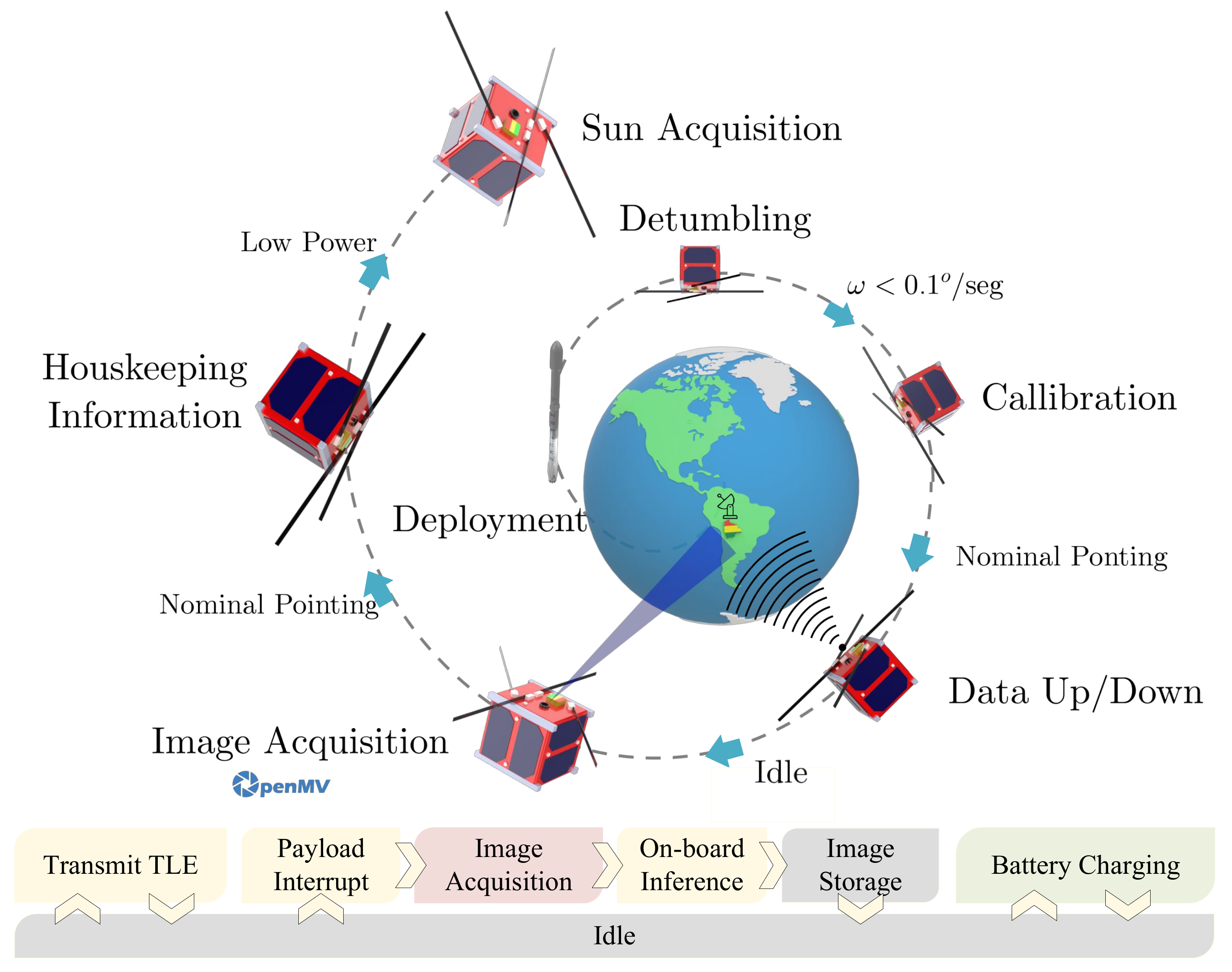
When it comes to subsystems like the ADCS, specific aspects of its performance, physical resources, and operational maneuvers can be meticulously analyzed for all operational modes of a CubeSat. This research aims to establish a robust conceptual design that sets the baseline for CubeSat missions, particularly focusing on Earth observation and on-board image classification, as illustrated in Figure 1. Through the use of mathematical models, it is possible to thoroughly analyze the interaction between a simulated environment and the system via sensors and actuators, such as solar sensors [16] and magnetorquers [17,18]. This approach not only enhances the accuracy and reliability of the ADCS but also contributes to the overall success of CubeSat missions.

Matlab/Simulink is an ideal platform for developing simulated environments due to its extensive range of modules that facilitate the simulation of complex systems. One notable feature is the Simulink Code Generation block, which enables the conversion of simulation models into C code, allowing implementation on embedded devices to replicate the simulated performance [19,20]. However, it is important to note that the ideal simulated performance often differs from the actual performance due to unmodeled disturbances and the non-ideal output of sensors. This discrepancy underscores the need for rigorous validation and calibration to ensure that the simulated environment accurately reflects real-world conditions.

Among other failure factors that may be considered in ground testing are the physical and electronic limitations of the sensors [21]. For the determination of attitude, the sensors must collect reliable values of the variables considered by the control law. Therefore, the attitude control law must be validated to evaluate its robustness to disturbances not modeled in the simulation. Thus, depending on the mission objective and the hardware to be evaluated, it is possible to design a task-specific testbed to optimize the available resources. For instance, in missions requiring a high-precision vector magnetometer, a triaxial fluxgate magnetometer (TFM) is widely used because of its accuracy. However, it requires rigorous calibration. In this scenario, ref. [22] proposes a Magnetically Shielded Room to avoid interference and a Triaxial Uniform Magnetic Field inside to control the vector magnetic field and calibrate the magnetometer. Regarding specific requirements, developers are free to include sun simulators to test sun sensors [23], air bearings to replicate the near-zero gravity environment [9], or custom structures such as floating platforms to simulate spacecraft formation maneuvers using HIL [24].

As previously emphasized, rigorous validation and research processes are crucial to ensure reliable operations under the spatial and electronic constraints of these platforms, especially for developing countries such as Bolivia, to assume the lowest monetary risks in the development process. In this sense, extensive research was carried out in Bolivia to develop a nadir pointing and detumbling controllers for the conceptual design of the country’s first 1U CubeSat, as the main step to improve Bolivia’s building capacity [25]. After the conceptual design of the proposed CubeSat, component-level prototypes were evaluated during stratospheric balloon missions to analyze the robustness and the performance of the simulated controller using real data collected over Amachuma Ground Station (Bolivian Space Agency, La Paz-Bolivia) [26]. These papers underscore the importance of early-stage testing throughout the development process.

In this sense, robust testing protocols also facilitate the integration of a diverse array of payloads on nanosatellites, essential for implementing an ADCS. Such validation is imperative for enabling the deployment of the advanced payloads used in Earth observation, environmental monitoring, space observation, or even communication, which significantly enhance mission success rates [27]. Recent developments are expanding the potential of these nanosatellites; their possible integration with advanced communication modules incorporating 6G networks and quantum technologies [28], or even deep-space exploration tasks for detecting celestial bodies [29], demonstrates their potential and versatility, and underscores the need for robust testing protocols. Given the inherent challenges in CubeSat attitude control compared to larger satellites, achieving precise pointing accuracy is more difficult. This often requires geometric correction methods to improve image quality by correcting distortions present in the captured images. Considering the low-cost test environment provided by stratospheric balloons, a prototype of the payload was developed in 2022 with the mission of classifying images gathered through deep learning [30]. This experiment was considered a first step to validate the on-board computing of complex algorithms for the proposed payload, which in turn is a basis for implementing other imaging components such as high-resolution multispectral cameras to improve the management of terrestrial features and environmental surveillance. This underscores the impact of multispectral imaging technologies in CubeSats, illustrating their role in expanding the scope of data these satellites can capture [31].

Furthermore, these CubeSats, commonly built into 3U to 6U platforms, have been successfully implemented due to their additional space. They have enabled comprehensive monitoring of the atmosphere and oceans, significantly enhancing terrestrial observations [32]. The integration of advanced processing systems allows for high-resolution images to be reconstructed using deep learning techniques, aiding in the identification and monitoring of greenhouse gases and contributing to the assessment of global environmental conditions [33,34,35]. Moreover, these high-resolution images are crucial in detecting natural disasters such as wildfires, utilizing the data provided by these cameras for timely and effective disaster management [36].

While these platforms are typically developed for 3U CubeSats or larger, the applications mentioned above are not limited to larger satellites. For instance, the BIRDS-4 1U CubeSat successfully captured images for monitoring and analyzing landmarks [37]. Wildfire detection has also been developed for a 1U CubeSat, using COTS components to fit power and mass constraints, capturing multispectral images [38]. 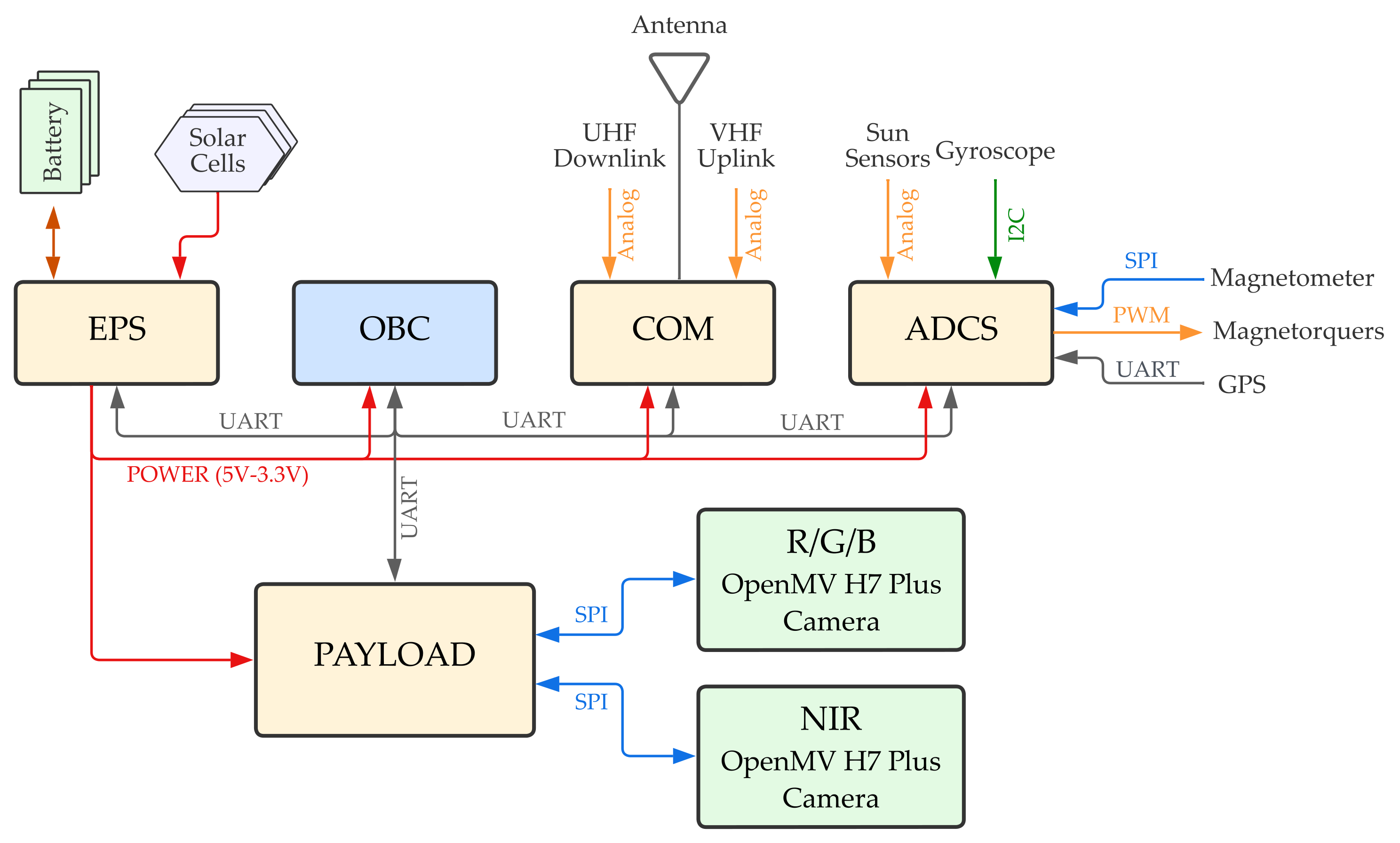Despite their reduced size, these cameras can effectively analyze vegetation and soil moisture [39]. In line with these advancements, a preliminary design of the first Bolivian CubeSat has been developed, as it can be seen in Figure 2. This design includes critical subsystems such as an ADCS, which is currently being tested, as well as EPS, OBC, and COM subsystems. Notably, it features an array of two OpenMV cameras capable of capturing RGB and NIR images, broadening the scope of applications to include the implementations mentioned earlier.

Given the wide variety of available testbeds and considering the technical and economical advantages of using techniques such as SIL, MIL, PIL, and HIL, the purpose of this research is to analyze the different configurations of testbeds mentioned above in terms of models for the proposed controllers. In this way, the performance of both the controller (MIL and SIL) and the embedded system in which the controller is programmed (PIL) will be analyzed, as well as the hardware conditioning and performance in interaction with the simulated environment (HIL). This analysis is an important contribution for nanosatellite developers that, depending on their requirements and verification objectives, can opt for the most optimal decision based on their resources and the specifications that will be shown in each section by configuration, highlighting the feature of simulating attitude maneuvers regardless of initial attitude or restricted movements. Finally, a working scheme based on the V-cycle will also be proposed for the development, validation, and verification process using the proposed framework.

2. ADCS System Model

In this section, the utilized mathematical methods for both attitude estimation and control are described. The model lies in the requirement of computing the imaginary part of the quaternion associated with $\left[BR\right]$ in addition to ${{}^{\mathcal{B}}\mathit{\omega }}_{\mathcal{B}/\mathcal{R}}$, both required for the nadir controller, and ${}^{\mathcal{B}}{\dot{\mathit{B}}}_{\mathrm{Earth}}$ for the detumbling controller.

2.1. Attitude and Orbit Dynamics

The coordinate frames used in this work are Earth Centered Inertial frame (ECI) $\mathcal{N}$: $\{{\widehat{n}}_1,{\widehat{n}}_2,{\widehat{n}}_3\}$, orbit frame $\mathcal{O}$: $\{{\widehat{i}}_r,{\widehat{i}}_{\theta },{\widehat{i}}_h\}$, CubeSat’s body frame $\mathcal{B}$: $\{{\widehat{b}}_1,{\widehat{b}}_2,{\widehat{b}}_3\}$, and reference frame $\mathcal{R}$: $\{{\widehat{r}}_1,{\widehat{r}}_2,{\widehat{r}}_3\}$. The DCM between $\mathcal{O}$ and $\mathcal{R}$ is defined such that $\left[OR\right]=diag\left(\left[\begin{array}{ccc}-1& -1& 1\end{array}\right]\right)$. Notice that this condition ensures that, if $\left[BR\right]={\mathit{I}}_{3\times 3}$, this camera is pointing towards Earth with in addition ${{}^{\mathcal{B}}\mathit{\omega }}_{\mathcal{B}/\mathcal{R}}={\mathbf{0}}_{3\times 1}$. The geometric representation of these reference frames is shown in Figure 3.

Once the nanosatellite operational modes are defined, both rotation and orbit mathematical models are quantified to establish attitude control and estimator methods. In general, an orbit such as that whose eccentricity is zero ($e=0$) is not achievable. In this way, the Gauss variational equations are useful, since these describe the dynamics of the satellite six orbit elements. Let the disturbance orbit force expressed in the orbit frame $\mathit{u}={}^{\mathcal{O}}{\left[\begin{array}{ccc}{u}_r& u_{\theta }& u_h\end{array}\right]}^T$, so the Gauss variational equations are given by the following [40]:

$$\begin{array}{cc}\hfill \dot{a}& =\frac{2a^2}{h}(esin\left(f\right)u_r+\frac{p}{r}{u}_{\theta })\hfill \\ \hfill \dot{e}& =\frac{1}{h}(psin\left(f\right)u_r+((p+r)cos\left(f\right)+re)u_{\theta })\hfill \\ \hfill \dot{i}& =\frac{rcos\left(\theta \right)}{h}{u}_h\hfill \\ \hfill \dot{\mathrm{\Omega }}& =\frac{rsin\left(\theta \right)}{hsin\left(i\right)}{u}_h\hfill \\ \hfill \dot{\omega }& =\frac{1}{he}(-pcos\left(f\right)u_r+(p+r)sin\left(f\right)u_{\theta })-\frac{rsin\left(\theta \right)cos\left(i\right)}{hsin\left(i\right)}{u}_h\hfill \\ \hfill \dot{M}& =n+\frac{b}{ahe}((pcos\left(f\right)-2re)u_r-(p+r)sin\left(f\right)u_{\theta })\hfill \end{array}$$

(1)

Otherwise, the use of these equations is useful when it is intended to develop a formation orbit control algorithm; it also presents a convenient way to analyze the long-term behavior of each orbit element. However, these equations present numerical issues when e is near zero, despite the analytical accuracy of the previous equations; a near-circular orbit is modeled assuming that ${}^{\mathcal{O}}{\mathbf{r}}_{\mathcal{H}/\mathcal{N}}={}^{\mathcal{O}}{\left[\begin{array}{ccc}r& 0& 0\end{array}\right]}^T$ and ${{}^{\mathcal{O}}\mathit{\omega }}_{\mathcal{H}/\mathcal{N}}={}^{\mathcal{O}}{\left[\begin{array}{ccc}0& 0& \sqrt{\frac{{\mu }_{\mathrm{Earth}}}{r^3}}\end{array}\right]}^T$. By applying the transport theorem, it is obtained that ${}^{\mathcal{O}}{\dot{\mathbf{r}}}_{\mathcal{H}/\mathcal{N}}={}^{\mathcal{O}}{\left[\begin{array}{ccc}0& r\sqrt{\frac{{\mu }_{\mathrm{Earth}}}{r^3}}& 0\end{array}\right]}^T$. Furthermore, the rotation matrix $\left[HN\right(t\left)\right]$ can be computed directly from the 3-1-3 rotation given by $\mathrm{\Omega }-i-\theta$; notice that $\theta =\omega +f=\frac{{\mu }_{\mathrm{Earth}}}{r^3}·[t-t\left({\theta }_0\right)]+{\theta }_0$, where f represents the CubeSat’s true anomaly.

Concerning attitude kinematics, it will be modeled using quaternions, which are a compact representation of rotations in 3D space since numerical discontinuities can be avoided. In this work, the quaternion is denoted by $\mathit{q}={\left[\begin{array}{cccc}{q}_1& q_2& q_3& q_4\end{array}\right]}^T={\left[\begin{array}{cc}{\mathit{q}}_v^T& q_4\end{array}\right]}^T=q_1\mathit{i}+q_2\mathit{j}+q_3\mathit{k}+q_4$, so ${\mathit{q}}_v=\left[\begin{array}{ccc}{q}_1& q_2& q_3\end{array}\right]$ represents the imaginary part of the quaternion and $q_4$ the real part. Subsequently, the attitude kinematic differential equation for the CubeSat is given by the following:

$$\begin{array}{cc}\hfill {\dot{\mathit{q}}}_v& =\frac{1}{2}{\mathit{\omega }}_{\mathcal{B}/\mathcal{N}}{q}_4+\frac{1}{2}{\mathit{q}}_v\times {\mathit{\omega }}_{\mathcal{B}/\mathcal{N}}\hfill \\ \hfill {\dot{q}}_4& =-\frac{1}{2}{\mathit{\omega }}_{\mathcal{B}/\mathcal{N}}^T{\mathit{q}}_v\hfill \end{array}$$

(2)

where the DCM matrix associated with $\mathit{q}$ is $\left[BN\right]$. Regarding angular velocity dynamics, the general equations of motion of a satellite equipped with magnetorquers are given by the following:

$$\left[I\right]{\dot{\mathit{\omega }}}_{\mathcal{B}/\mathcal{N}}=-{\mathit{\omega }}_{\mathcal{B}/\mathcal{N}}\times \left[I\right]{\mathit{\omega }}_{\mathcal{B}/\mathcal{N}}+{\mathit{L}}_u+{\mathit{L}}_{\mathit{d}}$$

(3)

where ${\mathit{L}}_u$ is the torque control generated by the magnetorquers. Further, all these vectors and the inertia tensor $\left[I\right]$ are expressed in the body frame $\mathcal{B}$. Assuming the nanosatellite is equipped with three magnetorquers and defining $\left[M\right]=\left[\begin{array}{ccc}{\widehat{\mathit{m}}}_1& {\widehat{\mathit{m}}}_2& {\widehat{\mathit{m}}}_3\end{array}\right]$ where each one represents the unit vector direction for each coil,

$${\mathit{L}}_u=-\left[{\tilde{\mathit{B}}}_{\mathrm{earth}}\right]\left[M\right]\left[\begin{array}{c}{\mu }_1\\ {\mu }_2\\ {\mu }_3\end{array}\right]$$

(4)

where ${\mu }_i$ is the strength of the magnetic dipole torque coil. The magnetorquers proposed for integration within the nanosatellite design are intended to feature a circuit arrangement comprising four layers of internally reconfigurable coils. This design allows for flexible operational configurations, wherein each magnetorquer can be adjusted into parallel, series, or mixed arrays to accommodate specific mission requirements. The resultant magnetic dipole moment of each magnetorquer is described by the following equation:

$${\mu }_i=n_i{A}_i{I}_i$$

(5)

where n stands for the number of turns within a single coil corresponding to each row in the array, A represents the coil’s area on the printed circuit board (PCB), and i denotes the current flowing through the coil. This configuration offers adaptability and current control when establishing the real dipole moment for the satellite’s orientation, thereby facilitating mission success with optimal efficiency. Nonetheless, the disturbance torque can be modeled as follows:

$${\mathit{L}}_d={\mathit{L}}_{GG}+{\mathit{L}}_{aero}+{\mathit{L}}_{mag}$$

(6)

where ${\mathit{L}}_{GG}$ is the gravity gradient torque, ${\mathit{L}}_{aero}$ is the aerodynamic torque, and ${\mathit{L}}_{mag}$ is the magnetic torque. All aforementioned disturbance torques are expressed in the body frame $\mathcal{B}$. Notice that, in LEO, the effect of the solar pressure is at least one order of magnitude smaller than the other phenomena, while the aerodynamic drag increases. In addition, to introduce a representative disturbance of disturbance torque, its maximum value is approximated in the next sections, and the resulting torque is introduced into the model as a Gaussian random vector with a sample time of $T_s$, such that $\mathit{L}\{d-\max \}\sim \mathcal{N}(\mathbf{0},{\sigma }_{\omega }^2{\mathit{I}}_{3\times 3})$; the standard deviation ${\sigma }_{\omega }=T_s{L}_{d-max}{I}_{min}^{-1}$ where $I_{min}$ is the minimum value of the diagonal of the inertia tensor [25]. Notice that an analytical value for ${\mathit{L}}_{GG}$, $\mathit{L}aero$, and ${\mathit{L}}_{mag}$ could be approximated for each one; however, this goes beyond the scope of this work.

Gravity Gradient Torque. The interaction of the forces of gravity and the CubeSat body is different in each part of the body, so a gravity gradient is produced as an effect of this difference along the body, around its center of mass. Otherwise, the maximum Earth gravity gradient could be approximated as follows:

$$L_{GG}=\frac{3G{M}_{\oplus }}{2R_C^3}|I_z-I_y|\sin \left(2\theta \right)$$

(7)

where $I_z$ and $I_y$ are the moments of inertia about the z- and y-axis correspondingly (shown in

Table 1. Astrophysical parameters.

Name	Abbreviation	Value
Universal gravitational constant	G	$6.67408\times {10}^{-11}$ m3 kg−1 s−2
Mass of the Earth	$M_{\oplus }$	$5.972\times {10}^{24}$ kg
Orbit		Altitude: 400 km, inclination: ${30}^{\circ }$
Orbit radius	$R_C$	6770 km
Atmospheric density	$\rho$	$3.725\times {10}^{-12}$ kg/m3
Drag coefficient	$C_D$	$\approx 2.2$
Velocity	V	$\sqrt{\frac{G{M}_{\oplus }}{R_C}}=7669.3$ m/s
Incident satellite surface area	$A_{inc}$	0.01 m2
Local magnetic field—Bolivia	$\parallel {\mathit{B}}_{\mathrm{Earth}-\mathrm{local}}\parallel$	[18,528.2, −3447.5, −4780.5] nT
Residual dipole	D	0.01 Am2
Distance between $CoM$ and $Cpa$	$|r_{aero}|$	0.05 m

), and $\theta$ is the maximum deviation of the orbit frame Z-axis. A convenient approximation can be made considering the worst-case scenario where $\sin \left(2\theta \right)=1$ with the constants shown in Table 1.

Aerodynamic Torque.- Due to the atmospheric density, there is an atmospheric drag that especially affects LEO spacecraft and decreases exponentially as altitude increases. Therefore, the aerodynamic force produced by drag is shown in the following equation:

$$F_{aero}=\frac{1}{2}\rho C_D{A}_{inc}{V}^2$$

(8)

where $\rho$ is the atmospheric density at a given altitude, V is the nanosatellite velocity, $C_D$ is the drag coefficient, and $A_{inc}$ is the incident satellite surface area. Hence, the aerodynamic force calculated is $2.410\times {10}^{-6}$ N and the maximum aerodynamic torque can be calculated by (9), where $r_{aero}$ is the vector from the center of pressure ($Cpa$) to the center of mass ($CoM$) of the CubeSat (${\mathit{r}}_{aero}={\mathit{r}}_{Cpa}-{\mathit{r}}_{CoM}$). For practical purposes related to maximum disturbance analysis, we assume that $\parallel {\mathit{r}}_{aero}\parallel =0.05\left[m\right]$.

$$L_{aero}=F_{aero}\parallel {\mathit{r}}_{aero}\parallel$$

(9)

Magnetic Torque.- The interaction between a magnetic dipole and a magnetic field produces a torque, which can be modeled as follows:

$${\mathit{L}}_{mag}=\mathit{m}\times \mathit{B}$$

(10)

where ${\mathit{L}}_{mag}$ stands for the magnetic torque vector, $\mathit{m}$ the magnetic dipole moment vector, and $\mathit{B}$ the magnetic field vector. Taking into account the WMM2020, the Earth’s magnetic field expressed in the NED frame (North–East–Down) can be modeled as follows:

$${{}^{NED}\mathit{B}}_{earth}(\lambda ,\varphi ,r,t)=-\nabla V(\lambda ,\varphi ,r,t)$$

(11)

such that

$$\nabla V(\lambda ,\varphi ,r,t)=a\sum _{n=1}^N{\left(\frac{a}{r}\right)}^{n+1}\sum _{m=0}^n[g_n^m\left(t\right)cos\left(m\lambda \right)+h_n^{m}sin\left(m\lambda \right)]P_n^m(sin\varphi )$$

with $\lambda$ longitude, $\varphi$ latitude, r radius, $N=12$, $a=6371.2$ [Km] geomagnetic reference radius, and t time. Additionally, the maximum disturbance magnetic torque produced by the own nanosatellite structure can be approximated as follows:

$$L_{mag}=D\left|{\mathit{B}}_{Earth-reference}\right|$$

(12)

where D is the nanosatellite residual dipole in Am². Finally, all the maximum disturbance values are shown in

Table 2. Maximum disturbance torque.

Perturbation	Abbreviation	Value [Nm]
Gravity gradient torque	$L_{GG}$	$1.347\times {10}^{-10}$
Aerodynamic torque	$L_{aero}$	$1.205\times {10}^{-7}$
Magnetic torque	$L_{mag}$	$1.944\times {10}^{-7}$
Total torque	$L_{d-max}$	$3.150\times {10}^{-7}$

.

2.2. Attitude Determination Algorithm

Before computing the attitude controller, an attitude determination method is needed for both sunlight and eclipse zones. Regardless of the zone, an Extended Kalman Filter (EKF) is applied in order to estimate the state vector $\mathit{x}={\left[\begin{array}{cc}{\mathit{\omega }}^T& {\mathit{q}}^T\end{array}\right]}^T$. Due to the hardware restrictions of the selected MCU, the aforementioned WMM2020-2025 is used, noting that the change of frame between NED and $\mathcal{O}$ is given by the following:

$${{}^{\mathcal{O}}\mathit{B}}_{\mathrm{Earth}}=\left[\begin{array}{ccc}-sin\left(\varphi \right)·cos\left(\lambda \right)& -sin\left(\varphi \right)·sin\left(\lambda \right)& cos\left(\varphi \right)\\ -sin\left(\lambda \right)& cos\left(\lambda \right)& 0\\ -cos\left(\varphi \right)·cos\left(\lambda \right)& -cos\left(\varphi \right)·sin\left(\lambda \right)& -sin\left(\varphi \right)\end{array}\right]{{}^{NED}\mathit{B}}_{\mathrm{Earth}}$$

(13)

Furthermore, assuming a sunlight zone, the Triad method is applied to get the DCM $\left[BN\right]$ as follows. First, the Triad vectors are computed:

$${{}^{\mathcal{B}}\widehat{\mathit{t}}}_1={}^{\mathcal{B}}\widehat{\mathit{s}},{{}^{\mathcal{B}}\widehat{\mathit{t}}}_2=\frac{{}^{\mathcal{B}}\widehat{\mathit{s}}\times {}^{\mathcal{B}}\widehat{\mathit{v}}}{\parallel {}^{\mathcal{B}}\widehat{\mathit{s}}\times {}^{\mathcal{B}}\widehat{\mathit{v}}\parallel },{{}^{\mathcal{B}}\widehat{\mathit{t}}}_3={{}^{\mathcal{B}}\widehat{\mathit{t}}}_1\times {{}^{\mathcal{B}}\widehat{\mathit{t}}}_2$$

(14)

And

$${{}^{\mathcal{N}}\widehat{\mathit{t}}}_1={}^{\mathcal{N}}\widehat{\mathit{s}},{{}^{\mathcal{N}}\widehat{\mathit{t}}}_2=\frac{{}^{\mathcal{N}}\widehat{\mathit{s}}\times {}^{\mathcal{N}}\widehat{\mathit{v}}}{\parallel {}^{\mathcal{N}}\widehat{\mathit{s}}\times {}^{\mathcal{N}}\widehat{\mathit{v}}\parallel },{{}^{\mathcal{N}}\widehat{\mathit{t}}}_3={{}^{\mathcal{N}}\widehat{\mathit{t}}}_1\times {{}^{\mathcal{N}}\widehat{\mathit{t}}}_2$$

(15)

where $\widehat{\mathit{s}}$ is the sun direction computed by using the gathered measurement for the six sun sensors and $\widehat{\mathit{v}}$ is the magnetic field vector. Then, the DCM description $\left[BN\right]$ is given by the following:

$$\left[BT\right]=\left[\begin{array}{c}{{}^B\widehat{\mathit{t}}}_1{{}^B\widehat{\mathit{t}}}_2{{}^B\widehat{\mathit{t}}}_3\end{array}\right]$$

(16)

$$\left[NT\right]=\left[\begin{array}{c}{{}^N\widehat{\mathit{t}}}_1{{}^N\widehat{\mathit{t}}}_2{{}^N\widehat{\mathit{t}}}_3\end{array}\right]$$

(17)

$$\left[BN\right]=\left[BT\right]{\left[NT\right]}^T$$

(18)

So, the quaternion $\mathit{q}$ corresponding to $\left[BN\right]$ is computed using Shepperd’s method [41], which avoids division by zero. Additionally, the continuous computation of $\mathit{q}$ from $\left[BN\right]$ may lead to numerical discontinuities in $\mathit{q}$, caused by switching to $-\mathit{q}$, which represents the same rotation as $\mathit{q}$. Consequently, a mechanism is needed to ensure the numerical continuity of the quaternion. Assuming an adequate sampling time for the ADCS such that a sign switch occurs between $q_{{\max }_{K+1}}$ and $q_{{\max }_K}$, and considering that a quaternion satisfies $|q_{\max }|\ge 0.5$, it follows that $|q_{{\max }_{K+1}}-q_{{\max }_K}|=|-q_{{\max }_{K+1}}-q_{{\max }_K}|=2|q_{{\max }_{K+1}}|\ge 1$. Thus, $|q_{{\max }_{K+1}}-q_{{\max }_K}|\ge 1$ is used to check for quaternion sign switching. Additionally, the Shepperd method first computes the largest value $q_{\max }^2$ from $\{q_1^2,q_2^2,q_3^2,q_4^2\}$. By applying the aforementioned criteria to $q_{\max }$ and $-q_{\max }$, quaternion numerical discontinuity is avoided.

Moreover, as it was mentioned earlier, the DCM $\left[HN\right]$ can be quantified assuming a circular orbit. However, to predict this matrix it can be computed through the Triad method:

$${\widehat{\mathit{i}}}_r=\frac{\mathit{r}}{\left|\mathit{r}\right|},{\widehat{\mathit{i}}}_{\theta }={\widehat{\mathit{i}}}_h\times {\widehat{\mathit{i}}}_r,{\widehat{\mathit{i}}}_h=\frac{\mathit{r}\times \dot{\mathit{r}}}{|\mathit{r}\times \dot{\mathit{r}}|}$$

(19)

$$\left[HN\right]=\left[\begin{array}{ccc}{\mathit{i}}_r& {\mathit{i}}_{\theta }& {\mathit{i}}_h\end{array}\right]$$

(20)

where $\mathit{r}$ is estimated by an orbit propagator or GNSS receiver; for this work, just the orbit propagator case is considered. Otherwise, for applying the EKF, the dynamics should be expressed as follows:

$$\begin{array}{cc}\hfill \dot{\mathit{x}}& =f_d(\mathit{x},{\mathit{L}}_u)+\mathit{w}\hfill \end{array}$$

(21)

$$\begin{array}{cc}\hfill \mathit{y}& =h_d(\mathit{x},{\mathit{L}}_u)+\mathit{v}\hfill \end{array}$$

(22)

where $\mathit{w}$ and $\mathit{v}$ are disturbances. Next, the required equations for EKF are presented:

$$\left[\begin{array}{c}\dot{\mathit{q}}\\ \dot{\mathit{\omega }}\end{array}\right]=\left[\begin{array}{c}\frac{1}{2}\mathbf{\Omega }\left(\mathit{\omega }\right)\mathit{q}\\ {\left[I\right]}^{-1}(-\left[\tilde{\mathit{\omega }}\right]\left[I\right]\mathit{\omega }+{\mathit{L}}_u)\end{array}\right]+\left[\begin{array}{c}\mathbf{0}\\ {\mathit{\omega }}_{\mathrm{drift}}+\mathcal{N}(0,{\left(I_{min}^{-1}{L}_{d-max}\right)}^2)·{\mathbf{1}}_{3\times 1}\end{array}\right]$$

(23)

Notice that the discrete EKF will be implemented. By discretizing this system, it will also introduce a discretization error, which in turn will introduce process noise to ${\mathit{q}}_k$ and ${\mathit{\omega }}_k$.

2.3. Attitude Control Algorithm

Detumbling.- To maintain safety conditions and reach good initial conditions to apply the nadir controller, detumbling control is applied to try to achieve these requirements. For this purpose, the B-dot control is applied:

$${}^{\mathcal{B}}\mathit{m}=-C{{}^{\mathcal{B}}\dot{\mathit{B}}}_{\mathrm{Earth}},C>0$$

(24)

Nadir control.- In order to reach $\left[BR\right]\to {\mathit{I}}_{3\times 3}$, the following control law is proposed for nadir control:

$${}^{\mathcal{B}}\mathit{m}=-\frac{1}{\parallel {\mathit{B}}_{\mathrm{Earth}}\parallel }{{}^{\mathcal{B}}\mathit{B}}_{\mathrm{Earth}}\times (K_P{\mathit{q}}_v+K_D{}^{\mathcal{B}}{\mathit{\omega }}_{\mathcal{B}/\mathcal{R}}),K_P>0,K_D>0$$

(25)

where the DCM matrix associated with ${\mathit{q}}_v$ is $\left[BR\right]$. The purpose of nadir control is to make the magnetic dipole go to zero. For this to be achieved, the states of the system, which are the quaternions and the angular rates, need to reach zero. This means that the body frame ($\mathcal{B}$) is perfectly aligned with the reference frame ($\mathcal{R}$). Notice that, if it is assumed that ${\mathit{B}}_{\mathrm{Earth}}$ is periodic, then the proposed control guarantees ${\mathit{q}}_v\to \mathbf{0}$ with the next four asymptotically stable local equilibrium points $\{{\widehat{r}}_1=\pm {\widehat{i}}_r,{\widehat{r}}_3=\pm {\widehat{i}}_h\}$ [42].

3. Simulation Environment and Approaches

3.1. Model in the Loop

Extending the ideal simulation environment developed in [25], the Model-in-the-Loop (MIL) environment depicted in Figure 4 integrates comprehensive attitude and orbit dynamics. This setup incorporates the World Magnetic Model (WMM) 2020–2025, the DE405 solar system model, and a conic eclipse model to predict sunlit, umbra, and penumbra conditions [43]. The MIL environment employs various sensors: the MMC5603NJ magnetic field sensor (16-bit resolution per axis), the SLCD-61N8 Coarse Sun Sensor (12-bit resolution, restricted by the STM32F411RE MCU), and the L3GD20 gyroscope (16-bit resolution per axis). These sensors are subjected to white noise, bias, misalignments, nonorthogonalities, quantization, and a sampling time of 0.01 s.

Sensor signals are simulated and packed into a 32-byte vector. This data packet is then transmitted to the attitude estimator, where it is unpacked, and the attitude estimation algorithm is applied. The controller computes the required three-axis magnetic moment (12 bits per axis, constrained by the MCU’s PWM resolution), which is then packed and sent back to the simulated space environment. This framework is crucial for the systematic integration of subsequent simulation approaches and allows for flexible integration with various communication protocols. The following subsections delve into the developed simulation models for both sun sensors and magnetorquers, considering the constraint of achieving real-time execution.

3.1.1. Sun Sensor Model

The Simulink implementation of the solar sensor model for the control system is based on the addition of six SLCD-61N8 photodiodes. These sensors were modeled for implementation in the verification framework. The objective was to simulate an environment, accounting for the response of electronic components of interest, such as those receiving external signals. Implementing the electronic circuits with the solar sensors included allows for a simulated environment with additional considerations, such as noise and typical errors in the signals obtained, which are later processed by the next control stages.

These photodiodes simulate current signals in a controlled manner, which are given by the equation $I=R·A·\beta$ where R is the incident solar irradiance in the area, A is the active area, and $\beta$ is the chosen sensitivity of the photodiode. The electronic conditioning circuit was designed to convert the input signal provided by the photodiode (given by the output current I) into an output voltage signal V sun sensor proportional to the aforementioned input. The model chosen for the design was based on the topology of the instrumentation amplifier circuit [44]. This was carried out to condition the signal to a voltage output. In addition, a low-pass filter [45] was added for output stability, high-frequency signal filtering, and electrical isolation for each photodiode. To obtain a voltage output relative to a current input, the traditional instrumentation amplifier topology was adapted to one containing two trans-impedance amplifiers and a differential amplifier (Figure 5). This arrangement allows for a linear relationship between the circuit voltage output and the photodiode input current. The gain is mainly determined by the feedback resistor ratio and the resistors $R_4$ and $R_3$ as follows:

$$V_{out}=2·R_F·\left(\frac{R_4}{R_3}\right)·I_{in}$$

(26)

The circuit design aspects for achieving the correct gain in the impedance circuit were analyzed based on the maximum short-circuit current of the SLCD-61N8 photodiode. The typical current for this photodiode is 170 $\mathsf{\mu }$A at an irradiance of 25 mW/cm². Therefore, for a total solar irradiance of 136.7 mW/cm², a maximum current of 929 $\mathsf{\mu }$[A] is obtained through linear ratio calculation.

The values assigned to $R_F$, $R_3$, and $R_4$ in the Simulink model are $390\left[\mathrm{\Omega }\right]$, 2.7 k$\left[\mathrm{\Omega }\right]$, and 12 k$\left[\mathrm{\Omega }\right]$, respectively. It is important to note that both resistors $R_3$ and $R_4$ must match $R_1$ and $R_2$ to ensure a correct output voltage of approximately 3.25 [V], with a maximum current flow of 929 $\mathsf{\mu }$A. The signal from each sun sensor is processed by the previously explained circuit, and the circuit’s output reveals the output voltage of the sun sensor model. Additionally, the implementation block of one of the six sun sensors is depicted in Figure 5.

3.1.2. Magnetorquer Model

The implementation of the magnetorquer models in Simulink aimed to enhance simulation reliability by incorporating the various components that influence the system of these actuators. The control system circuit for this setup is depicted in Figure 6. Additionally, the objective was to examine whether the effects of loading and unloading the coils significantly impact the controller’s performance. The design of the magnetorquer system included selecting components and setting values to simulate common errors that occur during the operation of integrated circuits.

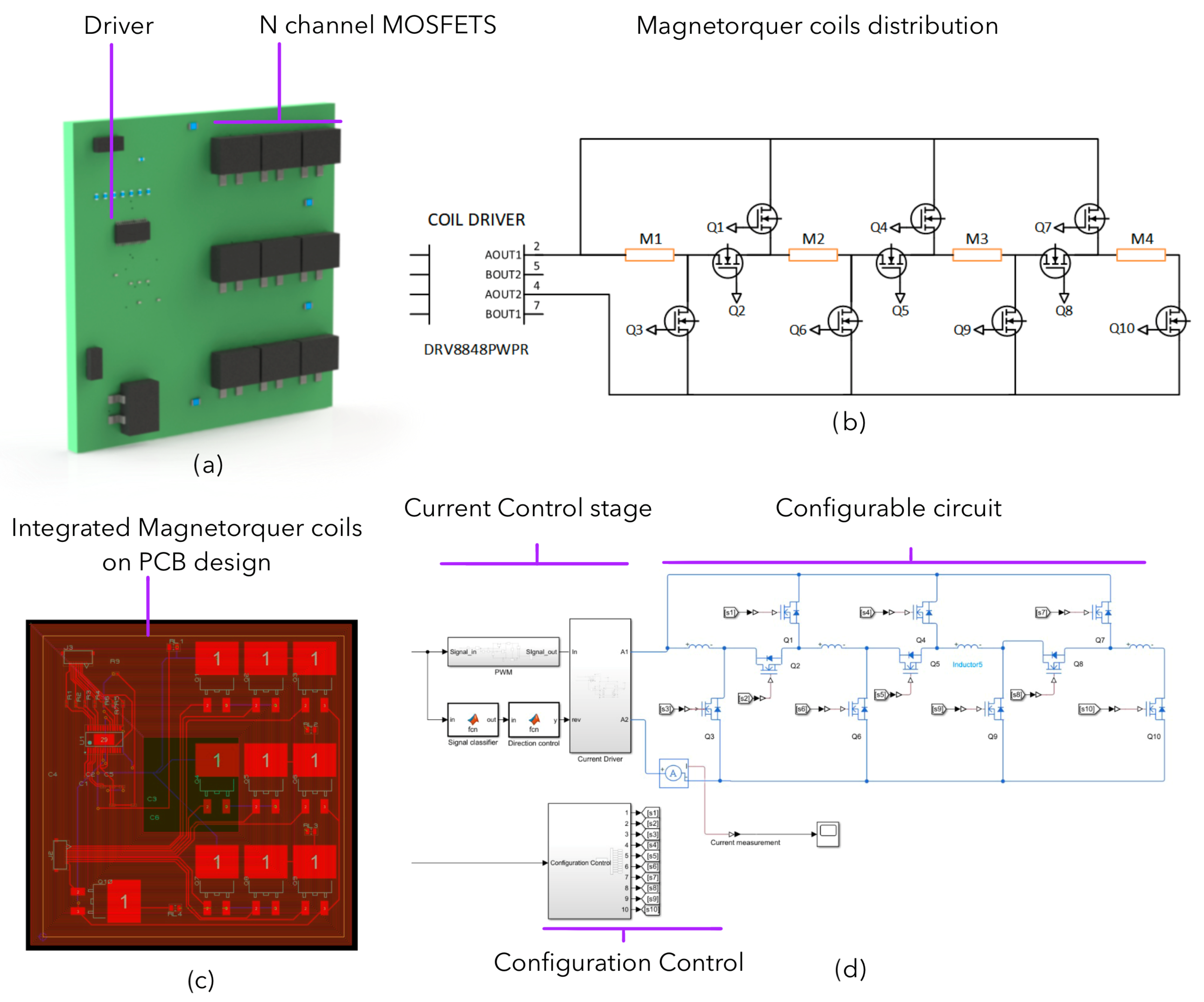
Each magnetorquer is depicted in a diagram with a set of four coils, configurable using MOSFETs, as shown in Figure 6b. This flexibility allows each magnetorquer to be arranged in parallel, series, or mixed arrays. Moreover, the ICDRV8848 motor controller [46] is considered for precise current flow control [47].

To meet the dipole moment requirements determined by the tested control system, values are processed using known and established data on the number of turns and the area of each magnetorquer, as expressed in Equation (5). This calculation determines the necessary current flow through each set of coils. These calculated values are then transmitted to the controller ports to ensure an adequate current supply to the magnetorquers. Depending on the current demands, the configuration control system adjusts the arrangement of the four coils by varying the activation and deactivation of ten MOSFETs, visible in Figure 6d, that act as switches. Representative models were chosen for each coil to closely approximate real component behaviors, incorporating resistance and capacitance [48] into each coil model. This comprehensive approach ensures that the simulations closely mimic real-world scenarios, thereby enhancing the accuracy and reliability of the magnetorquer system’s performance evaluation.

For each coil in any magnetorquer configuration, the magnetic moment is given by a term $D_{or}$, so the relationship between voltage and current must be adjusted so that each coil receives the same current. The voltage and current supplied by the controller are characterized by the following equivalences:

$$V=n·V_o,I=m·I_o$$

(27)

Likewise, the total magnetic moment generated by each magnetorquer is given by the following:

$$D_{total}=(n·m)·D_o$$

(28)

where n and m are the number of rows and columns of coils for the established configuration.

This process was integrated into the magnetorquer control system in Simulink with its general behavior previously explained. For a more detailed simulation, physical aspects such as the number of turns of 60 and a resistance of $70\left[\mathrm{\Omega }\right]$ are considered within the modeling of each of the three magnetorquer systems. The other parameters adopted are shown in

Table 3. Single magnetorquer parameters.

Parameter	Value
Number of turns	60
Trace width	0.3 mm
Thickness	20 $\mathsf{\mu }$m
Space between traces	0.1 mm
Magnetorquer resistance	70 $\mathrm{\Omega }$
Outer length	80 mm
Inner length	26 mm

, determined thanks to [49]. The current through each coil is 0.020 A, the maximum current allowed being 0.80 A in the configuration of the four coils in parallel.

The schematic design of this magnetorquer control circuit was performed at PROTEUS, where the assembly for the PCB was carried out. Figure 6a shows a CAD model of the PCB for this model. In Figure 6c, the circuit layout can be seen, as well as the magnetorquer coils integrated on the PCB.

In the model visible in Figure 6d, the circuit designed in Simulink can be observed, where the data processing based on the calculated current is performed. Through a PWM signal with a current direction indicator, a simulated block mimics the driver behavior with outputs coupled to the reconfigurable magnetorquer coil circuit. The control configuration block is responsible for making series or parallel reconfigurations as needed. The creation of these models was made possible through the use of Simscape Electrical components. This is because the Simscape Electrical models integrate directly with Simulink main block diagrams and an analysis of their physical behavior is possible using PS converters. The model configuration for the operation of the sensor models based on the previously developed electronic circuits is the fixed step and ode1be (Backward Euler) solver. The fundamental sampling time in the configuration must be small enough for the correct simulation of the PWM signal that affects the circuit during the driver controller stage; however, this parameter was modified for the other simulations.

3.2. Software in the Loop

To ensure the correct functioning and overall performance of the ADCS, both for controller debugging and characterization of its performance under several scenarios, SIL simulations were executed and evaluated using the Monte Carlo analysis to evaluate the controller’s efficiency. Moreover, the development of the SIL environment was built upon the MIL environment. Since it is intended that the implementation of the control algorithm be executed through real-time simulation in Simulink, interfaced with an STM32 microcontroller, and taking into account that sensor readings are performed directly by the controller, the Embedded Coder application within Simulink was used to generate and optimize C code for each subsystem.

The code generation workflow required aligning the sample times of the simulations with that of the controller to ensure single-rate code generation (avoiding timing functions that are only available for CPUs). The controller processed signals from the plant model and computed control signals within the defined sample interval. The solver configuration was set to fixed step, using the Real-Time ODE1b for environments that includes SimScape models and RK4 for the remaining. The system’s target file was configured to ert.tlc, and the programming language was set to C99 (ISO) in the Code Generation section in the model setting configuration parameters, which is widely supported by most embedded systems. It is crucial to confirm that both Simulink and STM32 Cube IDE are configured to use the ISO C99 standard [50]. To ensure this configuration in Simulink, the process involved accessing “Model Settings”, selecting “Code Generation”, and choosing “C99 (ISO)” under “Language Standard”. Activating C99 in STM32 Cube IDE required navigating through “File”, then “Properties”, selecting “C/C++ Build”, accessing “Settings”, and choosing “Toolchain Settings”, with “GNU99 (ISO C99+gnu extensions)(-std=gnu99)” selected under “Language Standard”. For effective code generation, parameters must be handled as atomic units and the model should be converted to a referenced model. This conversion allows the specification of variables and ensures that the behavior of the referenced model remains consistent, regardless of its position in the model hierarchy. Before initiating code generation, it is essential to establish specific naming rules for auto-generated identifiers, tailored to each subsystem. This necessity arises from the requirement to generate multiple codes within the same Simulink model. In our scenario, three codes were generated: nadir controller, detumbling controllers, and a filter for the magnetometer measurements. Consequently, the name of the file in the “Code for component” section was modified accordingly. Upon configuring these settings, the Embedded Coder app could be used to generate the code and build the model. The generated library files were stored in a designated folder, named in the penultimate step of the process. To deploy the C code on the C-caller function (Simulink function for executing .c and .h files) or hardware, the library files were included in the Simulink workspace and also copied into the Inc directory of the STM project. Within the main project file, it was necessary to invoke the model_initialize function and the model_step function to facilitate proper integration and execution of the SIL simulation or hardware deployment. In this way, the ADCS model developed in MIL was deployed in C code, allowing for an optimized code of the entire system. Furthermore, once the model was converted into C code and executed by SIL, it strongly suggested embedding compatibility into an STM32 Nucleo board for further testbed trials to validate the attitude controller.

Moreover, to optimize SIL time consumption, and computational demands and to address computational overheads, all of the remaining model functions were turned into subsystems which could then be turned into Matlab S functions. This transformation from subsystem to S function implies a conversion of the block into C code with its corresponding .mex file, where the mex file links all the C functions to distinct Simulink operations. Consequently, the model was greatly optimized for a streamlined approach within a local CPU allowing for a less demanding simulation and SIL testbed testing.

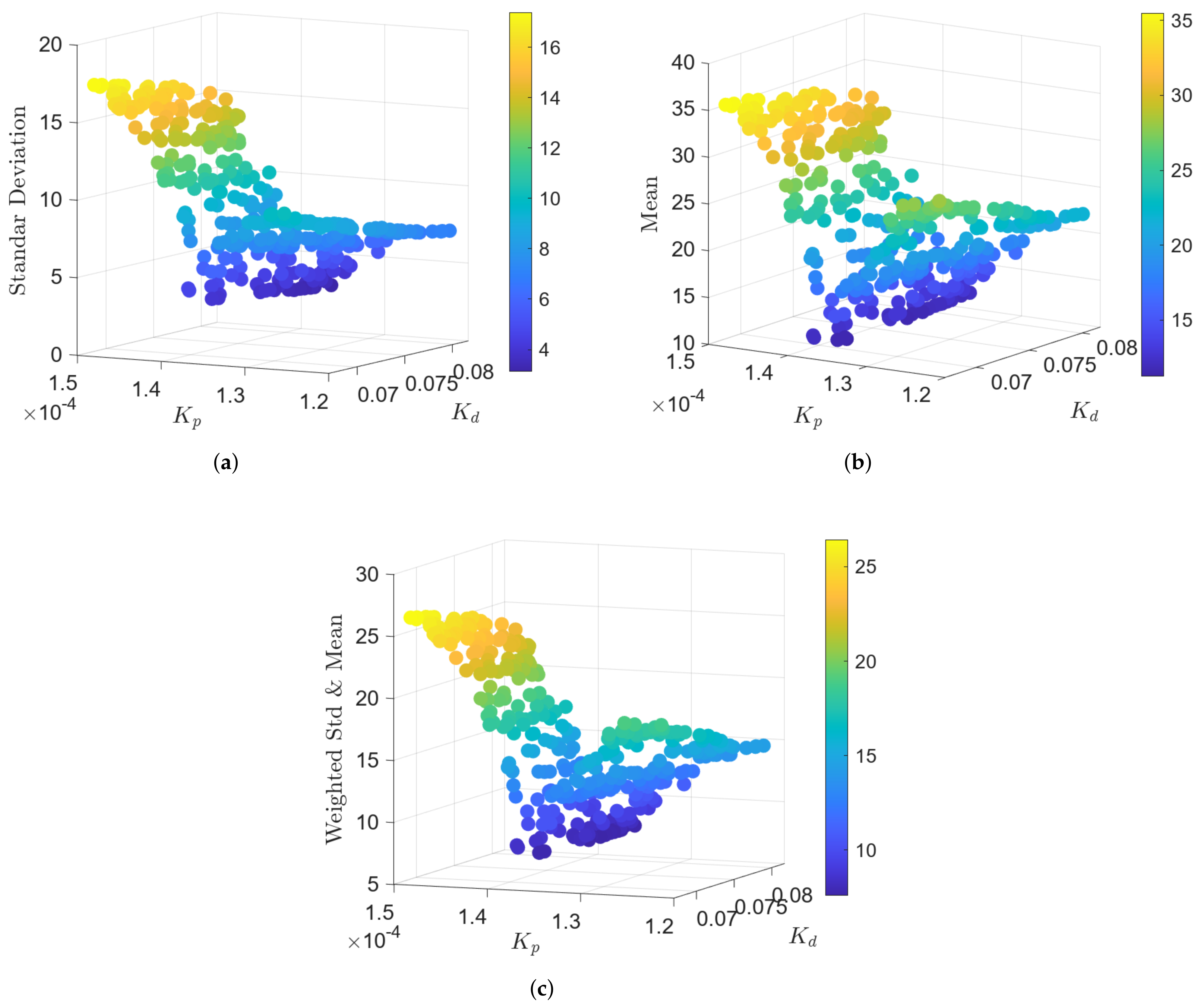
Once the S functions were implemented in the Simulink simulation environment, Monte Carlo simulation was carried out, and sensitivity analysis was used to iterate with random values evaluating the variability of the pointing error under different external perturbations and initial conditions. Sensitivity analysis requires the use of global variables to facilitate variations in the initial parameters, which requires the implementation of inputs to Simulink blocks that use those parameters.

As initial parameters, an analysis of $K_p$ and $K_d$ was carried out through 350 iterations of random values using a normal distribution. Consequently, $(K_p=0.00013555)$ and $(K_d=0.0743)$ were determined as optimal gains for the ADCS. Using these gains, an analysis of variations in the initial orbit, inertia matrix, Euler angles, orbit elements, and angular velocity was implemented. For the initial orbit condition, Euler angles, inertia matrix, and angular velocity, the generation of random values was through a uniform distribution using custom requirements to obtain the results of the Monte Carlo simulation. The said custom requirements in sensitivity analysis determined the standard deviation and mean of the pointing error starting from a 10,000 s mark to avoid initial noise measurements.

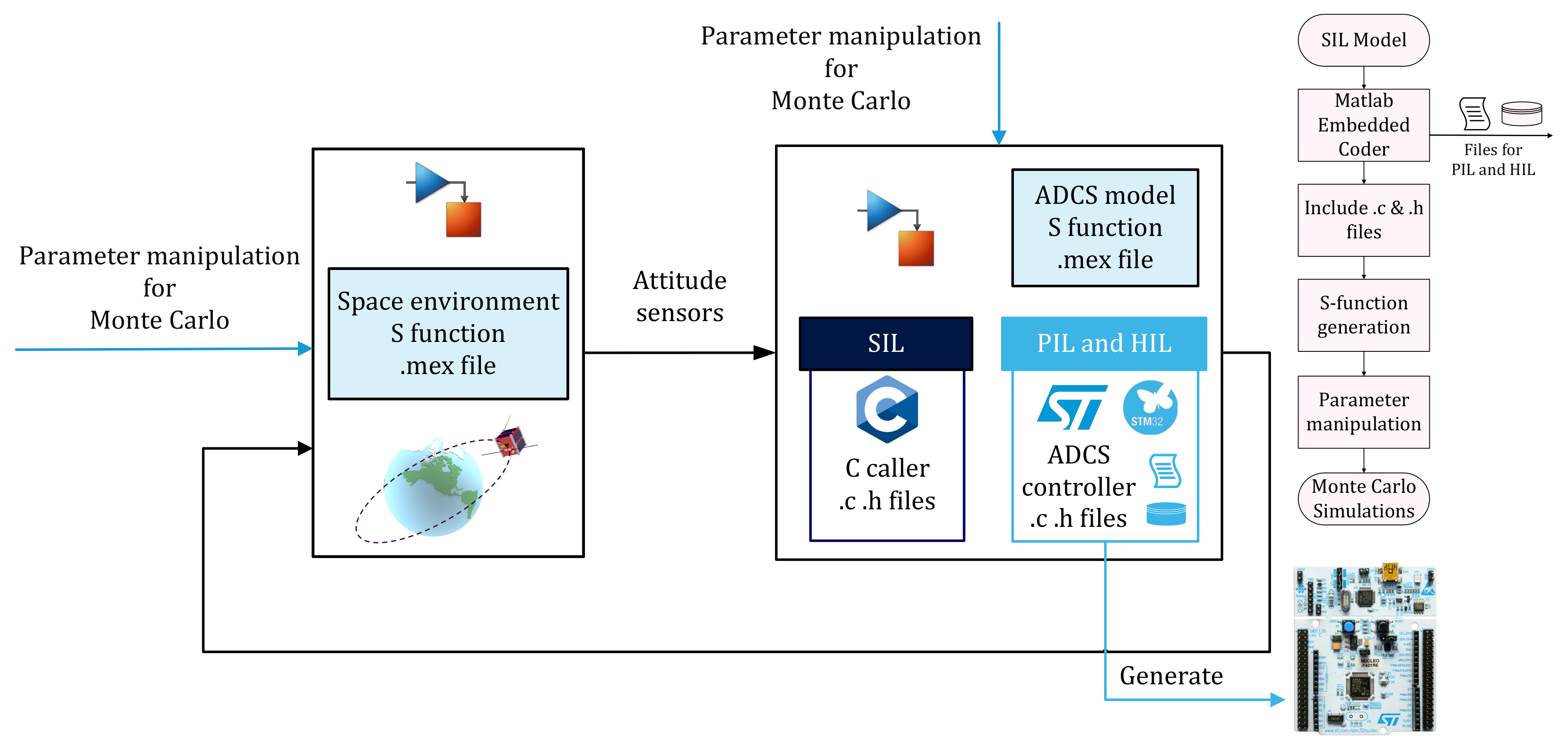
Finally, to derive a proper model for SIL testbed evaluation, a Simulink model was constructed using the optimized S-function performance, C caller embedded code, and optimal Monte Carlo gains. Figure 7 shows the overall SIL framework and methodology for testbed evaluation and data derived towards PIL and HIL evaluations.

3.3. Software and Hardware Configuration for PIL and HIL

3.3.1. Characteristics of the PIL and HIL Environment

Processor-in-the-Loop (PIL) simulations are employed to incorporate sensor simulation feedback and emulate the space environment, enabling the verification of ADCS behavior as though operating in space. The PIL method establishes a foundational framework for the pilot phase of the system including the target processor. In our configuration, Matlab in the host computer connects to the STM32 via a serial connection. During a representative Simulink simulation, the plant model transmits data to the controller in the form of a 32-byte vector, with each element being an 8-bit integer. Upon receiving the data, the controller processes the information for one sample interval by executing its C-generated code, and then sends the output back to the Simulink real-time simulation, completing one sample cycle. Additionally, the HIL real-time simulations incorporate specific hardware components to increase the fidelity of the simulation. In particular, a Helmholtz cage is utilized to derive magnetic field values, simulating the geomagnetic field experienced by the CubeSat in its body frame $\mathcal{B}$ during its orbital motion. The difference between the PIL and HIL approaches lies in the real magnetometer measurement for HIL. Nevertheless, PIL employs the magnetometer data simulated by the space environment. Finally, it is emphasized that both PIL and HIL consider the space environment developed for MIL. So, the Simscape model developed for sun sensors and magnetorquers is simulated during the real-time tests.

3.3.2. Sensor Emulator

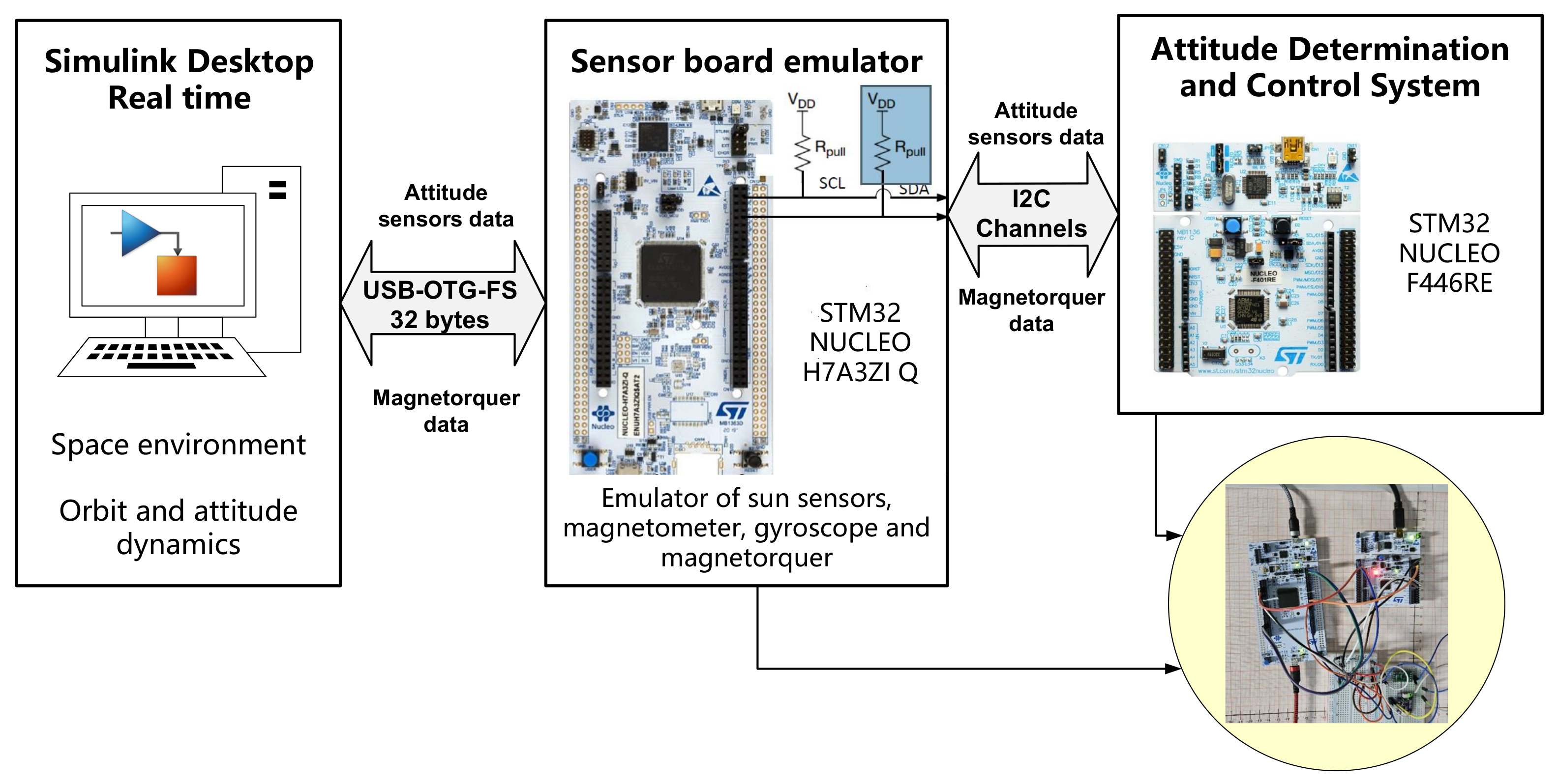
Software verification and validation are crucial prior to deploying a flight-ready CubeSat model. To facilitate this, a real-time sensor emulator is implemented to transmit sensor data simulated by Matlab/Simulink. This includes sensor noise and employs communication protocols such as USB and I2C.

The real-time emulator computer transmits sensor parameters to a sensor simulation block implemented on a developed board. This data is sent via I2C to an Attitude Determination and Control System (ADCS) block, which generates the 6-DOF CubeSat dynamics orbit data. This information is then relayed back to the developed board and forwarded to the simulation computer. The sensors used in the emulator include sun sensors, magnetometers, and gyroscopes.

For transmitting sensor simulation data, the USB OTG FS communication protocol is employed, supporting data transfer rates up to 12 Mbps in USB 1.1. This choice eliminates the need for additional hardware on the development boards, thereby optimizing energy consumption. In contrast, RS232, designed for long distances and transmitting up to 11,520 Bytes/s, is unsuitable for the proposed testbed. UDP, while faster, suffers from data loss and depends on network quality, making it unreliable. TCP, despite its high data security, introduces latency due to handshaking, making it non-deterministic for real-time simulation. Both UDP and TCP add complexity in programming for low latency and efficient data management, requiring extensive network management and significant memory buffers in MCUs. Additionally, the compatibility of development boards with TCP/IP Middleware for these protocols must be considered.

I2C is recommended for data transmission in sensor emulation due to its computing efficiency and minimal hardware requirements compared to other communication protocols, which may require more hardware and computing processes. For example, the CAN communication protocol, with speeds between 100 Kbps and 1 Mbps, requires additional hardware such as CAN transceivers and controllers, increasing energy consumption and space requirements.

The I2C communication protocol follows a structured approach: the simulation PC generates emulated data for the sensors (sun sensors SLCD-61N8 from Advanced Photonix, Tokyo, Japan, magnetometer MMC5603NJ from Memsic Inc., Tianjin, China, and gyroscope L3GD20 from STMicroelectronics, Geneve, Switzerland). Both the magnetometer MMC5603NJ and gyroscope L3GD20 have 16-bit resolution per axis (48 bits per measurement). Magnetometer and gyroscope measurements along the x, y, and z axes are multiplexed to two bytes each, resulting in a total of six bytes per measurement. Conversely, sun sensors SLCD-61N8 provide single measurements transformed into two bytes each. The total bytes transmitted are 12 bytes, combining data from the six sun sensors, magnetometer, and gyroscope. I2C is configured in interruption mode with a 400 kHz fast mode using a pull-up configuration with 4.3 K$\mathrm{\Omega }$ resistors. This configuration mitigates jitter by closely aligning with the expected data and reception timings, ensuring reliable communication over extended periods, as illustrated in Figure 8.

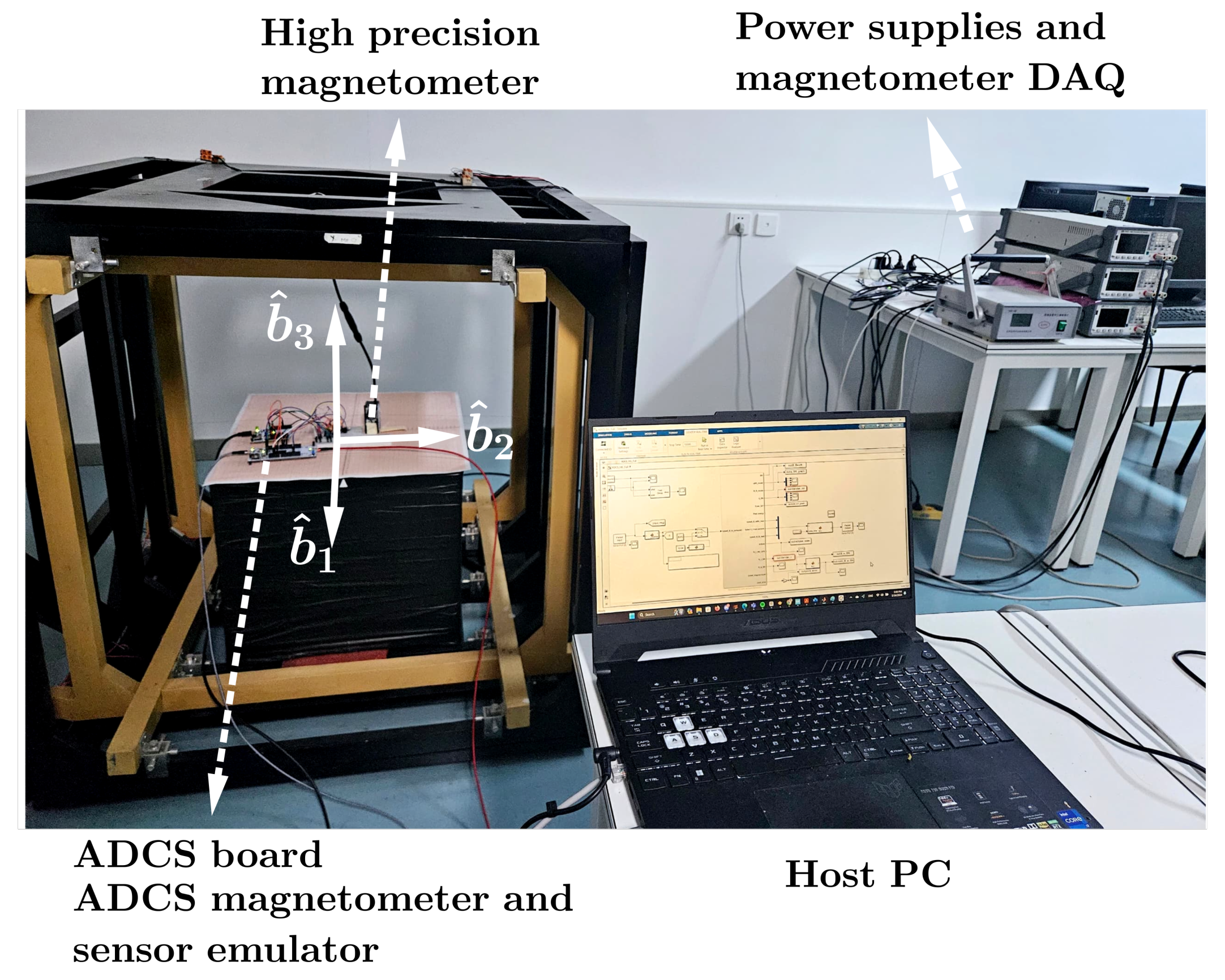
3.3.3. Helmholtz Cage Configuration for HIL

For HIL simulation, an approximation of Earth’s magnetic field is required. This was achieved using a high-precision magnetic testbed, the IS501NMTB, which boasts an accuracy of 99.89% in reproducing the desired magnetic field along the satellite’s orbit [13]. Additionally, the HSF-100 magnetometer was selected for measuring the magnetic field across the three axes, with the primary objective of calibrating and providing data every second. The magnetometer data were transmitted to the computer controller via USB and have their own data acquisition system.

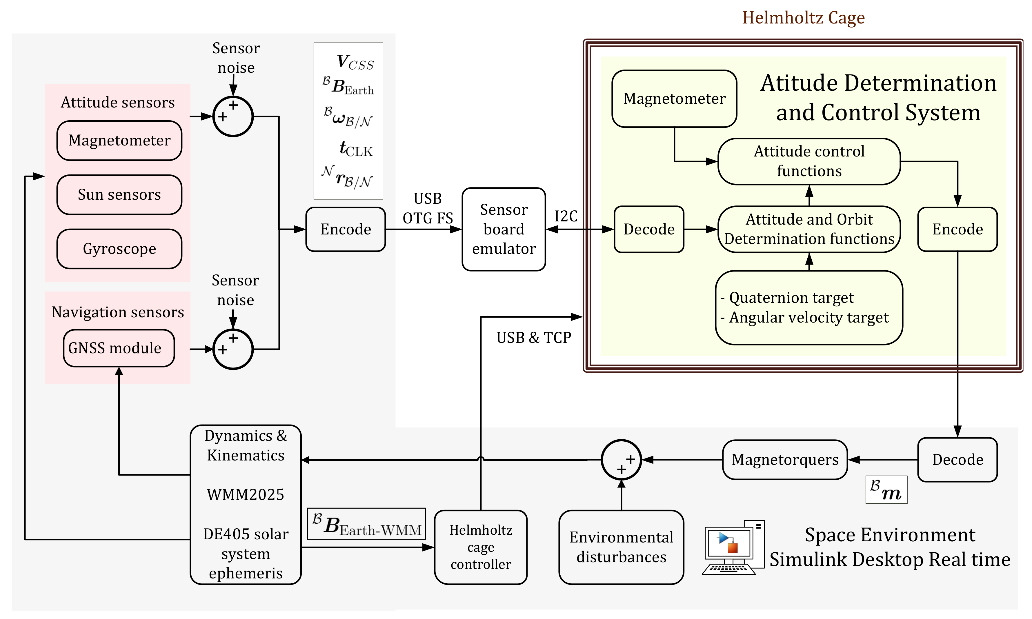
Furthermore, the TCP/IP protocol was employed for communications between the high-precision DC Sources and a router, which was connected to the computer via Ethernet. This setup necessitated prior knowledge of its IP address to send appropriate commands to power the Helmholtz coils. In addition, Simulink received an input of 27 strings, which contained the magnetic field measurements of HSF-100, which were converted into doubles, while the computer controller sent an output packet sized at 200 bytes. This packet included the voltage value and commands directed to the high-precision DC Sources. An example of an initial command sent includes functions such as start mode, command control mode, maximum current, delay, and initial voltage.

Furthermore, for calibration purposes, both the magnetic field and voltage were sent to the workspace to fit a linear model. This process enabled the determination of the necessary voltage required to achieve a specific magnetic field. Subsequently, in magnetic field control, a PID controller was employed to mitigate the offset inherent in the linear model. The input to the controller was the error signal, derived from the disparity between the actual magnetic field value measured by the magnetometer and the desired setpoint acquired from the WMM (World Magnetic Model) expressed in the CubeSat’s body frame $\mathcal{B}$. The physical configuration and schematic representation for the proposed testbed are shown in Figure 9 and Figure 10, respectively.

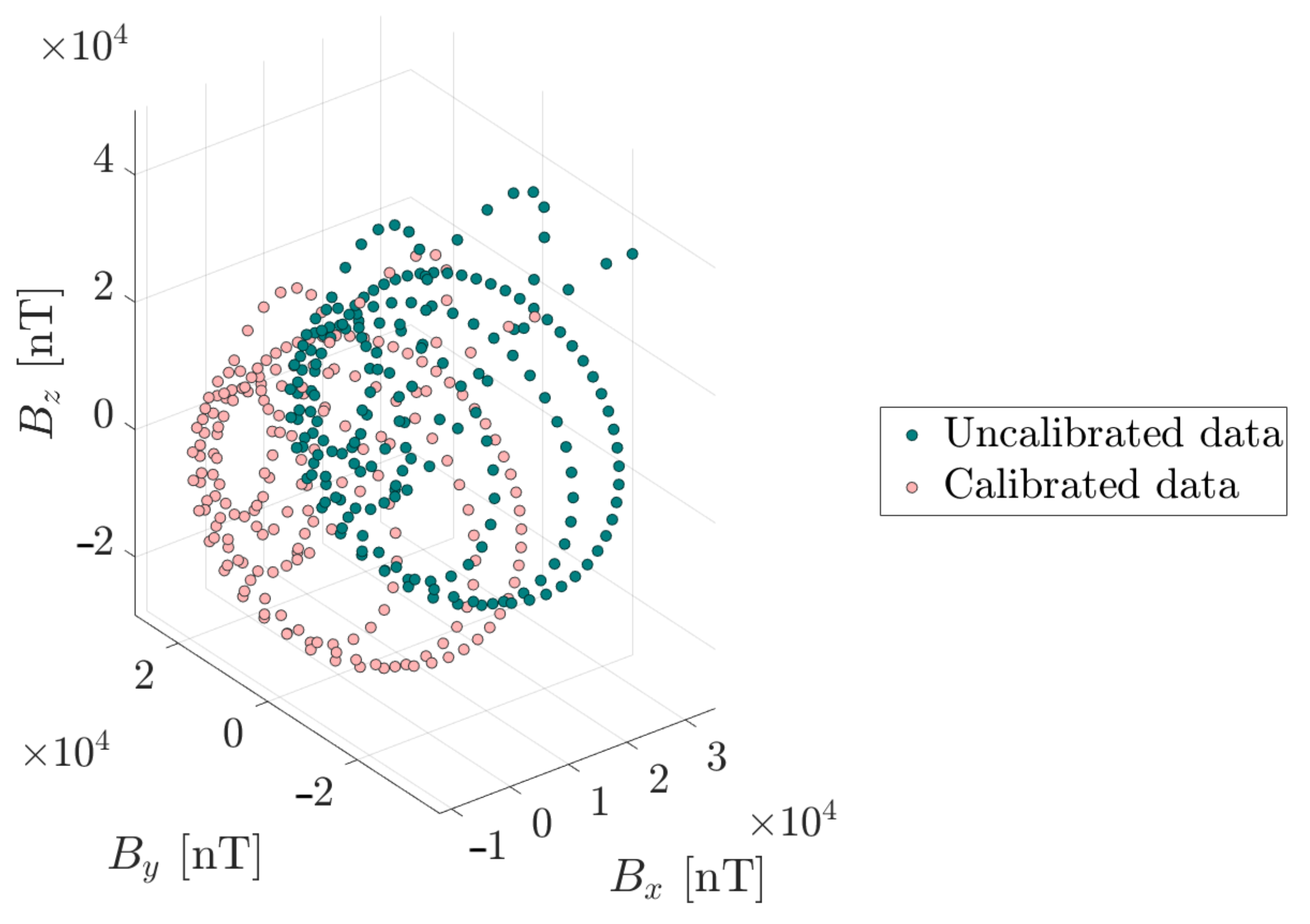
Finally, in order to enhance accuracy of magnetometer measurements, before conducting the HIL test, a magnetometer calibration was implemented via a fitting ellipsoid algorithm. Furthermore, taking advantage of the proposed testbed, an on-orbit calibration was conducted during the phase of detumbling control. Afterward, this calibrated data was utilized for the HIL test.

4. Results

The framework developed was oriented to complement the verification and validation process at the module level of the ADCS of a CubeSat 1U. Since each approach is different in execution and complexity, the following subsections will describe the contribution and results of each proposed approach.

4.1. Model-Based Verification for ADCS

Systems engineering for aerospace projects is based on general guidelines and standardized phases that guarantee the expected performance of a system for a defined problem. Therefore, the life cycle of a space project is divided into seven phases according to the specifications detailed in ECSS-M-ST-10-01. Each phase has associated review milestones, of which a “top-down” character is observed from the PRR to the PDR to satisfy in a general way the customer’s requirements. On the other hand, from the CDR to the RA milestones, a “bottom-up” behavior is observed, starting from the lowest-level supplier to the system operator. Consequently, a V-model is often used to describe the life cycle of this type of project.

The V-Model in this research is complemented with an early model-based V&V process which facilitates the detection and correction of errors from early design stages [51]. Therefore, the model-based approach in system development is fundamental for development time reduction and more rigorous testing [52]. In this context, the different model-based development approaches correspond to characteristic stages of the V-Model and the project phases and documentation specified in ECSS-M-ST-10C [53], as can be seen in Figure 11.

The initial stages of the cycle, from Phase 0 to Phase B, primarily concentrate on developing functional and technical requirements. This phase encompasses the identification of all activities and resources, and the initial assessment of technical risks leading up to the preliminary design. Within this framework, SIL (Software in the Loop) is proposed as a deliverable for the first development phase to verify the identified systems and initial risks. It is crucial to implement and validate the ideal simulation environment and the MIL (Model-in-the-Loop) environment beforehand to ensure accuracy.

Phase C advances to detailed system definition, incorporating detailed sensor and actuator models. In this phase, MIL is recommended to address the need for more comprehensive model analysis. SIL tests may also be revisited to ensure system integrity and performance. Phase D progresses further into the system’s implementation, where both PIL (Processor-in-the-Loop) and HIL (Hardware-in-the-Loop) methodologies can be employed. These methodologies facilitate a thorough analysis of the performance of not only the physical sensors but also the embedded controller, ensuring robust and reliable system performance.

4.2. Systematic Verification of the ADCS

The base or ideal simulation on which all the approaches proposed in this research are based has two test cases, one for detumbling by using B-dot control and the other for nadir pointing to execute the aforementioned Earth observation mission. Based on the proposed methodology, the specific roles of the different approaches and the results obtained are described below. Additionally, the contribution of each approach is detailed according to its specific contribution.

4.2.1. Source Code Verification and Performance Simulation

To verify the preliminary design of the controller algorithm, Software-in-the-Loop (SIL) results are presented in Figure 12. Monte Carlo simulations were conducted, where the control gains $K_d$ and $K_p$ were varied within a random uniform distribution, with a variation of 5.8% from their original values. This approach allowed for a comprehensive sensitivity analysis, evaluating the standard deviation, mean, and weighted sum of the pointing error. The results of this analysis are plotted in the subsequent graphs, with the z-axis representing the standard deviation, mean, and weighted sum of the pointing error, respectively. This detailed examination provides crucial insights into the performance and robustness of the controller algorithm under varying conditions.

As described in previous sections, the congruence of the code generation embedded in the Simulink model was verified using the Simulink C Caller function. The generated code was debugged to ensure that the simulation results of the simulated controller and the implemented controller were identical.

In

Table 4. Parameter sensitivity analysis, Monte Carlo/angular velocity/inertia matrix).

Parameters	Angular Velocity	Inertia Matrix
	x y z	Ixx Iyy Izz
Initial value	−0.001 0.003 0.002	1.6X10-17 1.3X10-17 1.4X10-17
Final value	0.004 0.008 0.007	1X10-7 1X10-7 1X10-7
Mean	0.003 0.001 0.001	1X10-7 1X10-7 1X10-7
Sampling method	Random	Random
Distribution	Uniform	Uniform

, the data introduced into Simulink/Sensitivity Analysis for developing the Monte Carlo study for angular velocity and inertia matrix are shown. For this purpose, it is necessary to input an initial value and the mean for the normal uniform distribution. The Monte Carlo method will generate random values within the range of the initial and final values. The initial values for angular velocity and inertia matrix introduced are stable values during the Simulink simulation for the required orbit.

The data introduced for sensitivity analysis for Euler angles and initial CubeSat orbit condition are shown in

Table 5. Parameter sensitivity analysis, Monte Carlo/Initial CubeSat orbit condition/Euler angles).

Parameters	Initial Cubesat Orbit Condition	Euler Angles
	$\theta$	x y z
Initial value	0	45 −45 45
Final value	360	360 360 360
Mean	0.1	0.1 0.2 0.3
Sampling method	Random	Random
Distribution	Uniform	Uniform

.

In Figure 13, the mean pointing accuracy from Monte Carlo simulations is shown, accounting for variations in angular velocity, initial orbit conditions, and initial rotation Euler angles. This illustrates the controller’s average performance across different scenarios. On the other hand, Figure 14 presents the standard deviation of pointing accuracy, highlighting the variability and robustness of the system. It demonstrates how consistently the controller maintains performance given the same variations in initial conditions. These results provide a comprehensive evaluation of the controller’s reliability and effectiveness under diverse operational scenarios.

The response of the pointing error to different initial angular velocities is depicted in Figure 15; during the Monte Carlo simulation the initial angular velocity ${}^{\mathcal{B}}{\mathit{\omega }}_{\mathcal{B}\mathcal{N}}\left(0\right)$ along the x, y, and z axes was taken as $\left[\begin{array}{ccc}-0.001& 0.003& 0.002\end{array}\right]$ radians, respectively; then, it was varied by adding an offset. Therefore, the range of angular velocity variation is $\left[\begin{array}{ccc}-0.001& 0.003& 0.002\end{array}\right]$ to $\left[\begin{array}{ccc}0.004& 0.008& 0.007\end{array}\right]$; the data depicted on the x-axis are the normal resultant of the initial angular velocity range. The attitude stability of the CubeSat is affected by this range of angular velocity, determining how the CubeSat responds to external disturbances; this range also influences the response and performance of the ADCS in maintaining a stable attitude under different angular velocities.

Otherwise, CubeSat’s inertia matrix was approximated using Solidworks, obtaining the following:

$$\left[I_{\mathcal{B}}\right]=\left[\begin{array}{ccc}1556542.74& 18844.31& -25.84\\ 18844.31& 1337462.20& -2447.28\\ -25.84& -2447.28& 1408210.65\end{array}\right]\times {10}^{-9}[\mathrm{Kg}·{\mathrm{m}}^2]$$

So, variation in the inertia matrix is depicted in Figure 16; depicted on the x-axis is the offset value that is added to the moments of inertia (the diagonal of the inertia matrix ${\mathit{I}}_{\mathcal{XX}}$, ${\mathit{I}}_{\mathcal{YY}}$, ${\mathit{I}}_{\mathcal{ZZ}}$). Hence, the variation in the inertia matrix is in the range of $(1\times {10}^{-3}\le variation\le 5\times {10}^{-3})$, applied to the initial moment of inertia: ${\mathit{I}}_{\mathcal{XX}}=\left[\begin{array}{c}1.556\times {10}^{-15}\end{array}\right]$; ${\mathit{I}}_{\mathcal{YY}}=\left[\begin{array}{c}1.337\times {10}^{-15}\end{array}\right]$; ${\mathit{I}}_{\mathcal{ZZ}}=\left[\begin{array}{c}1.408\times {10}^{-15}\end{array}\right]$.

This variation was carried out to analyze the possible disturbances and variations within the construction and manufacturing process of the CubeSat, or the degradation of the CubeSat structure over time, resulting in a variation in control performance.

The initial 3-1-3 Euler angles regarding the initial frame $\left[BN\right]\left(0\right)$ suffer a variation in each axis in a range of $(0\le degrees\le 360)$ trying to cover all possible rotations; the initial pointing error for each normal resultant of the Euler vector is depicted in Figure 17; in this way it is possible to observe the performance of ADCS with respect to the change in initial rotation verifying the mean of the pointing error depicted on the y-axis.

Afterward, the variation in the perigee argument in orbit elements is depicted in Figure 18. So, the range of perigee ($\mathit{\omega }$) is $(0\le perigeeargument\le 360)$ degrees in the Monte Carlo simulation; the inclination and ascending node remain constants to obtain a circular orbit; the values of the ascending node and inclination for an optimal orbit that crosses Bolivian territory are $[\mathbf{16};\mathbf{30};\mathit{\omega }]$, respectively.

4.2.2. Model-Based Functionality Performance

Before presenting the results, the test conducted for on-orbit calibration is shown in Figure 19. The data were gathered during the detumbling maneuver. Note that the calibrated values were used for the HIL test. It is important to highlight that, ideally, the best data acquisition for magnetometer calibration should encompass all possible 3D rotations. However, the conducted test is intended to be representative, and further studies could be conducted using the proposed framework for simulating on-orbit calibration.

Subsequently, a comparison of the complete attitude determination was conducted for Bdot and nadir, as depicted in

Table 6. Model-based performance results for nadir (calculated after 2 orbits).

Simulation Approach	Pointing Accuracy, Mean Value	Pointing Accuracy, Standard Deviation
SIL	21.4017	7.2141
MIL	11.6914	3.5952
PIL	18.2179	6.1331
HIL	9.9649	2.8167

and

Table 7. Model-based performance results for Bdot (calculated after 2 orbits).

Simulation Approach	Angular Velocity Norm, Mean Value	Angular Velocity Norm, Standard Deviation
SIL	0.0022	1.2858 × ${10}^{-4}$
MIL	0.0022	1.3972 × ${10}^{-4}$
PIL	0.0022	1.3705 × ${10}^{-4}$
HIL	0.0024	1.4217 × ${10}^{-4}$

, in order to estimate their respective performance in evaluating the mean pointing accuracy, which should tend towards zero, and minimize the standard deviation. In Figure 20, a comparison of the Bdot controller’s initial angular velocities with $\left[\begin{array}{ccc}-0.01& 0.03& 0.02\end{array}\right]$ [rads/s] and in Figure 21 the nadir controller with $K_p=0.00013555$, $K_d=0.0743$, and $\left[\begin{array}{ccc}-0.001& 0.003& 0.002\end{array}\right]$ [rads/s] radians is presented. The quality control for both controllers spans two orbits.

For HIL simulation, latencies of 5.2 ms and 15 ms are observed for Bdot and nadir, respectively. This contrasts with PIL, where latencies of 4 ms and 12 ms are recorded for the same controllers. The reported computational resources post-code generation for the STM32F446RE, used for PIL validation, show a RAM usage of 32.2 KB out of 128 KB and a flash memory usage of 141.99 KB out of 512 KB. Conversely, the HIL test shows a RAM usage of 34.27 KB out of 128 KB and a flash memory usage of 142.57 KB out of 512 KB.

5. Discussion

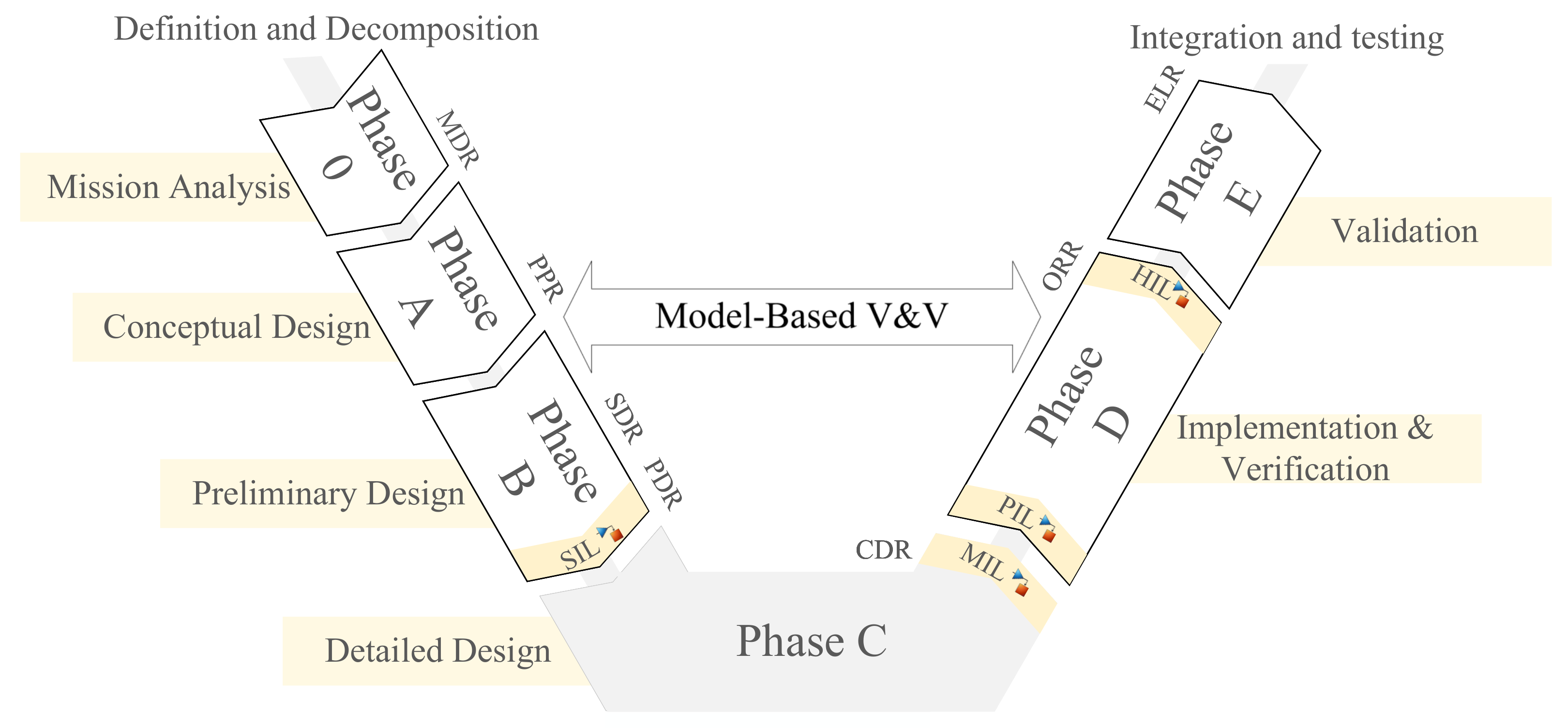
Models are widely used in different areas of spacecraft design, whereas simulation is a key element in supporting the engineering and operational activities of space systems. In this regard, System Modeling and Simulation (M&S) is considered a system-level support discipline. This discipline encompasses the simulation models and infrastructure to support specification, design, and the entire Verification and Validation (V&V) process. Given the importance of maximizing the benefits of their use, the European Space Agency (ESA) has established a Technical Memorandum to cover the modeling and simulation facilities required to support all these system-level activities: ECSS-E-ST-10-21A. Standard “Systems Engineering: System modelling and simulation”. In this research, this analysis is further explored, not only at the system level related to the space segment or ground segment, but also at the module and component level. This approach introduces early-stage testing for initial phases of development specifically for the ADCS module, specifying details on facilities and interfaces.

During the development process, models are also supposed to mature in order to support system–engineering trade-offs. In the first stage of the project, as seen in [25], a System Concept Simulator (SCS) was developed for fast evaluation and system design concepts since it was not running in real time. Nevertheless, this research went a step further into a Functional Engineering Simulator (FES) that allows us to verify critical elements of the baseline system proposed, reusing mathematical models of the SCS and adding details to it as seen in the MIL approach. Finally, these simulators prepared the basis for the Functional Validation Testbench (FVT) to support the analysis of the system performance and the V&V process of critical components as seen in SIL, PIL, and HIL. Additionally, this paper introduces a methodology based on V-cycle for project development at a module level for the ADCS. Since no uniform methodology is established in the ECSS-E-ST-10-21A for this level of development at early stages, this research complements a standard methodology for the design process that could be characterized by the designer’s necessities based on the model-based design.

Delving into the contribution of each simulation environment to the design and V&V process, this process started with the extension of the SCS previously developed. Detailed models of the space environment and also of the sensors and actuators were included in order to obtain more realistic results considering jitter, noise, and data handling between the space environment and the controller as seen in MIL. These models were included in all the simulation environments which allowed us to analyze not only the controller performance in each environment but also the effects of the embedded capabilities and computational resources in the performance of the controller. In this sense, it could be seen that the controller executed on board in real time never exceeded 24.06% of the memory capacity and 19.44% of the RAM capacity executed in PIL and HIL environments. Given that the computational capabilities of the microcontrollers are not exceeded, it can be seen that there is no relationship between the capacity usage and the controller performance as seen in Table 6 for nadir pointing and in Table 7 for detumbling.

The originally proposed framework is applicable for the validation of any control system that includes a magnetometer as attitude sensor. Moreover, the scalable potential of this framework allows its adaptation to validate systems of higher volume and complexity due to the modularity and flexibility of the proposed system, allowing developers to include in the simulation the dynamics of the analyzed spacecrafts and mathematical models of sensors or actuators, or even to physically implement other sensors, which also involves modifying the controlled environment to obtain reliable results. In addition, the versatility of the proposed approach provides the necessary tools to implement code generation using SIL and PIL in embedded systems with low computational resources, assuming that the sensor readings are performed directly by the controller and considering the restrictions discussed in Section 3.2, such as the alignment of sampling times between the simulation and the controller, as well as that the controller board supports C99 (ISO), to ensure the consistency of the model and its corresponding code.

Based on the HIL environment, the on-orbit calibration task was also simulated and executed, since the magnetometer is supposed to obtain accurate data once in orbit. In addition, the magnetometer was calibrated considering external and internal errors modeled with a robust algorithm. Subsequently, the algorithm was run during detumbling mode, so that the physical magnetometer was able to collect data in all axes simulating on-orbit performance.

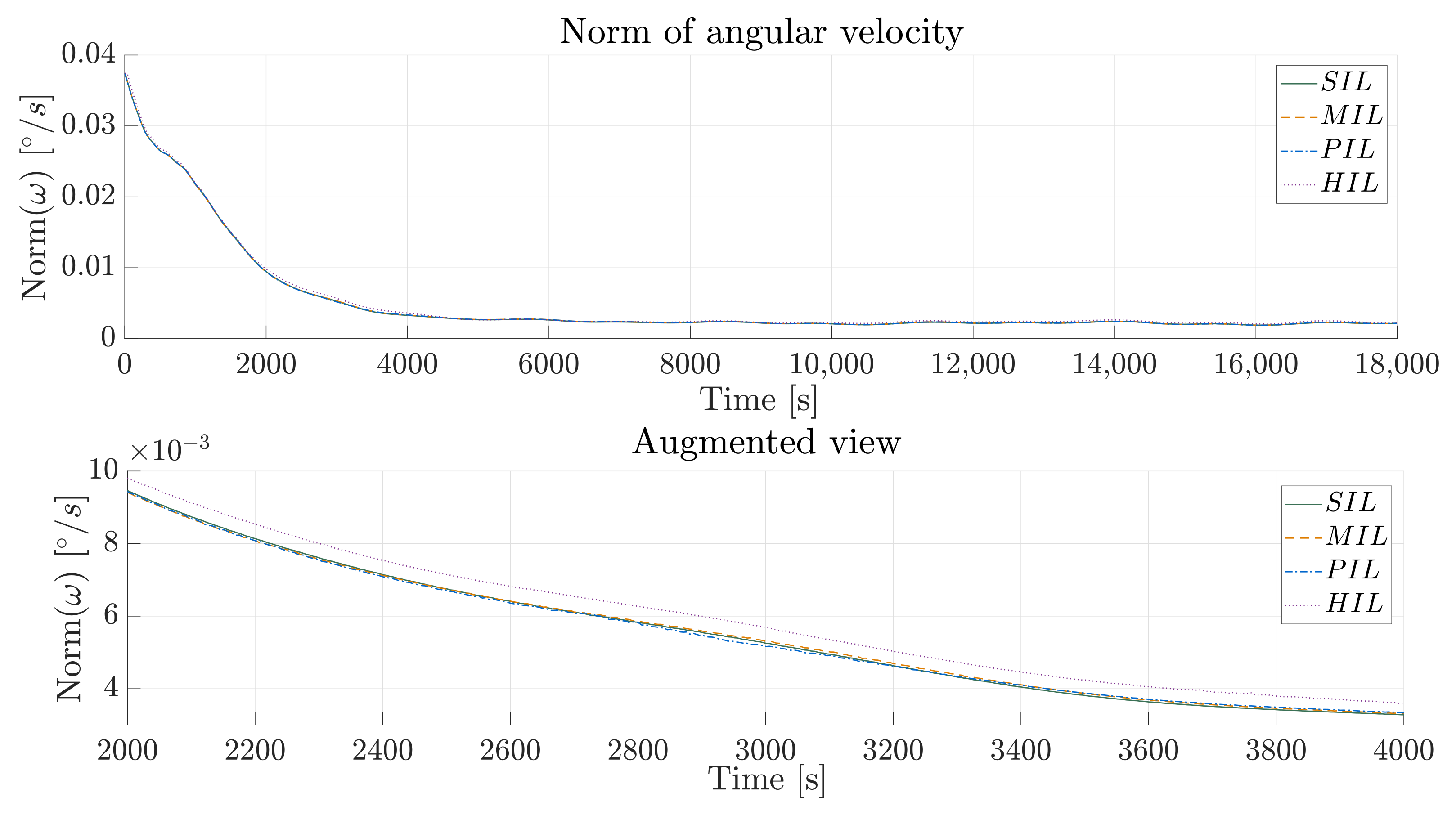
Given that the same controller was executed in all the environments and in the same conditions, a clear relationship between the high latency in HIL (4 ms and 12 ms) and the performance of the B-dot controller could be inferred due to its high angular velocity resultant seen in Figure 20, resulting in an error of approximately 0.07% compared to MIL. As a result, to increase the fidelity of HIL, the latency must be reduced in order to obtain significant results. The accuracy of SIL decreases compared to MIL, possibly because dedicated Simulink blocks optimize the MIL environment. The use of the “C Caller” block in SIL can introduce dependencies that result in algebraic loops, negatively affecting the accuracy and performance of the simulation.

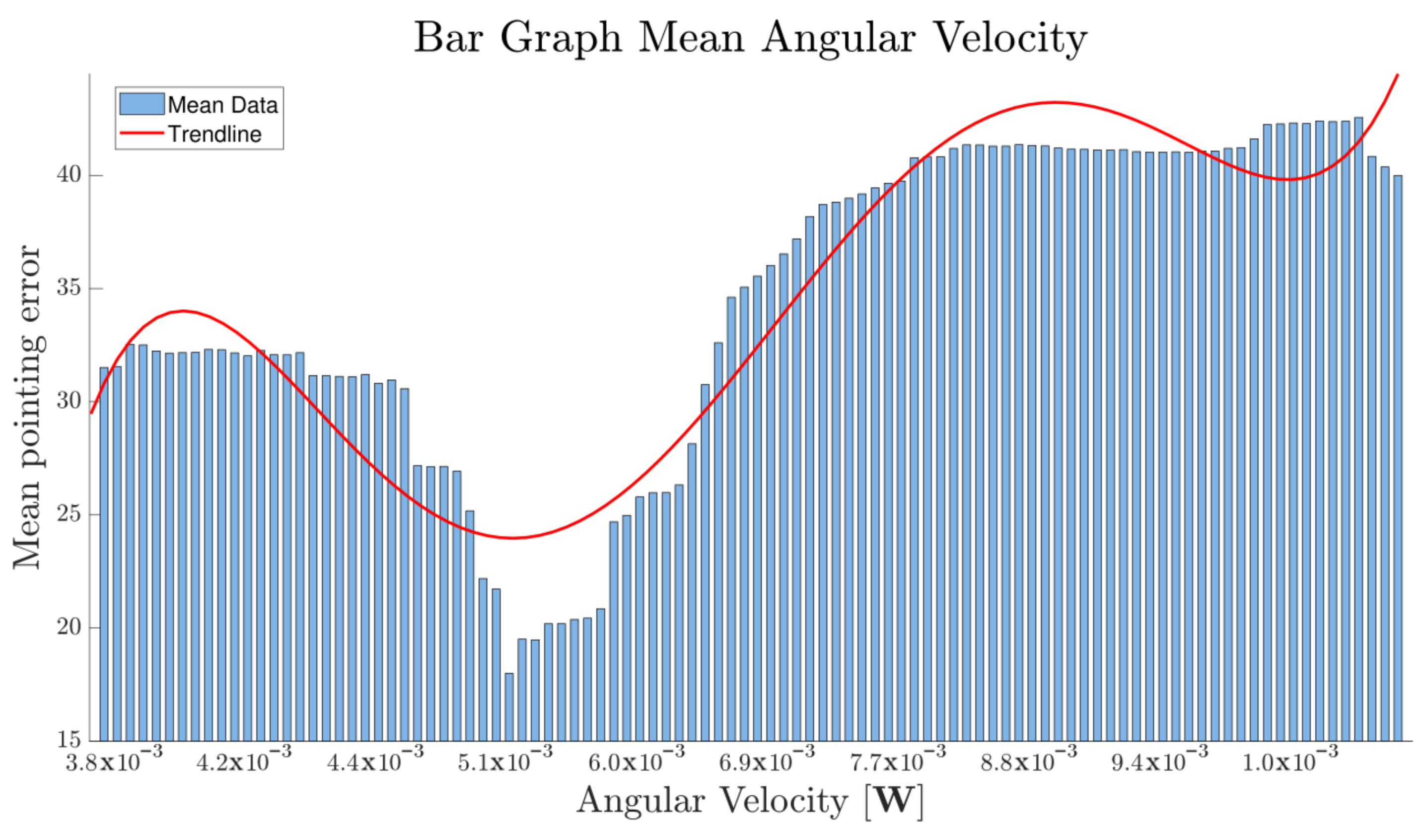
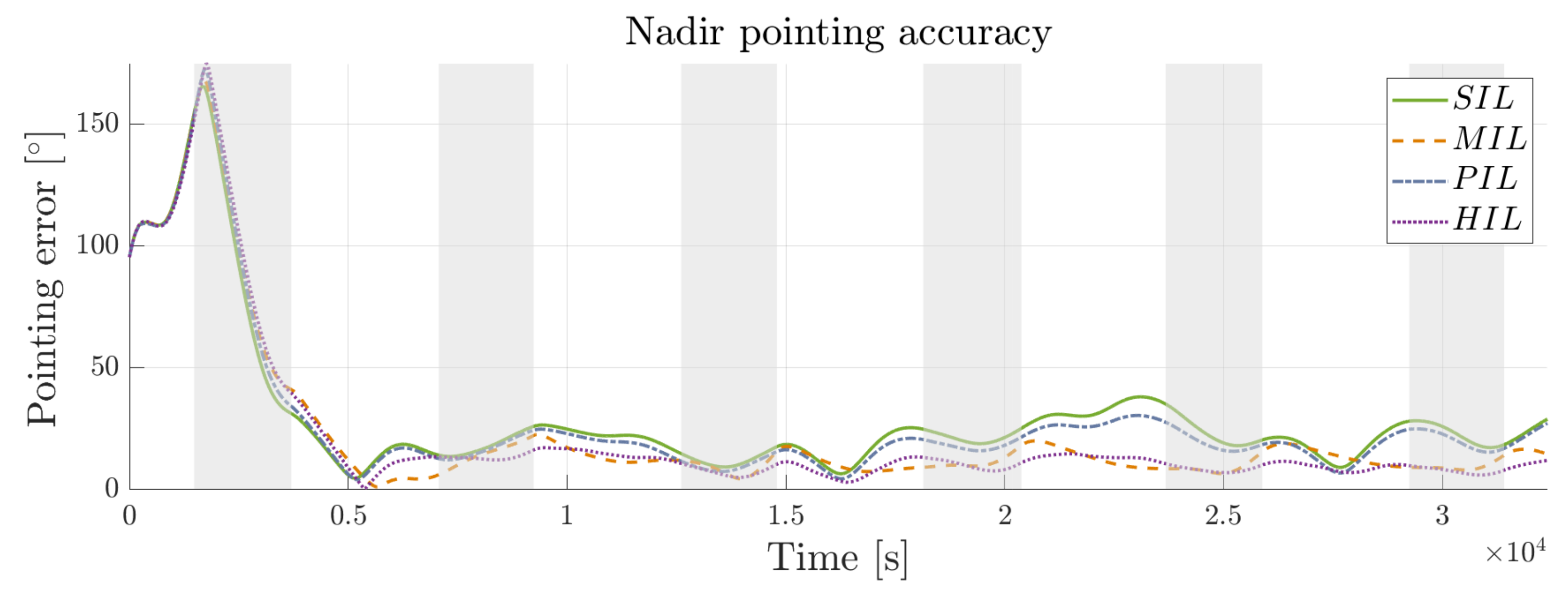
Regarding the performance of the evaluated controller, SIL stands out as an ideal simulation environment to establish the initial optimal conditions, since its performance is not influenced by other hardware. Taking advantage of this characteristic, the sensitivity analysis was conducted to obtain the most optimal control gains to minimize the pointing accuracy error in nadir pointing. The sensitivity analysis using Monte Carlo provided an insightful approach to the effect of the initial conditions of the simulated environment on the performance of the controller. In this regard, starting with a high initial angular velocity requires increased effort from the actuators, leading to a higher pointing error as seen in Figure 15. As angular velocity decreases, the error should also decrease. Nevertheless, small fluctuations in the velocity make the error increase. It must be noted that this phenomenon could be caused by factors of the system dynamics model, such as numerical method inaccuracies, sensor reading anomalies prevalent at exceedingly low velocities, sampling noise, Gaussian perturbations, or, predominantly, quantization effects inherent to bit resolution.

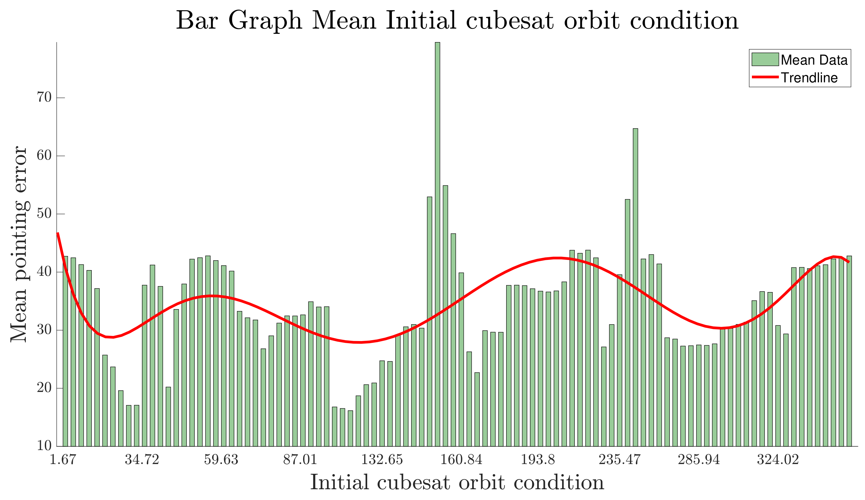
Furthermore, variations in the CubeSat inertia also increase the pointing error as seen in Figure 16. Even though changing the inertia of a CubeSat on orbit could be possible only by degeneration of the nanosatellite, this approach is useful for considering new control configurations if the physical design is changed during the development process. Indeed, it is necessary to measure the center of mass, center of inertia, and mass of the satellite to adjust the initial algorithm to meet the requirements of the launcher. Once the launcher has been chosen, adjustment of the structure design can be made from the original design, affecting the mass properties of the CubeSat and subsequently the controller. In this regard, model-based design is necessary for analyzing the possible impact of making minor changes in the design without necessarily implementing those changes. Even though inertia is critical for the system performance, it is not a variable that could be easily set by the developers. Alternatively, the initial orbit parameters are variables that could be set by the deployers. 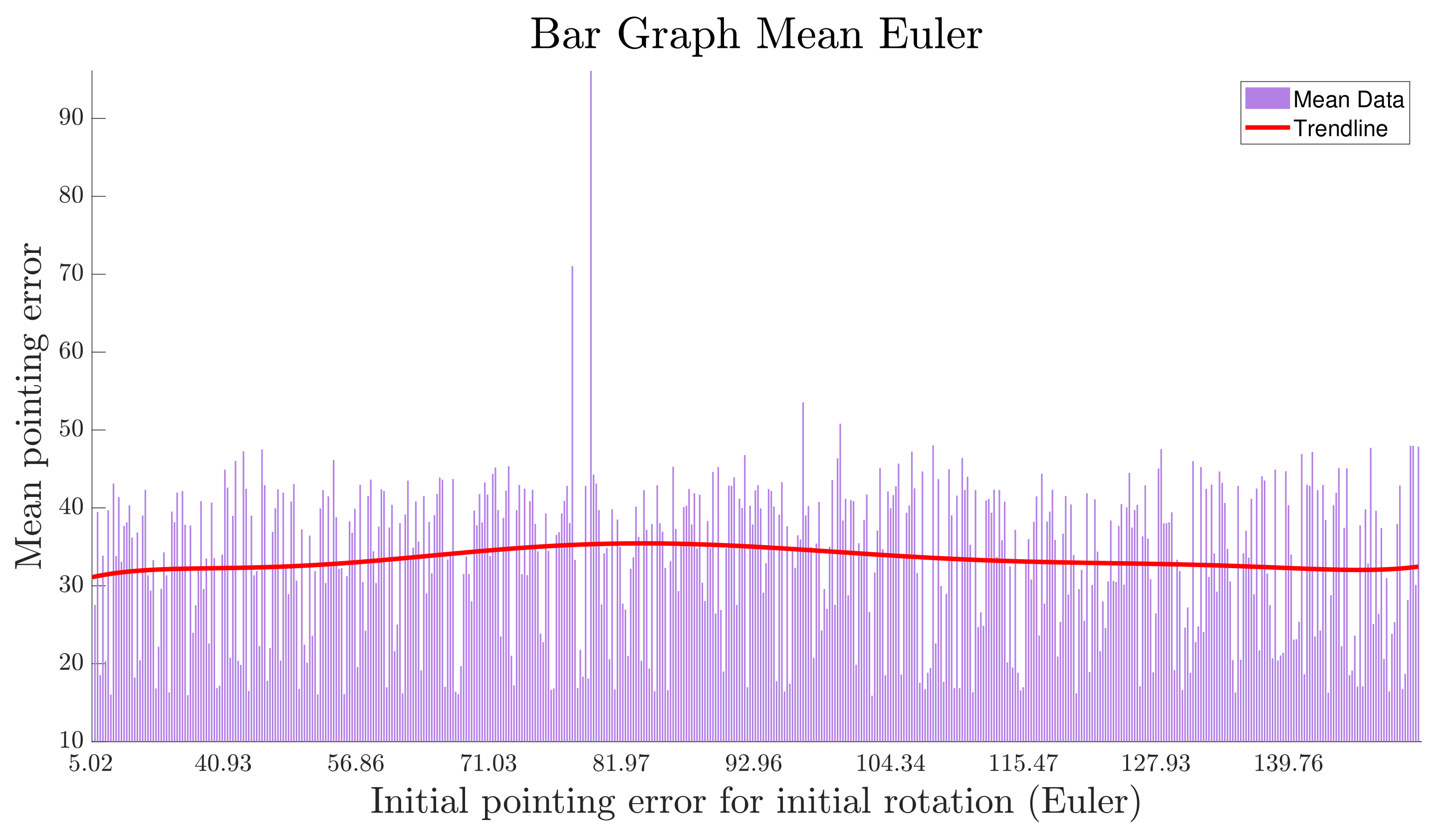Thus, the selection of the deployer could be guided to approximate an optimal selection based on Monte Carlo analysis, since the simulation demonstrates that the most optimal points for the controller to begin acting occur at approximately 34.72 and 109.83 degrees, resulting in a mean pointing error of less than 20 degrees, as seen in Figure 18. Finally, from the results shown in Figure 17, it could be inferred that the pointing error in nadir control tends to remain constant for the simulated initial pointing error during two orbits, highlighting the importance of optimally completing the detumbling state to less than 0.1$°$/s as seen in Figure 1 to decrease the pointing error once the state is changed.

As could be seen, each approach is limited by their own configurations, and also contributes significantly to the understanding and analysis of the whole system performance. Hence, all simulation environments are complementary to perform an enhanced model-based design and also to carry out a comprehensive V&V process.

6. Conclusions and Future Directions

This article presents an in-depth analysis of four different simulation environment configurations, utilizing a model-based methodology to verify and validate the ADCS from the early stages of development. This approach supports both the design and implementation of modular systems, contributing significantly to the standard systems-focused methodology. Each simulation environment is detailed to illustrate the specific requirements and facilities necessary for effective validation. The sequential approach enables designers to isolate and differentiate errors arising from mathematical modeling, computational limitations, and physical implementation. This process is particularly advantageous for solving specific problems and optimizing the Verification and Validation process.

In Section 3.2, the SIL environment was utilized for optimizing the controller through sensitivity analysis. This step allowed for the identification of optimal control gains and the evaluation of the system’s response to various initial conditions. SIL simulations showed that, by varying the control gains $Kd$ and $Kp$ within a 5.8% range, the mean pointing accuracy and standard deviation of the pointing error were effectively assessed, revealing a consistent performance across different scenarios. Section 3.1 introduced detailed models of physical components and the simulated environment to assess their impact on controller performance, serving as a verification method after the detailed design of the controller, typical of phase C in the standard design process. Despite the error margin in SIL due to dependencies and algebraic loops, it remains an ideal simulation method as it is unaffected by hardware inconsistencies. The MIL environment allowed for evaluating the controller’s performance, showing a mean pointing accuracy of 11.6914° with a standard deviation of 3.5952° for nadir pointing and an angular velocity norm of 0.0022 rad/s with a standard deviation of 1.3972 × ${10}^{-4}$ rad/s for detumbling.

Using the PIL simulations described in Section 3.3.1, variables such as latency and memory usage were isolated to analyze their effects on controller performance. PIL simulations showed a slight increase in latency (4 ms for B-dot and 12 ms for nadir) and a mean pointing accuracy of 23.3497° with a standard deviation of 7.8226° for nadir pointing and an angular velocity norm of 0.0022 rad/s with a standard deviation of 1.3705 × ${10}^{-4}$ rad/s for detumbling. This step is crucial for understanding the impact of computational constraints on the embedded system. The HIL environment, also discussed in Section 3.3.1, provided insights into the latency impacts on system performance. HIL simulations indicated higher latencies (5.2 ms for B-dot and 15 ms for nadir) but still maintained comparable performance, with a mean pointing accuracy of 9.9649° and a standard deviation of 2.8167° for nadir pointing, and an angular velocity norm of 0.0024 rad/s with a standard deviation of 1.4217 × ${10}^{-4}$ rad/s for detumbling. The HIL environment accurately approximated real behavior, allowing for effective comparisons with other simulation environments.

Depending on the specific characteristics of a CubeSat, it is necessary to take into account all risk components implicating new technologies, mobile parts or, in this case, COTS components. As a matter of fact, rigorous testing using specialized test environments is necessary after integration to assess system functionality and operational expectations. First of all, due to the usage of COTS, rigorous thermal testing must be performed, while all modes of operation of the ADCS must be tested to verify its performance under extreme temperature variations. Further, outgassing tests should then be considered to evaluate COTS degradation and its performance under vacuum conditions and during operation. In addition, vibration and acoustic tests should also be performed to validate the internal connections and their potential hazard due to mechanical disturbance generated by the rocket. In addition, the influence of electromagnetic interference between on-board equipment should be evaluated through electromagnetic compatibility (EMC) tests, since accurate magnetic field measurements are a priority for this mission. Moreover, EMC tests should be performed between the nanosatellite and the launch vehicle to ensure there is no electromagnetic interference with the telecommunications system of the rocket. All these additional tests must be performed prior to launch in dedicated facilities to meet all technical and operational requirements.

The proposed workflow aims to provide designers with a comprehensive analysis of the module and its components, making it a valid approach for early design stages. Future work will focus on the sequential integration of additional physical components and the implementation of a more complete physical environment for systematic analysis of the entire ADCS. This will lay the foundation for moving towards Mission Performance Simulators, enabling verification of overall performance from the user’s perspective at the system level. Additionally, this approach could be adapted to other subsystems such as the telemetry, tracking, and command (TT&C) subsystem, to test localization capabilities (GPS) and support antenna selection decisions. This comprehensive approach ensures that CubeSat missions can achieve higher levels of reliability and performance, thereby enhancing the success rate of these missions.

References

1. Wu, S.; Chen, W.; Cao, C.; Zhang, C.; Mu, Z. A multiple-CubeSat constellation for integrated earth observation and marine/air traffic monitoring. Adv. Space Res. 2021, 67, 3712–3724. [Google Scholar] [CrossRef]
2. Daniel, V.; Inneman, A.; Marsikova, V.; Oberta, P.; Pina, L.; Hudec, R. CubeSat microsatellite demonstrator with X-ray optical payload. In Proceedings of the EUV and X-ray Optics: Synergy between Laboratory and Space VIII, Prague, Czech Republic, 26–27 April 2023; SPIE: Bellingham, WA, USA, 2023; Volume 12576, pp. 25–28. [Google Scholar]
3. Lepcha, P.; Malmadayalage, T.D.; Örger, N.C.; Purio, M.A.; Duran, F.; Kishimoto, M.; El-Megharbel, H.A.; Cho, M. Assessing the Capacity and Coverage of Satellite IoT for Developing Countries Using a CubeSat. Appl. Sci. 2022, 12, 8623. [Google Scholar] [CrossRef]
4. Aswin, M.; Pavithran, A.; Mangrole, Y.; Ravi, B. Structural and Thermal Analysis of a CubeSat. In Proceedings of the Conference of Innovative Product Design and Intelligent Manufacturing System, Rourkela, India, 25–26 November 2022; Springer: Berlin/Heidelberg, Germany, 2022; pp. 363–371. [Google Scholar]
5. Bloser, P.; Murphy, D.; Fiore, F.; Perkins, J. CubeSats for gamma-ray astronomy. In Handbook of X-ray and Gamma-ray Astrophysics; Springer: Berlin/Heidelberg, Germany, 2024; pp. 2215–2246. [Google Scholar]
6. Salem, N.A.D.M.; Hussein, A.I.; Mabrook, M.M. A proposed Array of Quadrifilar Helix Antenna for CubeSat applications. In Proceedings of the 2023 20th Learning and Technology Conference (L&T), Jeddah, Saudi Arabia, 26 January 2023; IEEE: Piscataway, NJ, USA, 2023; pp. 171–175. [Google Scholar]
7. ISO 19683:2017; Space Systems—Design Qualification and Acceptance Tests of Small Spacecraft and Units. International Organization for Standardization: Geneva, Switzerland, 2017.
8. ECSS-E-ST-10-03C; Space Engineering: Testing. European Cooperation for Space Standardization: Noordwijk, The Netherlands, 2012.
9. Cervettini, G.; Pastorelli, S.; Park, H.; Lee, D.Y.; Romano, M. Development and Experimentation of a CubeSat Magnetic Attitude Control System Testbed. IEEE Trans. Aerosp. Electron. Syst. 2021, 57, 1345–1350. [Google Scholar] [CrossRef]
10. Farissi, M.S.; Carletta, S.; Nascetti, A.; Teofilatto, P. Implementation and Hardware-In-The-Loop Simulation of a Magnetic Detumbling and Pointing Control Based on Three-Axis Magnetometer Data. Aerospace 2019, 6, 133. [Google Scholar] [CrossRef]
11. Kiesbye, J.; Messmann, D.; Preisinger, M.; Reina, G.; Nagy, D.; Schummer, F.; Mostad, M.; Kale, T.; Langer, M. Hardware-In-The-Loop and Software-In-The-Loop Testing of the MOVE-II CubeSat. Aerospace 2019, 6, 130. [Google Scholar] [CrossRef]
12. Tapsawat, W.; Sangpet, T.; Kuntanapreeda, S. Development of a hardware-in-loop attitude control simulator for a CubeSat satellite. IOP Conf. Ser. Mater. Sci. Eng. 2018, 297, 012010. [Google Scholar] [CrossRef]
13. Uscategui, J.; Wang, X.; Cuba, G.; Guarirapa, M. High-Precision Magnetic Testbed Design and Simulation for LEO Small-Satellite Control Test. Aerospace 2023, 10, 640. [Google Scholar] [CrossRef]
14. Shim, H.; Kim, O.J.; Park, M.; Choi, M.; Kee, C. Development of Hardware-in-the-Loop Simulation for CubeSat Platform: Focusing on Magnetometer and Magnetorquer. IEEE Access 2023, 11, 73164–73179. [Google Scholar] [CrossRef]
15. Hanafi, A.; Moutakki, Z.; Karim, M.; Rachidi, T. Effective Model-Based Systems Engineering framework for academic nanosatellite project management and design. CEAS Space J. 2024, 1–21. [Google Scholar] [CrossRef]
16. Nurgizat, Y.; Ayazbay, A.A.; Galayko, D.; Balbayev, G.; Alipbayev, K. Low-Cost Orientation Determination System for CubeSat Based Solely on Solar and Magnetic Sensors. Sensors 2023, 23, 6388. [Google Scholar] [CrossRef]
17. Ali, H.; Islam, Q.u.; Mughal, M.R.; Mahmood, R.; Anjum, M.R.; Reyneri, L.M. Design and Analysis of a Rectangular PCB Printed Magnetorquer for Nanosatellites. IEEE J. Miniaturization Air Space Syst. 2021, 2, 105–111. [Google Scholar] [CrossRef]
18. Khan, S.A.; Ali, A.; Shiyou, Y.; Tong, J. Reconfigurable Asymmetric Embedded Magnetorquers for Attitude Control of Nanosatellites. IEEE J. Miniaturization Air Space Syst. 2021, 2, 236–243. [Google Scholar] [CrossRef]
19. Arent, K.; Domski, W.; Cholewiński, M. Deployment of model based robotic control algorithms, designed using Matlab/Simulink, in the form of OROCOS components operating under Linux Xenomai. In Proceedings of the 2015 20th International Conference on Methods and Models in Automation and Robotics (MMAR), Miedzyzdroje, Poland, 24–27 August 2015; pp. 632–637. [Google Scholar] [CrossRef]
20. Nicola, C.; Nicola, M. Real Time Implementation of the PMSM Sensorless Control Based on FOC Strategy. In Proceedings of the 2022 4th Global Power, Energy and Communication Conference (GPECOM), Cappadocia, Turkey, 14–17 June 2022. [Google Scholar] [CrossRef]
21. Hsieh, J.H.; Huang, J.Y.; Yen, T.; Lee, S.; Chang, A.; Hou, L. Attitude Control Calibration and Experiment Testbed to Characterize Attitude Determination and Control System Performance. In Proceedings of the Small Satellite Conference, Logan, UT, USA, 19 August 2022; Available online: https://digitalcommons.usu.edu/smallsat/2022/all2022/302/ (accessed on 15 May 2024).
22. Pan, D.; Li, J.; Jin, C.; Liu, T.; Lin, S.; Li, L. A New Calibration Method for Triaxial Fluxgate Magnetometer Based on Magnetic Shielding Room. IEEE Trans. Ind. Electron. 2020, 67, 4183–4192. [Google Scholar] [CrossRef]
23. Modenini, D.; Bahu, A.; Curzi, G.; Togni, A. A Dynamic Testbed for Nanosatellites Attitude Verification. Aerospace 2020, 7, 31. [Google Scholar] [CrossRef]
24. Nieto-Peroy, C.; Palmerini, G.; de Oliveira, E.J.; Gasbarri, P.; Sabatini, M.; Milz, M. Simulation of Spacecraft Formation Maneuvers by means of Floating Platforms. In Proceedings of the 2021 IEEE Aerospace Conference (50100), Big Sky, MT, USA, 6–13 March 2021; pp. 1–10. [Google Scholar] [CrossRef]
25. Ticona, F.; Rojas, G.; Vidaurre, K.; Conchari, C.; Manrique, R.; Aliaga, N.; Condori, J. Attitude Determination and Control System for Nadir Pointing and Detumbling Using Magnetorquer for 1U Bolivian Cubesat. In Proceedings of the 2022 International Conference on Control, Robotics and Informatics (ICCRI), Danang, Vietnam, 2–4 April 2022; pp. 48–57. [Google Scholar] [CrossRef]
26. Ticona Coaquira, F.J.; Richard Díaz Palacios, F.; Vidaurre Torrez, K.W.; Ricardo Conchari Cabrera, C.; Valda Peñaranda, J.D.; Alejandro Condori Machaca, J. Main analysis for the disturbance torques over the Altiplano region for 1U CubeSat nadir earth pointing. In Proceedings of the 2022 IEEE ANDESCON, Barranquilla, Colombia, 16–19 November 2022; pp. 1–7. [Google Scholar] [CrossRef]
27. Prentice, E.F.; Honoré-Livermore, E.; Bakken, S.; Henriksen, M.B.; Birkeland, R.; Hjertenæs, M.; Gjersvik, A.; Johansen, T.A.; Aguado-Agelet, F.; Navarro-Medina, F. Pre-Launch Assembly, Integration, and Testing Strategy of a Hyperspectral Imaging CubeSat, HYPSO-1. Remote. Sens. 2022, 14, 4584. [Google Scholar] [CrossRef]
28. Rozenman, G.G.; Kundu, N.K.; Liu, R.; Zhang, L.; Maslennikov, A.; Reches, Y.; Youm, H.Y. The quantum internet: A synergy of quantum information technologies and 6G networks. IET Quantum Commun. 2023, 4, 147–166. [Google Scholar] [CrossRef]
29. Franzese, V.; Topputo, F. Celestial Bodies Far-Range Detection with Deep-Space CubeSats. Sensors 2023, 23, 4544. [Google Scholar] [CrossRef]
30. Conchari, C.; Ticona, F.; Molina, M.; Nina, J.; Mamani, M.; Vidaurre, K.; Díaz, F. Stratospheric balloon earth observation gathered imagery classification through deep learning. In Proceedings of the 2023 Argentine Conference on Electronics (CAE), Cordoba, Argentina, 9–10 March 2023; pp. 117–122. [Google Scholar] [CrossRef]
31. Winiwarter, L.; Coops, N.C.; Bastyr, A.; Roussel, J.R.; Zhao, D.Q.R.; Lamb, C.T.; Ford, A.T. Extraction of Forest Road Information from CubeSat Imagery Using Convolutional Neural Networks. Remote. Sens. 2024, 16, 1083. [Google Scholar] [CrossRef]
32. Pellegrino, A.; Pancalli, M.G.; Gianfermo, A.; Marzioli, P.; Curianò, F.; Angeletti, F.; Piergentili, F.; Santoni, F. HORUS: Multispectral and Multiangle CubeSat Mission Targeting Sub-Kilometer Remote Sensing Applications. Remote. Sens. 2021, 13, 2399. [Google Scholar] [CrossRef]
33. Meftah, M.; Clavier, C.; Sarkissian, A.; Hauchecorne, A.; Bekki, S.; Lefèvre, F.; Galopeau, P.; Dahoo, P.R.; Pazmino, A.; Vieau, A.J.; et al. Uvsq-Sat NG, a New CubeSat Pathfinder for Monitoring Earth Outgoing Energy and Greenhouse Gases. Remote. Sens. 2023, 15, 4876. [Google Scholar] [CrossRef]
34. Bakken, S.; Henriksen, M.B.; Birkeland, R.; Langer, D.D.; Oudijk, A.E.; Berg, S.; Pursley, Y.; Garrett, J.L.; Gran-Jansen, F.; Honoré-Livermore, E.; et al. HYPSO-1 CubeSat: First Images and In-Orbit Characterization. Remote. Sens. 2023, 15, 755. [Google Scholar] [CrossRef]
35. Ivliev, N.; Evdokimova, V.; Podlipnov, V.; Petrov, M.; Ganchevskaya, S.; Tkachenko, I.; Abrameshin, D.; Yuzifovich, Y.; Nikonorov, A.; Skidanov, R.; et al. First Earth-Imaging CubeSat with Harmonic Diffractive Lens. Remote. Sens. 2022, 14, 2230. [Google Scholar] [CrossRef]
36. Azami, M.H.b.; Orger, N.C.; Schulz, V.H.; Oshiro, T.; Cho, M. Earth Observation Mission of a 6U CubeSat with a 5-Meter Resolution for Wildfire Image Classification Using Convolution Neural Network Approach. Remote. Sens. 2022, 14, 1874. [Google Scholar] [CrossRef]
37. Purio, M.A.; Maeda, G.; Kim, S.; Masui, H.; Yamauchi, T.; Cho, M. In-Orbit Results of a Commercial-of-the-Shelf (COTS) Imaging Payload for Birds-4 1U CubeSat Constellation. In Proceedings of the IGARSS 2023-2023 IEEE International Geoscience and Remote Sensing Symposium, Pasadena, CA, USA, 16–21 July 2023; IEEE: Piscataway, NJ, USA, 2023; pp. 376–379. [Google Scholar]
38. Saive, E.; Droog, L.; Ball, K.; Swanson, J.; Chao, E.; Lipsett, M.G.; Hussein, A.E.; Lange, C.F.; Cockburn, B.F.; Elliott, D.G. Design of an Imaging Payload for Earth Observation from a Nanosatellite. In Proceedings of the Small Satellite Conference, Logan, UT, USA, 7–12 August 2021; Available online: https://digitalcommons.usu.edu/smallsat/2021/all2021/253/ (accessed on 15 May 2024).
39. Pérez Portero, A.; Fernandez Capon, L.P.; Badia Ballús, M.; Fabregat, P.; Rayon, L.; Gonga Siles, A.; Crisan, I.; Garcia, A.; Munuera Vilalta, M.; Contreras, L.; et al. RITA: A 1U multi-sensor Earth observation payload for the AlainSat-1. In Proceedings of the 4th Symposium on Space Educational Activities, Universitat Politècnica de Catalunya, Barcelona, Spain, 27–29 April 2022. [Google Scholar]
40. Schaub, H.; Junkins, J. Analytical Mechanics of Space Systems; AIAA Education Series; American Institute of Aeronautics and Astronautics, Incorporated: Reston, VA, USA, 2014. [Google Scholar]
41. Shepperd, S.W. Quaternion from Rotation Matrix. J. Guid. Control. 1978, 1, 223–224. [Google Scholar] [CrossRef]
42. Wisniewski, R. Satellite Attitude Control Using Only Electromagnetic Actuation; Aalborg Universitetsforlag: Aalborg, Denmark, 1997. [Google Scholar]
43. Srivastava, V.; Yadav, S.; Ashutosh; Kumar, J.; Kushvah, B.; Ramakrishna, B.; Ekambram, P. Earth conical shadow modeling for LEO satellite using reference frame transformation technique: A comparative study with existing earth conical shadow models. Astron. Comput. 2015, 9, 34–39. [Google Scholar] [CrossRef]
44. Rocha, A.B.d.; Fernandes, E.d.M.; Santos, C.A.C.d.; Diniz, J.M.T.; Junior, W.F.A. Development of a Real-Time Surface Solar Radiation Measurement System Based on the Internet of Things (IoT). Sensors 2021, 21, 3836. [Google Scholar] [CrossRef]
45. Rodrigues, P.; Ramos, P. Design and characterization of an attitude Sun sensor ESEO Project—SSETI Initiative. 09 2006. In Proceedings of the XVIII IMEKO World Congress, Metrology for a Sustainable Development, Rio de Janeiro, Brazil, 17–22 September 2006; Available online: https://imeko.net/index.php/proceedings/595-design-and-characterization-of-a-sun-sensor-for-the-sseti-eseo-project (accessed on 14 May 2024).
46. Khan, S.A.; Shiyou, Y.; Ali, A.; Tahir, M.; Fahad, S.; Rao, S.; Waseem, M. PCB-integrated embedded planar magnetorquers for small satellites intelligent detumbling. Comput. Electr. Eng. 2023, 108, 108719. [Google Scholar] [CrossRef]
47. Ali, A.; Mughal, M.R.; Ali, H.; Reyneri, L. Innovative power management, attitude determination and control tile for CubeSat standard NanoSatellites. Acta Astronaut. 2014, 96, 116–127. [Google Scholar] [CrossRef]
48. Jovanovic, N.; Riwanto, B.; Niemelä, P.; Mughal, M.R.; Praks, J. Design of Magnetorquer-Based Attitude Control Subsystem for FORESAIL-1 Satellite. IEEE J. Miniaturization Air Space Syst. 2021, 2, 220–235. [Google Scholar] [CrossRef]
49. Ali, A.; Mughal, M.R.; Ali, H.; Reyneri, L.M.; Aman, M.N. Design, implementation, and thermal modeling of embedded reconfigurable magnetorquer system for nanosatellites. IEEE Trans. Aerosp. Electron. Syst. 2015, 51, 2669–2679. [Google Scholar] [CrossRef]
50. ISO/IEC 9899:1999; Programming Languages-C. International Organization for Standardization: Geneva, Switzerland, 1999.
51. Mehling, T.; Zuccaro, C.; Baeten, A. Modelling and Validating Product Line Variability for Nanosatellites Based on CUBESAT Mission. 06 2017. In Proceedings of the Applied Research Conference, University of Applied Sciences Munich. 2017. Available online: https://scholar.google.com/scholar?cluster=1292678854558499899&hl=es&as_sdt=0,5 (accessed on 18 May 2024).
52. Abboush, M.; Bamal, D.; Knieke, C.; Rausch, A. Hardware-in-the-Loop-Based Real-Time Fault Injection Framework for Dynamic Behavior Analysis of Automotive Software Systems. Sensors 2022, 22, 1360. [Google Scholar] [CrossRef] [PubMed]
53. ECSS-M-ST-10C Rev. 1; Space Project Management—Project Planning and Implementation. European Cooperation for Space Standardization (ECSS): Noordwijk, The Netherlands, 2009.
Figure 1. Successive operating states of the CubeSat after launch. Once the initial detumbling phase is completed, reducing the angular velocity below 0.1 ° /s, the CubeSat is subjected to on-orbit calibration of the magnetometer. Afterward, in nominal pointing phase, data upload/download and image acquisition tasks are executed. During the idle state, multiple interruptions are considered for TLE data transmission, image acquisition, and battery charging processes. In addition, a maintenance state is maintained to monitor the status of the satellite components.
Applsci 14 06065 g001
Figure 2. Block diagram of subsystems of the CubeSat. This includes the main subsystems like EPS (Electrical Power System), OBC (On-board Computer), COM (Communication Module), ADCS (Attitude Determination and Control System), and the payload proposed for Earth observation tasks using RGB/NIR images.
Applsci 14 06065 g002
Figure 3. Geometric representation for coordinate reference systems. Payload (RGB camera) is aligned with b ^ 1 vector (fixed to CubeSat’s body frame); 3-1-3 Euler angles ( Ω i θ ) are utilized to represent the rotation between the orbit frame and ECI (inertial frame).
Applsci 14 06065 g003
Figure 4. Model-in-the-Loop environment. Sensor noises, quantization, sample times, and encoding and decoding functions are considered for this simulation approach.
Applsci 14 06065 g004
Figure 5. Simulink block with the conditioning trans-impedance circuit for each SLCD-61N8 sun sensor.
Applsci 14 06065 g005
Figure 6. Integrated magnetorquer design and simulation diagram. (a) CAD-rendered 3D model of the magnetorquer PCB, (b) diagram of reconfigurable magnetorquer coils, (c) schematic of the magnetorquer circuit, (d) Simscape Electrical blocks integrated within the Simulink model.
Applsci 14 06065 g006
Figure 7. Software-in-the-Loop environment diagram; this diagram includes the process for C code generation for SIL, PIL, and HIL.
Applsci 14 06065 g007
Figure 8. Real-time emulator for Processor in the Loop. This configuration also serves as a basis for Hardware in the Loop.
Applsci 14 06065 g008
Figure 9. Hardware-in-the-Loop environment incorporating IS501NMTB module.
Applsci 14 06065 g009
Figure 10. Hardware-in-the-Loop environment diagram. The space environment considers the same elements as Model-in-the-Loop.
Applsci 14 06065 g010
Figure 11. Proposed Model-based Verification and Validation framework for space project life cycle. Each project phase is tagged in yellow. The deliverables associated with each phase are sequentially referenced using acronyms: MDR (Mission Definition Review), PPR (Preliminary Project Review), SDR (System Definition Review), PDR (Preliminary Design Review), CDR (Critical Design Review), ORR (Operational Readiness Review), and ELR (End of Life Review). The V-model framework spans from project definition and decomposition to integration and testing. Furthermore, a cyclical and iterative process is described that emphasizes continuous improvements incorporated throughout the project life cycle.
Applsci 14 06065 g011
Figure 12. Monte Carlo, control gain variation results. (a) Pointing accuracy standard deviation, control gain variation; (b) pointing accuracy mean, control gain variation; (c) weighted pointing accuracy, control gain variation.
Applsci 14 06065 g012
Figure 13. Mean of pointing accuracy with Monte Carlo simulation. Angular velocity, initial orbit condition, Euler initial rotation, I B .
Applsci 14 06065 g013
Figure 14. Standard deviation of pointing accuracy with Monte Carlo simulation. Angular velocity, initial orbit condition, Euler initial rotation, I B .
Applsci 14 06065 g014
Figure 15. Mean of pointing accuracy performing variations in angular velocity.
Applsci 14 06065 g015
Figure 16. Mean of pointing accuracy performing variations in IB.
Applsci 14 06065 g016
Figure 17. Mean of pointing accuracy performing variations in Euler angles.
Applsci 14 06065 g017
Figure 18. Mean of pointing accuracy performing variations in initial condition orbit.
Applsci 14 06065 g018
Figure 19. ADCS magnetometer data, on-orbit calibration during detumbling (HIL).
Applsci 14 06065 g019
Figure 20. Norm of the angular velocity of SIL, MIL, PIL, and HIL using Bdot.
Applsci 14 06065 g020
Figure 21. Pointing error comparison: SIL vs MIL vs. PIL vs. HIL with nadir controller. Eclipse periods are highlighted in gray.
Applsci 14 06065 g021