Efficient Solution Resilient to Noise and Anchor Position Error for Joint Localization and Synchronization Using One-Way Sequential TOAs

Abstract

Joint localization and synchronization (JLAS) is a technology that simultaneously determines the spatial locations of user nodes and synchronizes the clocks between user nodes (UNs) and anchor nodes (ANs). This technology is crucial for various applications in wireless sensor networks. Existing solutions for JLAS are either computationally demanding or not resilient to noise. This paper addresses the challenge of localizing and synchronizing a mobile user node in broadcast-based JLAS systems using sequential one-way time-of-arrival (TOA) measurements. The AN position uncertainty is considered along with clock offset and skew. Two redundant variables that couple the unknowns are introduced to pseudo-linearize the measurement equation. In projecting the equation to the nullspace spanned by the coefficients of the redundant variables, the affection of them can be eliminated. While the closed-form projection solution provides an initial point for iteration, it is suboptimal and may not achieve the Cramér-Rao lower bound (CRLB) when noise or AN position error is relatively large. To improve performance, we propose a novel robust iterative solution (RIS) formulated through factor graphs and developed via message passing. The RIS outperforms the common Gauss–Newton iteration, especially in high-noise scenarios. It exhibits a lower root mean-square error (RMSE) and a higher probability of converging to the optimal solution, while maintaining manageable computational complexity. Both analytical results and numerical simulations validate the superiority of the proposed solution in terms of performance, resilience, and computational load.

1. Introduction

The past two decades have witnessed an increasing demand for location information in wireless communication and sensor networks. In an era where all things interconnect through a ubiquitous network, knowing the position of each node is fundamental for supporting a variety of location-based applications, including node surveillance, emergency response, logistics tracking, commercial activities and oil and gas industries [1,2,3,4,5,6]. Driven by this demand, numerous localization methods have been proposed to address the localization problem across different types of equipment, environments, and resource constraints. Although radio frequency (RF) signal-based communication and sensing face challenges such as multipath effects, limited spectrum resources, and electromagnetic safety concerns, it remains the optimal technology for providing node positions.

In wireless sensor networks (WSNs) that facilitate communication between user nodes (UNs) and anchor nodes (ANs) using RF signals such as WiFi, Bluetooth, and ZigBee, localizing the UN through ANs at known positions is not particularly difficult if the ANs can measure the time-of-flight (TOF) from the captured signals. The TOF can be converted to the range between the AN and UN, and the localization problem can be formulated through the geometric relationship of AN and UN positions. However, obtaining the TOF requires perfect synchronization between ANs and UNs, which incurs additional communication and computation costs [7,8,9,10,11]. In contrast, measuring the time-of-arrival (TOA) does not necessitate synchronization between ANs and UNs. If the emitted signals contain a time label, the TOA can be determined by comparing the emission time to the local time. However, the lack of synchronization means that the TOA includes the clock offset between ANs and UNs, introducing additional errors when converting the TOA to a range, which can result in significant errors in UN position estimation. Thanks to the emergence of joint localization and synchronization (JLAS) [9,10,11], the issues of finding the position of the UN and achieving synchronization can be addressed simultaneously.

JLAS is a technique in wireless communication and sensor networks that simultaneously determines node positions and synchronizes their clocks [12,13,14,15,16]. By exchanging signals and processing measurements like TOA and signal strength, JLAS reduces errors and enhances efficiency compared to separate localization and synchronization methods. It is essential for applications like environmental monitoring, the Internet of Things (IoT), and autonomous systems. Despite challenges such as non-line-of-sight conditions and clock drift, JLAS provides robust performance in diverse environments. JLAS operates by transmitting signals from ANs to UNs, which capture and parse these signals to obtain measurements such as the TOA [10] and TOF. Without synchronization between ANs and UN, the TOA is a more popular and widely used measurement type in JLAS since it can provide high precision and simple implementation. In TOA schemes, three methods commonly to identify the signals from ANs to UN are frequency division (FD), code division (CD), and time division (TD). FD distinguishes ANs in the frequency domain, allowing TOAs between ANs and the UN to be obtained within one time slot. However, it requires separating signals from the ANs into different frequency bands [17], which occupies a large bandwidth, consumes more energy, and increases the complexity of the RF front-end design. CD allows multiple ANs to share the same frequency band using unique codes to spread their signals to UN, but it is susceptible to the near-far effect [18]. In contrast to FD and CD, the TD scheme does not suffer from the above issues, albeit generating sequential TOA measurements would require a longer temporal duration for the ANs to finish their signal transmission [11]. Multiple signal transmissions may consume more energy, but this consumption is minimal compared to emitting a large bandwidth signal in the FD scheme. Additionally, FD is constrained by RF spectrum resources and sensitivity, not to mention the complexity of the RF front-end design. Therefore, the TD scheme offers significant advantages for practical applications. The TD broadcasting system allows the UN to obtain sequential one-way TOA measurements, facilitating JLAS without the need to send signals back to the ANs, thereby enhancing the security of UNs. The comparison between FD, CD, and TD technologies is tabulated in

Table 1. Comparisons between different communication technologies.

Commun. Tech.	Bandwidth Occupation	Commun. Mode	Short Comings	Advantages	TOA Measurements
Frequency division	Large	Simultaneous	Energy-consuming, complex RF design	Obtain TOAs after one communication round	Non-sequential
Code division	Small	Simultaneous	Near-far effect	Obtain TOAs after one communication round	Non-sequential
Time division	Small	One pair by one pair	Longer temporal duration	Energy-saving, frequency spectrum resource-saving, simple design	Sequential

. Due to the advantages of using sequential TOA, a significant amount of research work has been emerging on developing methods to address the JLAS problem [7,8,19,20,21,22,23,24].

In recent years, research focused on localization based on the TD broadcast sequential TOA measurements has received considerable attention, as shown in

Table 2. Category of the related works.

Paper	Measurements	Methods	Complexity
[7]	One-way TOA	TSWLS	Low
[8,27]	One-way TOA	GN	Medium
[11]	One-way TOA	WLS	Low
[19]	One-way TOA	Distributed state estimation	High
[20]	Two-way TOA	WLS	Low
[23]	Two-way TOA	Exhaustive search and a multi-grid search	High
[25]	Two-way TOA	WLS	Low
[26]	Two-way TOA	SDP	Medium

. Two-way TOA ranging relaxes the synchronization between nodes, making it more practical in WSN applications. The research in [20] addressed the cooperative localization problem for distributed nodes in wireless networks using shared transmission scheduling. The author’s approach has low complexity and does not require node synchronization. The proposed weighted least squares (WLS) and iterative WLS estimator can attain the Cramér-Rao Lower Bound (CRLB). In underwater WSNs, where AN positions are perfectly known but their clocks are asynchronous, Ref. [23] leveraged sequential transmission protocols and the broadcasting characteristics of underwater acoustic media to obtain a set of measurements. However, solving the optimization problem for finding the position of the UN is based on an exhaustive search and a multi-grid search, which lacks practicality in engineering applications, although it achieves the CRLB. To improve the computational efficiency, Ref. [25] addressed JLAS by proposing a closed-form solution. The recent work in [26] tackled the two-way TOA JLAS problem using semidefinite relaxation, which relaxes the original problem into a convex one, a semidefinite programming (SDP) problem. The proposed SDP consistently converges to a globally optimal solution, reducing the localization error by over 40%. Additionally, the performance of this method is not affected by the speed of the UN. However, none of the aforementioned research considered the position error of the ANs, which may significantly deteriorate localization and synchronization performances.

One-way TOA does not require transmission back to the ANs, unlike two-way TOA, thus saving half of the communication overhead in the TOA measuring process. UNs do not need to equip transmitters designed for measuring TOA, reducing the complexity of hardware design. Moreover, because UNs only need to passively receive signals from ANs and then complete positioning at the UN end, the number of locatable UNs will not be limited. For a WSN using the TD scheme to generate sequential one-way TOA measurements, researchers have proposed various methods. Ref. [19] introduced a distributed state estimation method utilizing inter-node information through time division broadcasting to address the JLAS problem. While their method supports an unlimited number of UNs, it is computationally complex and unsuitable for moving UNs. To reduce complexity, ref. [7] further explored the use of a two-step weighted least squares (TSWLS) method to jointly estimate the positions, velocities, and clock parameters of UNs, considering the challenge of AN position uncertainty. However, TSWLS only achieves the CRLB under low-noise conditions and performs inadequately when noise levels are high. The best achievable estimator, the maximum likelihood estimator (MLE), was used in [8], which resorted to Gauss–Newton iteration to asymptotically implement optimal localization and synchronization parameter estimation. However, this method is sensitive to initial values. Ref. [11] proposed a closed-form solution that avoids dependence on initial values, achieving an asymptotically optimal solution without iteration. Nonetheless, the closed-form solution in [11] only reaches the CRLB under low-noise conditions, and its root mean square error (RMSE) deviates from the CRLB if the measurement noise or AN position error is relatively large. Ref. [27] extended the study of JLAS to cases where ANs are not synchronized, and the motion of UNs is arbitrary. It proposed three methods for different UN motion models, with three of them being simple variants of the Gauss–Newton (GN) method, thus suffering from similar divergence problems or local minima.

This paper focuses on the JLAS problem using sequential one-way TOAs when the positions of ANs are not accurately known. A new approach to estimating the location of the UN and clock parameters is proposed. We transform the nonlinear relationship between TOAs, UN position, clock offset, and clock drift by squaring the measurement equation to pseudo-linearize the problem. The pseudo-linearization introduces redundant variables, which are eliminated by projecting the equation to the nullspace of the space of their coefficients. In ignoring the constraints that would make the problem complex to solve, a WLS solution of the UN position, clock offset, and clock drift is obtained straightforwardly. We then formulate a new equation with respect to the estimation error by applying the constraints, generating the correction that improves the accuracy. The corrected solution is not optimal and cannot attain the CRLB; thus, further refinement is necessary. The solution is referred to as the closed-form projection solution (CFPS). To enhance robustness to noise and convergence to the optimal solution, a new iterative solution called the robust iterative solution (RIS) is proposed. The RIS is formulated through factor graphs and derived using message passing. It relaxes the requirement of initialization, so the CFPS can serve as an adequate initial guess that guarantees convergence to the optimum. In comparison with the GN initialized by the CFPS, the proposed RIS is superior in robustness and convergence assurance. Even when the noise or AN position error is relatively large, where the CFPS does not provide a guess close to the true value, the RIS still has a higher probability of converging to the global minimum. Theoretical mean-square analysis is conducted for the RIS, where the result corroborates that the RIS asymptotically achieves the CRLB if the noise and error are mild. Numerical simulations validate the analysis and illustrate the advantages compared to existing solutions. Moreover, the complexity of the RIS is manageable, similar to GN in terms of processing time.

The main contributions of this paper include the following:

• A new closed-form solution using nullspace projection to generate the initial guess.
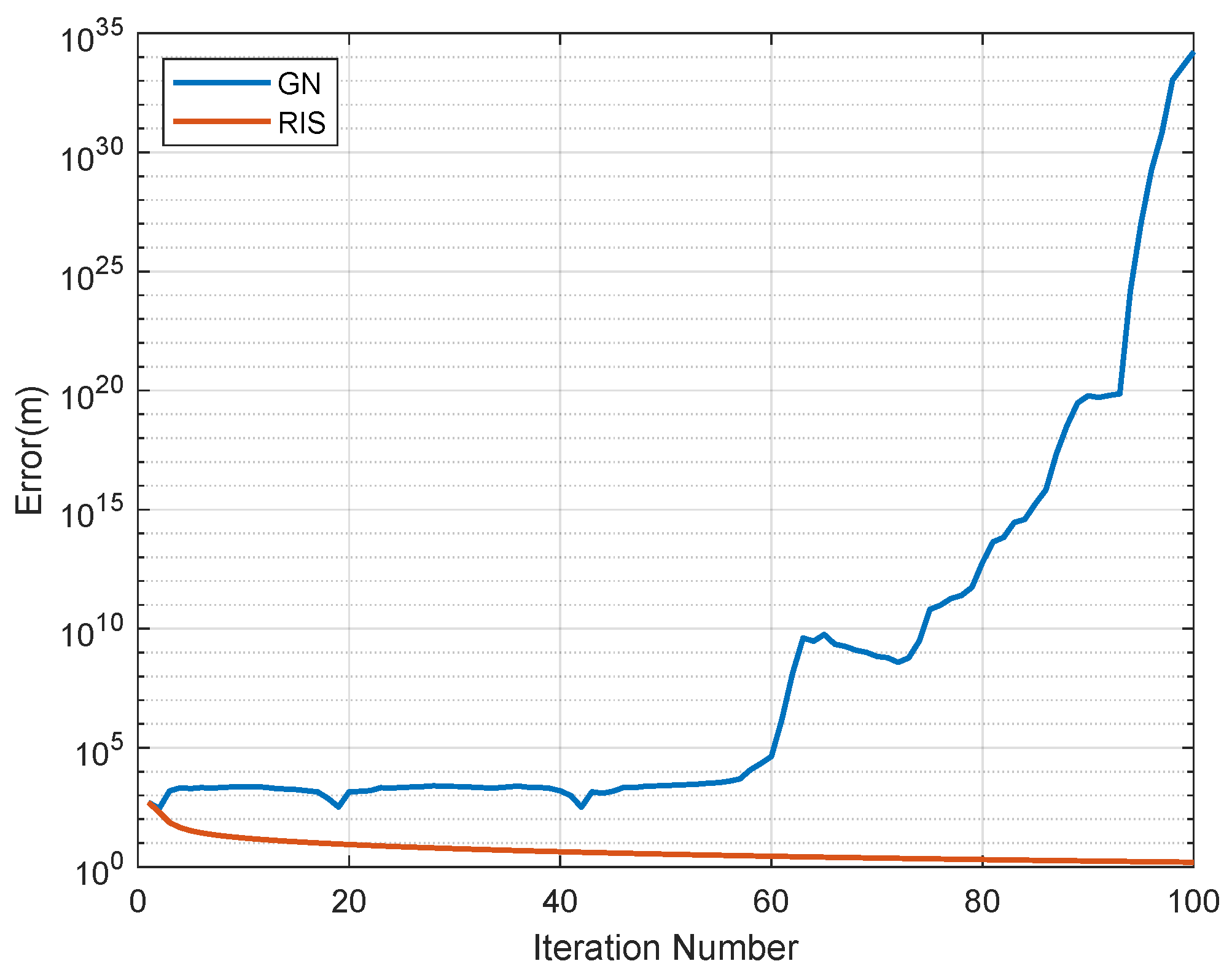
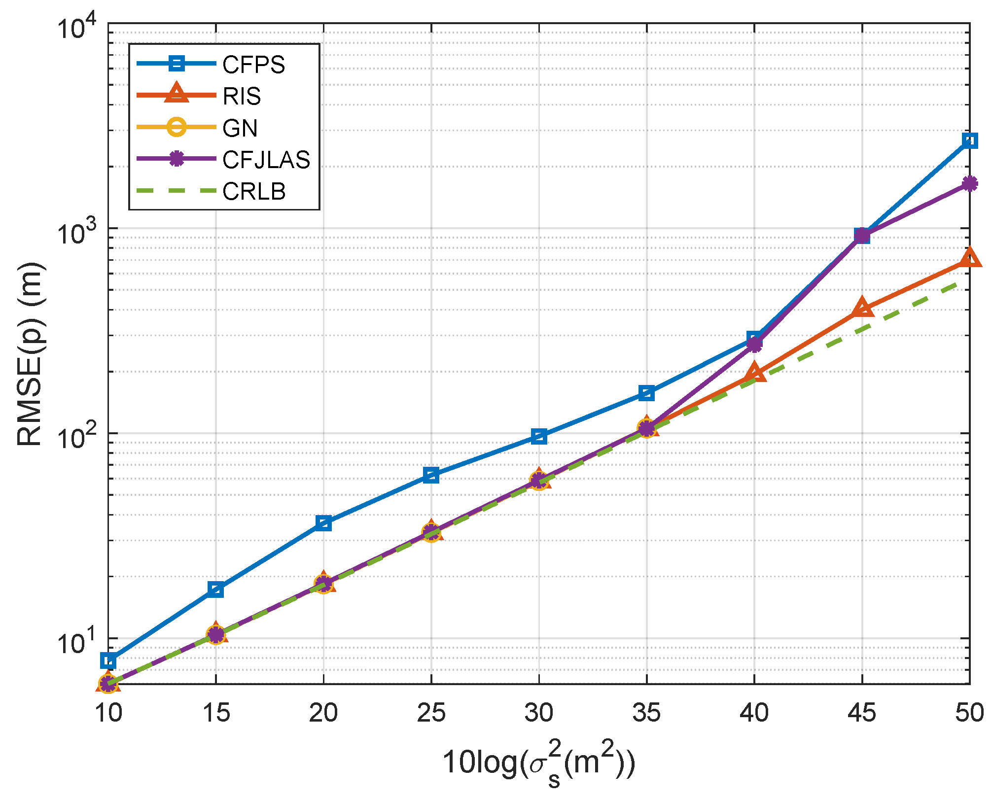
• A robust iteration solution based on factor graphs and message passing, resilient to noise and AN position error, ensuring global convergence.
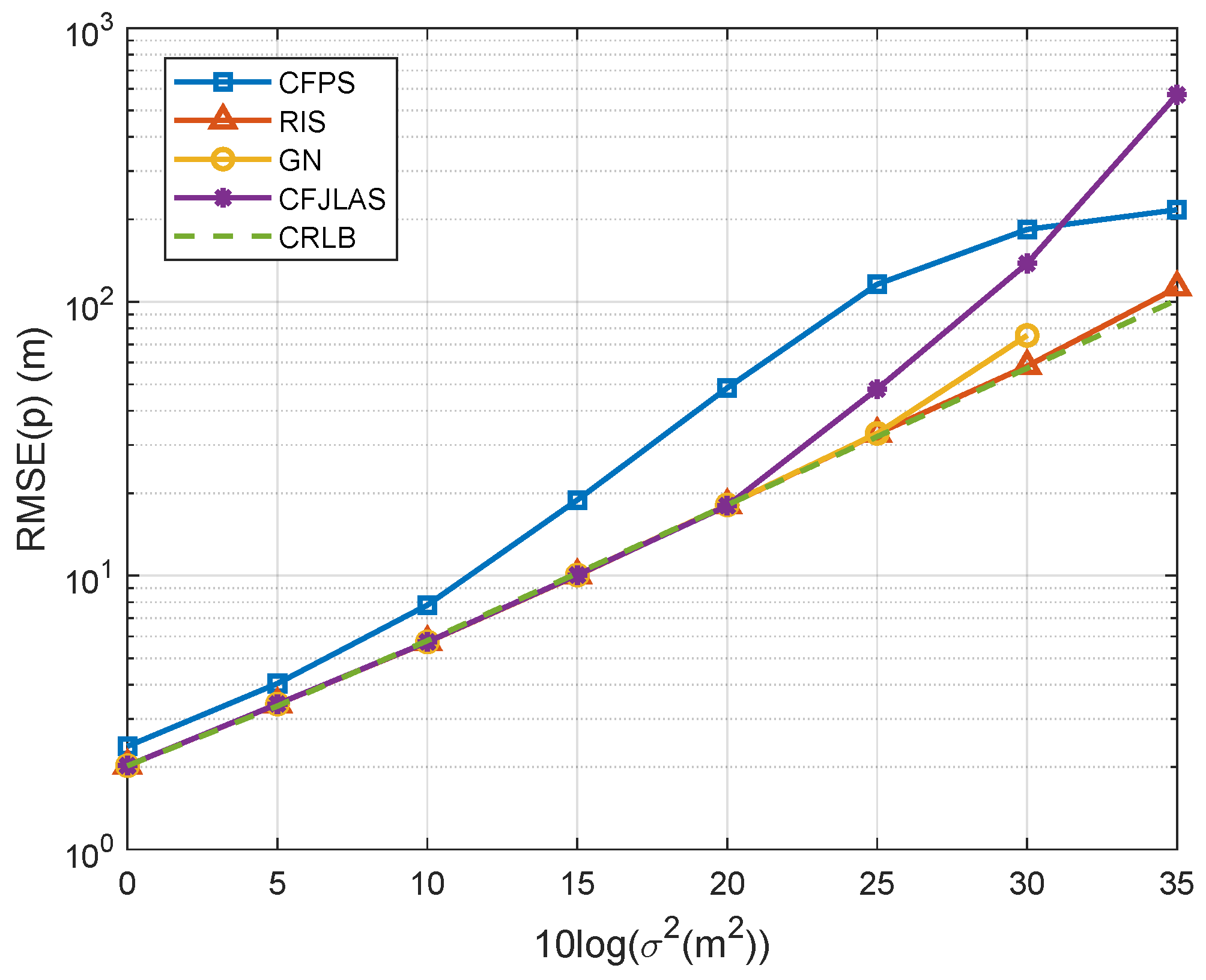
• Theoretical analysis corroborating the optimality in the RMSE of the proposed RIS.
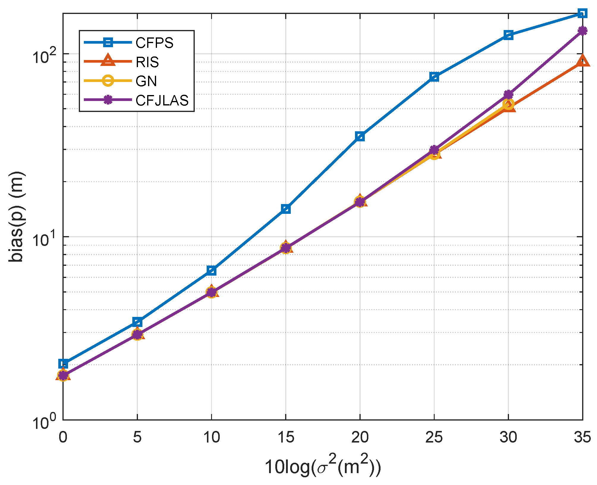
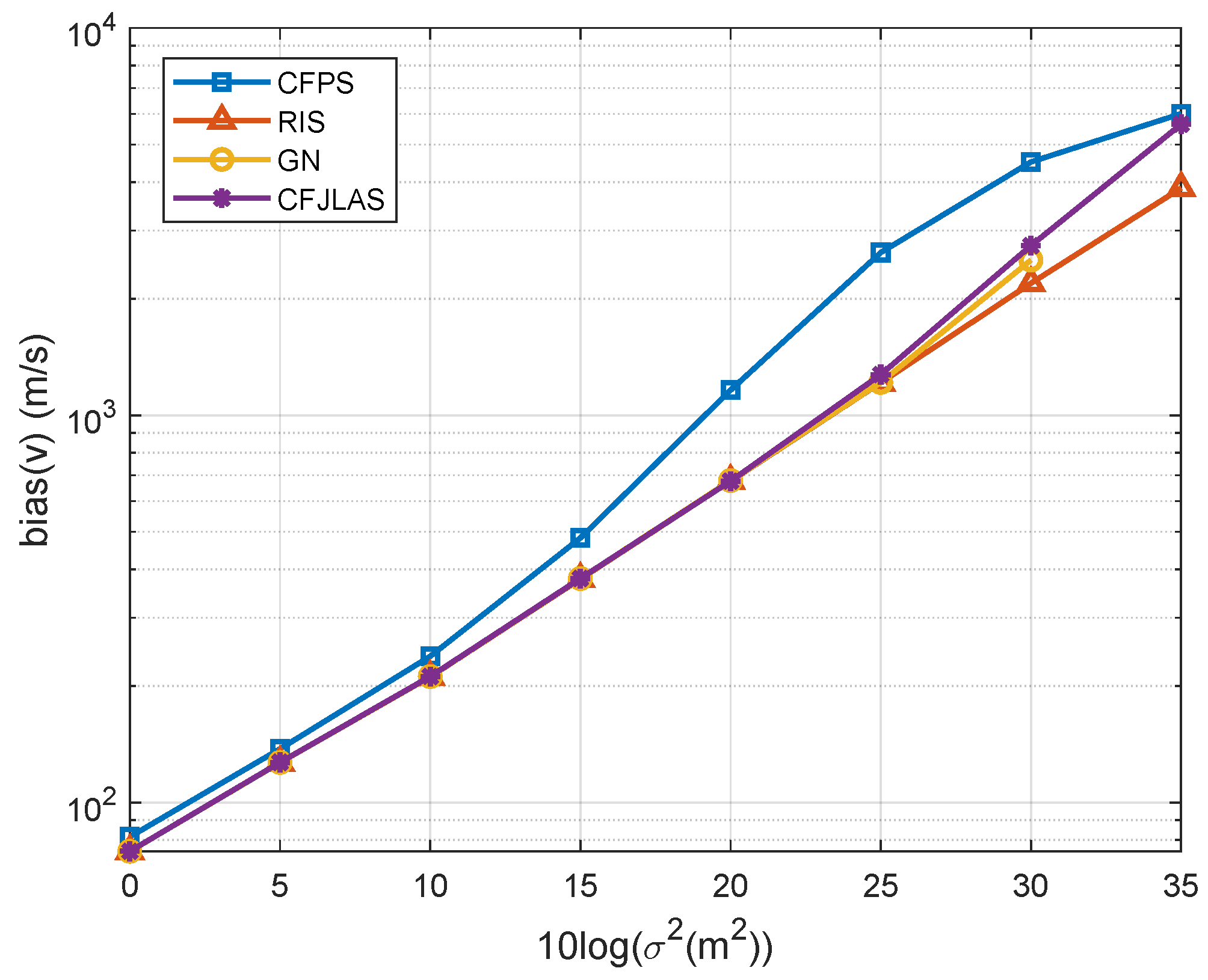
• Extensive simulations validating the analytical results, demonstrating the best bias performance, and confirming the manageable computational complexity.

The remaining sections of this paper are structured as follows. Section 2 elucidates the measurement model and formulates the JLAS problem based on sequential TOA for mobile UNs. Section 3 presents the proposed method that firstly solves the JLAS problem using two-stage weighted least squares, followed by a novel robust iteration. The CRLB and theoretical analysis are performed in Section 4. Section 5 presents the simulation experiments conducted to assess the performance of the proposed method. The summary and future research of this paper are concluded in Section 6.

To enhance readability, this paper uses bold uppercase letters and symbols to represent matrices and bold lowercase for vectors. $\parallel ·\parallel$, ^⊤, and ${ }^{-1}$ are the Euclidean norm, transpose, and inverse operators. $x\left(i\right)$ is the i-th element of $\mathbf{x}$. $\mathbf{x}(i:j)$ denotes a subvector constructed by the i-th to j-th elements of $\mathbf{x}$. $\mathbf{X}(:,i)$ means the i-th column of matrix $\mathbf{X}$. Notations with a superscript ${·}^o$ denote true values. Letters and symbols with a hat $\widehat{·}$ represent the estimate values, while those without any superscript signify measured values. The notations used in this paper are listed at the end of this paper.

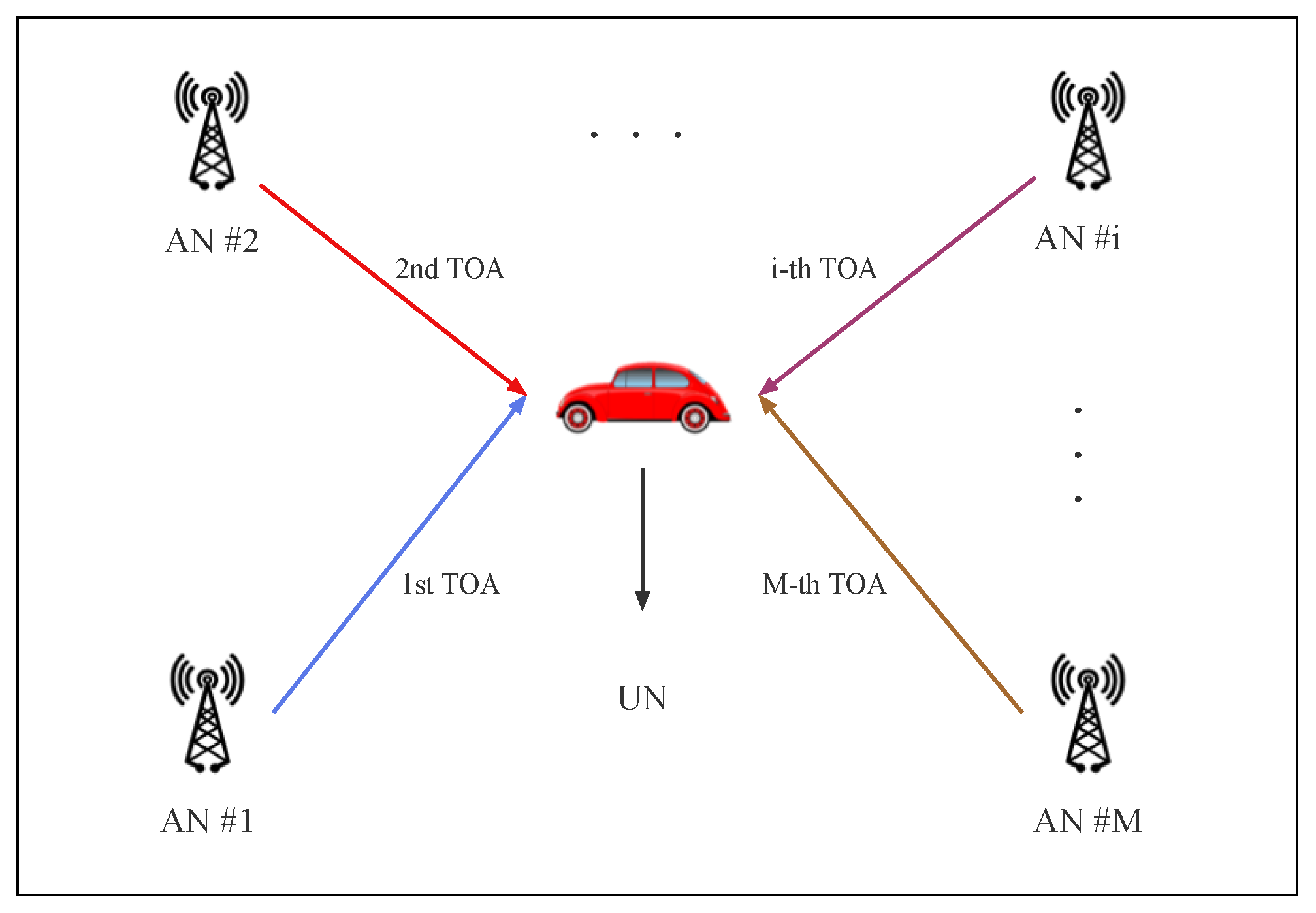
2. One-Way TOA Measurement Model

The WSN consists of M ANs and one mobile UN in a N-dimensional space, where $N=2\mathrm{or}3$, as depicted in Figure 1. The true position of AN $\#i$ is ${\mathbf{s}}_i^o$, $i=1,2,\cdots ,M$, which is static. ANs are synchronized so the clock offset ${\upsilon }_i$, $i=1,2,\cdots ,M$, among the ANs that are known. As discussed in the Introduction, the system considered in this paper employs a TD broadcasting at ANs that transmit packets in a synchronized and pre-arranged sequential order. The UN passively receives these packets to obtain sequential TOA measurements, enabling JLAS. Since the transmission is one-way from the ANs to the UN, only one-way TOA measurements are available to the UN. The position and velocity of the mobile UN are unknown, denoted by ${\mathbf{p}}^o$ and ${\mathbf{v}}^o$. Assume that the velocity is constant within a TD broadcasting cycle. Since the clock of the UN is not synchronized to that of the ANs, the clock offset and clock skew are unknown. The one-way TOA from AN $\#i$ to the UN is

$${\tau }_i^o=\frac{\parallel {\mathbf{p}}^o+{\mathbf{v}}^o{t}_i-{\mathbf{s}}_i^o\parallel }{c}+{\tau }_{off}^o+{\tau }_{dft}^o{t}_i-{\upsilon }_i,$$

(1)

where $t_i$ represents the known time interval between the start time of the TD broadcasting cycle and AN $\#i$’s launch time, c is the light speed, ${\tau }_{off}^o$ is the clock offset, ${\tau }_{dft}^o$ is the clock skew, and ${\upsilon }_i$ is the clock offset of AN $\#i$. In assuming that c is a known constant for the WSN, the TOA is interchangeable with the range-of-arrival:

$$r_i^o=\parallel {\mathbf{p}}^o+{\mathbf{v}}^o{t}_i-{\mathbf{s}}_i^o\parallel +{\gamma }^o+{\iota }^o{t}_i-{\gamma }_i,$$

(2)

where $r_i^o=c{\tau }_i^o$, ${\gamma }^o=c{\tau }_{off}^o$, ${\iota }^o=c{\tau }_{dft}^o$, ${\gamma }_i=c{\upsilon }_i$, and ${\gamma }^o$ and ${\iota }^o$ are the distance form of the clock offset and clock skew. So, the measured TOA is

$$r_i=r_i^o+{\epsilon }_i,i=1,\cdots ,M,$$

(3)

where ${\epsilon }_i$ represents the measurement noise, following an independent zero-mean Gaussian distribution with a variance of ${\sigma }_i^2$, i.e., ${\epsilon }_i\sim \mathcal{N}(0,{\sigma }_i^2)$. The measurements from all ANs are

$$\mathbf{r}={\mathbf{r}}^o+\mathit{\epsilon },$$

(4)

where $\mathbf{r}={[r_1,r_2,\cdots ,r_M]}^T$, ${\mathbf{r}}^o={[r_1^o,r_2^o,\cdots ,r_M^o]}^T$, and $\mathit{\epsilon }={[{\epsilon }_1,{\epsilon }_2,\cdots ,{\epsilon }_M]}^T$. The covariance matrix of $\mathit{\epsilon }$ is ${\mathbf{Q}}_{\epsilon }=E\left[\mathit{\epsilon }{\mathit{\epsilon }}^T\right]$.

Typically, the true position of AN $\#i$ is not known, which is usually obtained through measurement or estimation; hence, it may contain an error represented by $\Delta {\mathbf{s}}_i$. The erroneous position of AN $\#i$ is

$${\mathbf{s}}_i={\mathbf{s}}_i^o-\Delta {\mathbf{s}}_i,i=1,\cdots ,M.$$

(5)

where the error $\Delta {\mathbf{s}}_i$ follows a zero-mean Gaussian distribution, $\Delta {\mathbf{s}}_i\sim \mathcal{N}(0,{\sigma }_{{\mathbf{s}}_i}^2)$. In collecting all position errors in vector form, $\Delta \mathbf{s}={[\Delta {\mathbf{s}}_1^T,\Delta {\mathbf{s}}_2^T,\cdots ,\Delta {\mathbf{s}}_M^T]}^T$, the covariance matrix of position errors is ${\mathbf{Q}}_s=E[\Delta \mathbf{s}\Delta {\mathbf{s}}^T]$.

The goal of this study was to assess the position, velocity, and clock parameters of a mobile UN using sequential TOA measurements provided in (3) when the positions of the ANs are not accurately known, improving the robustness to noise and error with manageable complexity.

3. Proposed Solutions

3.1. Problem Formulation

The measurement model given in (4) is nonlinear. We shall first formulate an optimization problem related to the unknown UN position, velocity, clock offset, and clock drift.

Let us start with (2). Keeping the norm on the right side, moving the rest of the terms to the left, and substituting (3) yield

$$\begin{array}{c}\hfill r_i+{\gamma }_i-{\gamma }^o-{\iota }^o{t}_i-{\epsilon }_i=\parallel {\mathbf{p}}^o+{\mathbf{v}}^o{t}_i-{\mathbf{s}}_i-\Delta {\mathbf{s}}_i\parallel ,i=1,\cdots M.\end{array}$$

(6)

Squaring both sides of (6) above and using the mathematical truth ${\parallel \mathbf{x}\parallel }^2={\mathbf{x}}^T\mathbf{x}$, we have

$$\begin{array}{cc}\hfill & \parallel {\mathbf{s}}_i{\parallel }^2-{\alpha }_i^2-t_i^2({\iota }^{o2}-\parallel {\mathbf{v}}^o{\parallel }^2)-2{\mathbf{s}}_i^T{\mathbf{p}}^o-2t_i{\mathbf{s}}_i^T{\mathbf{v}}^o+2{\alpha }_i{\gamma }^o+2t_i{\alpha }_i{\iota }^o\hfill \\ \hfill & -2t_i({\gamma }^o{\iota }^o-{\mathbf{p}}^{oT}{\mathbf{v}}^o)-({\gamma }^{o2}-\parallel {\mathbf{p}}^o{\parallel }^2)={\varrho }_i+{\epsilon }_i^2-2\Delta {\mathbf{s}}_i^T\Delta {\mathbf{s}}_i,i=1,\cdots M,\hfill \end{array}$$

(7)

where ${\alpha }_i=r_i+{\gamma }_i$, and the first-order noise and error term ${\varrho }_i=-2({\alpha }_i-{\gamma }^o-{\iota }^o{t}_i){\epsilon }_i+2({\mathbf{p}}^{oT}+t_i{\mathbf{v}}^{oT}-{\mathbf{s}}_i^{oT})\Delta {\mathbf{s}}_i.$

To remove the term ${\gamma }^{o2}-{\parallel {\mathbf{p}}^o\parallel }^2$, we can subtract (7) with that with a fixed i. Without loss of generality, we choose the subtracted equation with subscript $i=1$ and obtain

$$\begin{array}{cc}\hfill & \parallel {\mathbf{s}}_1{\parallel }^2-{\alpha }_1^2-t_1^2({\iota }^{o2}-\parallel {\mathbf{v}}^o{\parallel }^2)-2{\mathbf{s}}_1^T{\mathbf{p}}^o-2t_1{\mathbf{s}}_1^T{\mathbf{v}}^o+2{\alpha }_1{\gamma }^o+2t_1{\alpha }_1{\iota }^o\hfill \\ \hfill & -2t_1({\gamma }^o{\iota }^o-{\mathbf{p}}^{oT}{\mathbf{v}}^o)-({\gamma }^{o2}-\parallel {\mathbf{p}}^o{\parallel }^2)={\varrho }_1+{\epsilon }_1^2-2\Delta {\mathbf{s}}_1^T\Delta {\mathbf{s}}_1.\hfill \end{array}$$

(8)

Subtracting (8) from (7) and ignoring the noise and error terms higher than the first order yield

$$\begin{array}{cc}\hfill & \parallel {\mathbf{s}}_i{\parallel }^2-{\parallel {\mathbf{s}}_1\parallel }^2-({\alpha }_i^2-{\alpha }_1^2)-2({\mathbf{s}}_i^T-{\mathbf{s}}_1^T){\mathbf{p}}^o-2(t_i{\mathbf{s}}_i^{oT}-t_1{\mathbf{s}}_1^{oT}){\mathbf{v}}^o-2({\alpha }_1-{\alpha }_i){\gamma }^o\hfill \\ \hfill & -2(t_1{\alpha }_1-t_i{\alpha }_i){\iota }^o+(t_1^2-t_i^2)({\iota }^{o2}-\parallel {\mathbf{v}}^o{\parallel }^2)+2(t_1-t_i)({\gamma }^o{\iota }^o-{\mathbf{p}}^{oT}{\mathbf{v}}^o)\hfill \\ \hfill & ={\varrho }_i-{\varrho }_1,i=2,\cdots ,M.\hfill \end{array}$$

(9)

The equation above is a pseudolinear equation associated with ${\mathbf{p}}^o$, ${\mathbf{v}}^o$, ${\gamma }^o$, and ${\iota }^o$. Let the unknown parameters be ${\mathit{\varphi }}^o$ = $[{\mathbf{p}}^{oT},{\mathbf{v}}^{oT},{\gamma }^o,{\iota }^o,{\iota }^{o2}-\parallel {\mathbf{v}}^o{{\parallel }^2,{\gamma }^o{\iota }^o-{\mathbf{p}}^{oT}{\mathbf{v}}^o]}^T$, and (9) can be collected in matrix form. We have

$$\mathbf{h}-\mathbf{G}{\mathit{\varphi }}^o=\mathbf{B}\mathit{\epsilon }+\mathbf{C}\Delta \mathbf{s},$$

(10)

where

$$\begin{array}{cc}\hfill \mathbf{h}& =\left[\begin{array}{c}\parallel {\mathbf{s}}_2{\parallel }^2-{\parallel {\mathbf{s}}_1\parallel }^2-({\alpha }_2^2-{\alpha }_1^2)\\ ⋮\\ \parallel {\mathbf{s}}_M{\parallel }^2-{\parallel {\mathbf{s}}_1\parallel }^2-({\alpha }_M^2-{\alpha }_1^2)\end{array}\right],\hfill \end{array}$$

(11)

$$\begin{array}{cc}\hfill \mathbf{G}(:,1:2N+1)& =\left[\begin{array}{ccc}2{({\mathbf{s}}_2-{\mathbf{s}}_1)}^T& 2{(t_2{\mathbf{s}}_2-t_1{\mathbf{s}}_1)}^T& 2({\alpha }_1-{\alpha }_2)\\ ⋮& ⋮& ⋮\\ 2{({\mathbf{s}}_M-{\mathbf{s}}_1)}^T& 2{(t_M{\mathbf{s}}_M-t_1{\mathbf{s}}_1)}^T& 2({\alpha }_1-{\alpha }_M)\end{array}\right],\hfill \\ \hfill \end{array}$$

(12)

$$\begin{array}{cc}\hfill \mathbf{G}(:,2N+2:2N+4)& =\left[\begin{array}{ccc}2(t_1{\alpha }_1-t_2{\alpha }_2)& -(t_1^2-t_2^2)& -2(t_1-t_2)\\ ⋮& ⋮& ⋮\\ 2(t_1{\alpha }_1-t_M{\alpha }_M)& -(t_1^2-t_M^2)& -2(t_1-t_M)\end{array}\right],\hfill \end{array}$$

(13)

$$\begin{array}{cc}\hfill \mathbf{B}& =\left[\begin{array}{cccc}2({\alpha }_1-{\gamma }^o-{\iota }^o{t}_1)& -2({\alpha }_2-{\gamma }^o-{\iota }^o{t}_2)& \cdots & 0\\ ⋮& ⋮& \ddots & ⋮\\ 2({\alpha }_1-{\gamma }^o-{\iota }^o{t}_1)& 0& \cdots & -2({\alpha }_M-{\gamma }^o-{\iota }^o{t}_M)\end{array}\right],\hfill \end{array}$$

(14)

and

$$\begin{array}{cc}\hfill \mathbf{C}& =\left[\begin{array}{cccc}-2{({\mathbf{p}}^o+t_1{\mathbf{v}}^o-{\mathbf{s}}_1)}^T& 2{({\mathbf{p}}^o+t_2{\mathbf{v}}^o-{\mathbf{s}}_2)}^T& \cdots & {\mathbf{0}}_N^T\\ ⋮& ⋮& \ddots & ⋮\\ -2{({\mathbf{p}}^o+t_1{\mathbf{v}}^o-{\mathbf{s}}_1)}^T& {\mathbf{0}}_N& \cdots & 2{({\mathbf{p}}^o+t_M{\mathbf{v}}^o-{\mathbf{s}}_M)}^T\end{array}\right].\hfill \end{array}$$

(15)

Finding the estimation of ${\mathbf{p}}^o$, ${\mathbf{v}}^o$, ${\gamma }^o$, and ${\iota }^o$ can be formulated as an optimization problem:

$$\begin{array}{cc}\hfill & \underset{\mathbf{p},\mathbf{v},\gamma ,\iota }{min}{(\mathbf{h}-\mathbf{G}\mathit{\varphi })}^T\mathbf{W}(\mathbf{h}-\mathbf{G}\mathit{\varphi })\hfill \end{array}$$

(16)

$$\begin{array}{cc}\hfill & \mathrm{s}.\mathrm{t}.\varphi (2N+3)=\varphi {(2N+2)}^2-{\parallel \mathit{\varphi }(N+1:2N)\parallel }^2,\hfill \end{array}$$

(17)

$$\begin{array}{cc}\hfill & \varphi (2N+4)=\varphi (2N+1)\varphi (2N+2)-\mathit{\varphi }{(1:N)}^T\mathit{\varphi }(N+1:2N),\hfill \end{array}$$

(18)

where

$$\begin{array}{c}\hfill \mathbf{W}={(\mathbf{B}{\mathbf{Q}}_{\epsilon }{\mathbf{B}}^T+\mathbf{C}{\mathbf{Q}}_s{\mathbf{C}}^T)}^{-1}.\end{array}$$

(19)

3.2. Closed-Form Solution by Nullspace Projection

The optimization problem (16)–(18) is nonconvex and cannot be solved straightforwardly. The pseudo-linearization introduces two redundant variables. We shall first eliminate them from ${\mathit{\varphi }}^o$ to reduce the dimension of unknowns, and solve ${\mathbf{p}}^o$, ${\mathbf{v}}^o$, ${\gamma }^o$, and ${\iota }^o$ in two stages. In partitioning ${\mathit{\varphi }}^o$ into two parts ${\mathit{\varphi }}^o={[{\mathit{\mu }}^{oT},{\mathbf{\nu }}^{oT}]}^T$, where

$$\begin{array}{cc}\hfill {\mathit{\mu }}^o& ={\mathit{\varphi }}^o(1:2N+2),\hfill \end{array}$$

(20)

$$\begin{array}{cc}\hfill {\mathbf{\nu }}^o& ={\mathit{\varphi }}^o(2N+3:2N+4).\hfill \end{array}$$

(21)

${\mathbf{\nu }}^o$ contains the redundant variables only. Thus, (10) can be reformulated as

$$\mathbf{h}-{\mathbf{G}}_3{\mathit{\mu }}^o-{\mathbf{G}}_4{\mathbf{\nu }}^o=\mathbf{B}\mathit{\epsilon }+\mathbf{C}\Delta \mathbf{s},$$

(22)

where ${\mathbf{G}}_3=\mathbf{G}(:,1:2N+2)$, and ${\mathbf{G}}_4=\mathbf{G}(:,2N+3:2N+4)$.

In order to eliminate the term related to ${\mathbf{\nu }}^o$, we shall project the equation above to the nullspace of ${\mathbf{G}}_4$. Let $\mathbf{V}$ be the matrix consisting of the columns from an orthonormal basis of ${\mathbf{G}}_4^T$, satisfying

$${\mathbf{V}}^T{\mathbf{G}}_4=\mathbf{O}.$$

(23)

We shall note that $\mathbf{V}$ is not unique, since pre-multiplying any appropriately sized matrix on $\mathbf{V}$ can guarantee the relationship in (23). A selection of $\mathbf{V}$ is from any $M-3$ columns from the orthogonal projection matrix of ${\mathbf{G}}_4$, ${\mathbf{G}}_4^{\perp }=\mathbf{I}-{\mathbf{G}}_4{\left({\mathbf{G}}_4^T{\mathbf{G}}_4\right)}^{-1}{\mathbf{G}}_4^T$. Pre-multiplying (22) by ${\mathbf{V}}^T$ yields

$${\mathbf{z}}_1-{\mathbf{A}}_1{\mathit{\mu }}^o=\mathbf{D}\mathit{\epsilon }+\mathbf{F}\Delta \mathbf{s},$$

(24)

where

$$\begin{array}{c}\hfill {\mathbf{z}}_1={\mathbf{V}}^T\mathbf{h},{\mathbf{A}}_1={\mathbf{V}}^T{\mathbf{G}}_3,\mathbf{D}={\mathbf{V}}^T\mathbf{B},\mathbf{F}={\mathbf{V}}^T\mathbf{C}.\end{array}$$

(25)

The estimation of ${\mathit{\mu }}^o$ in terms of WLS is

$$\widehat{\mathit{\mu }}={\left({\mathbf{A}}_1^T{\mathbf{W}}_1{\mathbf{A}}_1\right)}^{-1}{\mathbf{A}}_1^T{\mathbf{W}}_1{\mathbf{z}}_1,$$

(26)

where

$$\begin{array}{c}\hfill {\mathbf{W}}_1={(\mathbf{D}{\mathbf{Q}}_{\epsilon }{\mathbf{D}}^T+\mathbf{F}{\mathbf{Q}}_s{\mathbf{F}}^T)}^{-1}.\end{array}$$

(27)

Projecting (22) to the nullspace of ${\mathbf{G}}_4$ ignores the constraints among the eliminated variables and the interested unknowns; thus, the WLS solution above is suboptimal. We now leverage the constraints to improve the coarse solution above. Denoting the errors in (26) as $\Delta \mathit{\mu }$, $\Delta \mathbf{p}$, $\Delta \mathbf{v}$, $\Delta \gamma$, and $\Delta \iota$, respectively, we have

$$\begin{array}{cc}\hfill {\mathbf{p}}^o& =\mathbf{p}-\Delta \mathbf{p},\hfill \end{array}$$

(28)

$$\begin{array}{cc}\hfill {\mathbf{v}}^o& =\mathbf{v}-\Delta \mathbf{v},\hfill \end{array}$$

(29)

$$\begin{array}{cc}\hfill {\gamma }^o& =\gamma -\Delta \gamma ,\hfill \end{array}$$

(30)

$$\begin{array}{cc}\hfill {\iota }^o& =\iota -\Delta \iota ,\hfill \end{array}$$

(31)

where $\mathbf{p}=\widehat{\mathit{\mu }}(1:N)$, $\mathbf{v}=\widehat{\mathit{\mu }}(N+1:2N)$, $\gamma =\widehat{\mu }(2N+1)$, and $\iota =\widehat{\mu }(2N+2)$. Substituting (28)–(31) with the last to elements of ${\mathit{\varphi }}^o$ and neglecting the second-order error terms yield

$$\begin{array}{cc}\hfill {\iota }^{o2}-{\parallel {\mathbf{v}}^o\parallel }^2& ={(\iota -\Delta \iota )}^2-{(\mathbf{v}-\Delta \mathbf{v})}^T(\mathbf{v}-\Delta \mathbf{v})\hfill \end{array}$$

$$\approx {\iota }^2-{\parallel \mathbf{v}\parallel }^2+2{\mathbf{v}}^T\Delta \mathbf{v}-2\iota \Delta \iota ,$$

(32)

$${\gamma }^o{\iota }^o-{\mathbf{p}}^{oT}{\mathbf{v}}^o=(\gamma -\Delta \gamma )(\iota -\Delta \iota )-{(\mathbf{p}-\Delta \mathbf{p})}^T(\mathbf{v}-\Delta \mathbf{v})$$

$$\begin{array}{cc}\hfill & \approx \gamma \iota -{\mathbf{p}}^T\mathbf{v}+{\mathbf{v}}^T\Delta \mathbf{p}+{\mathbf{p}}^T\Delta \mathbf{v}-\iota \Delta \gamma -\gamma \Delta \iota .\hfill \end{array}$$

(33)

Substituting (28)–(33) into ${\mathit{\varphi }}^o$ and organizing it into matrix form give

$${\mathit{\varphi }}^o=\mathit{\varphi }-\mathbf{H}\Delta \mathit{\mu },$$

(34)

where

$$\begin{array}{c}\hfill \mathit{\varphi }=\left[\begin{array}{c}\mathbf{p}\\ \mathbf{v}\\ \gamma \\ \iota \\ {\iota }^2-{\parallel \mathbf{v}\parallel }^2\\ \gamma \iota -{\mathbf{p}}^T\mathbf{v}\end{array}\right],\mathbf{H}=\left[\begin{array}{cccc}{\mathbf{I}}_N& {\mathbf{O}}_N& 0& 0\\ {\mathbf{O}}_N& {\mathbf{I}}_N& 0& 0\\ {\mathbf{O}}_N& {\mathbf{O}}_N& 1& 0\\ {\mathbf{O}}_N& {\mathbf{O}}_N& 0& 1\\ {\mathbf{O}}_N& -2{\mathbf{v}}^T& 0& 2\iota \\ -{\mathbf{v}}^T& {\mathbf{p}}^T& \iota & \gamma \end{array}\right],\Delta \mathit{\mu }=\left[\begin{array}{c}\Delta \mathbf{p}\\ \Delta \mathbf{v}\\ \Delta \gamma \\ \Delta \iota \end{array}\right].\end{array}$$

(35)

Inserting (34) into (10) gives a new equation with respect to the estimation errors:

$$\mathbf{h}-\mathbf{G}\mathit{\varphi }+\mathbf{GH}\Delta \mathit{\mu }=\mathbf{B}\mathit{\epsilon }+\mathbf{C}\Delta \mathbf{s},$$

(36)

Similarly, the estimation of $\Delta \mathit{\mu }$ can be obtained through the WLS as

$$\Delta \widehat{\mathit{\mu }}=-{\left({\mathbf{H}}^T{\mathbf{G}}^T{\mathbf{W}}_2\mathbf{G}\mathbf{H}\right)}^{-1}{\mathbf{H}}^T{\mathbf{G}}^T{\mathbf{W}}_2(\mathbf{h}-\mathbf{G}\mathit{\varphi })$$

(37)

where the weighting matrix

$$\begin{array}{c}\hfill {\mathbf{W}}_2={(\mathbf{B}{\mathbf{Q}}_{\epsilon }{\mathbf{B}}^T+\mathbf{C}{\mathbf{Q}}_s{\mathbf{C}}^T)}^{-1}.\end{array}$$

(38)

Finally, subtracting the estimated error $\Delta \widehat{\mathit{\mu }}$ from $\widehat{\mathit{\mu }}$, we obtain a better solution:

$$\check{\mathit{\mu }}=\widehat{\mathit{\mu }}-\Delta \widehat{\mathit{\mu }}.$$

(39)

The weighting matrices ${\mathbf{W}}_1$ and ${\mathbf{W}}_2$ depend on unknown parameters to be estimated. We shall set them as identity matrices to generate a pre-estimation, which will be put back to update ${\mathbf{W}}_1$ and ${\mathbf{W}}_2$ to obtain a better result. Repeating this one or two times is sufficient for an accurate solution, as the estimation is not very sensitive to the weighting matrices [28,29,30].

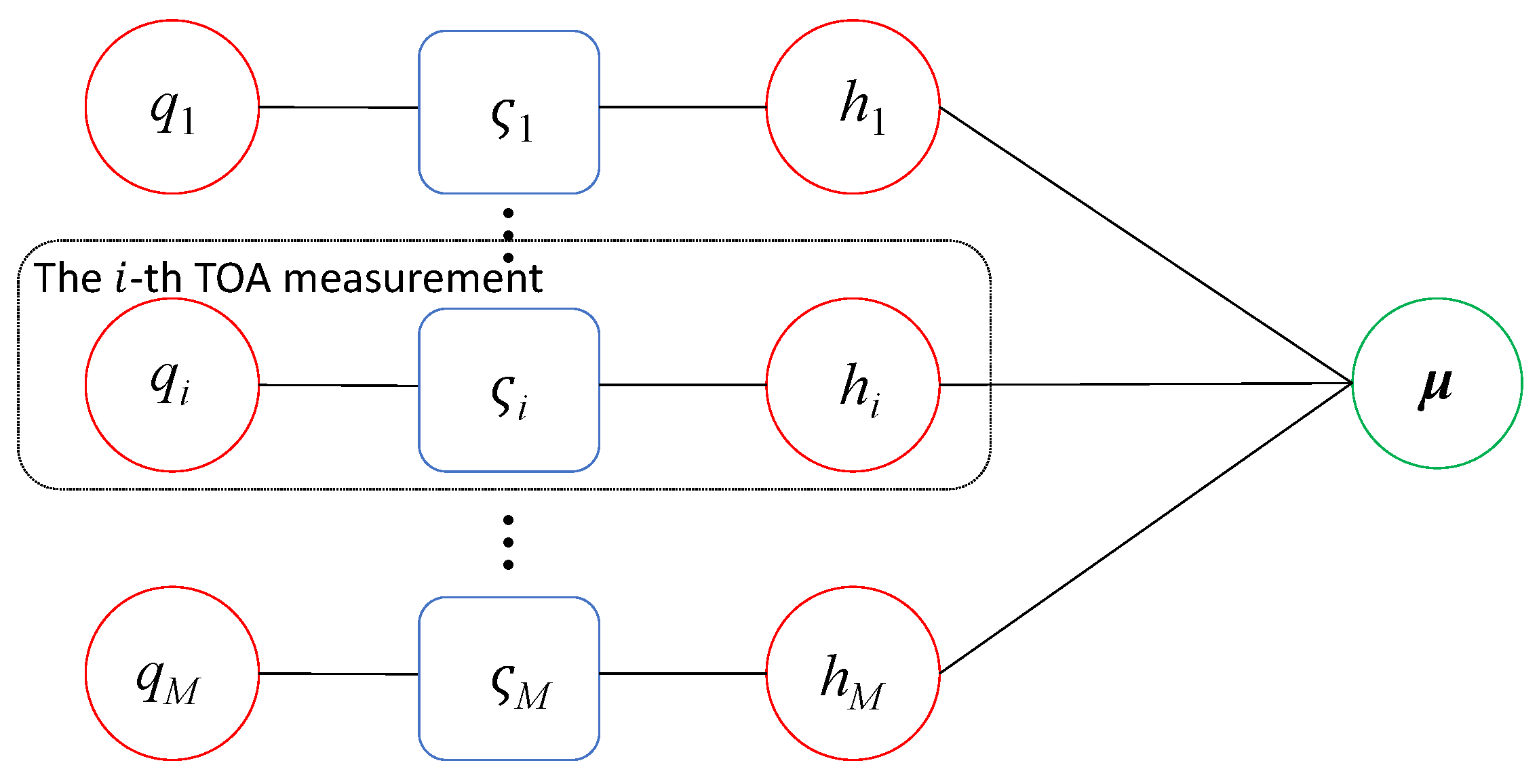
3.3. Robust Iterative Solution

The solution above is not optimal, due to the optimization problem (16)–(18) not considering the inner relationship between the last two elements of ${\mathit{\varphi }}^o$; thus, the result cannot attain the CRLB, as shown in Section 5. Ref. [11] formulated the same optimization problem and solved it using a constrained WLS (CWLS), but the CWLS does not reach the CRLB either. Ref. [11] applied Taylor expansion to formulate a new problem that refines the accuracy. Although the final solution has an appropriate mean square error (MSE) for the CRLB level when the noise is small, it is not sufficiently robust to noise and deviates from the CRLB if the noise is relatively large. Factor graphing (FG) has been applied to the complex localization problem [31,32,33]. Once the problem is formulated through factor graphs, finding an effective solution using the sum-product algorithm (SPA) operated by message passing is trivial. FG can provide an iteration solution resilient to noise and initialization [34], which is feasible to the sequential TOA JLAS problem. FG can converge to the optimal, notwithstanding the estimator in Section 3.2 being suboptimal.

Factor graphs of sequential TOA JLAS are shown in Figure 2. The rounded rectangles represent the factor nodes, and the circles are variable nodes. Edges connect factor nodes, and variable nodes are the arguments of a local function. Let us start from the maximum likelihood (ML) cost function:

$$\begin{array}{c}\hfill \mathcal{J}\left(\mathit{\mu }\right)=exp\left\{{(\mathbf{r}-\overline{\mathbf{r}}\left(\mathit{\mu }\right))}^T\mathcal{W}(\mathbf{r}-\overline{\mathbf{r}}\left(\mathit{\mu }\right))\right\},\end{array}$$

(40)

where

$$\begin{array}{c}\hfill {\mathcal{W}}^{-1}={\mathbf{Q}}_{\epsilon }+\left(\frac{\partial {\mathbf{r}}^o}{\partial {\mathbf{s}}^{oT}}{\mathbf{Q}}_s\frac{\partial {\mathbf{r}}^{oT}}{\partial {\mathbf{s}}^o}\right).\end{array}$$

(41)

In assuming that $\mathcal{W}$ is diagonal, although it is commonly not, the conclusion does not affect this assumption. ML cost (40) can be rewritten as

$$\begin{array}{c}\hfill \mathcal{J}\left(\mathit{\mu }\right)=\prod _{i=1}^{M}exp\left\{w_i{(r_i-{\overline{r}}_i\left(\mathit{\mu }\right))}^2\right\},\end{array}$$

(42)

where $w_i$ is the i-$th$ diagonal element of $\mathcal{W}$. Denote

$$\begin{array}{cc}\hfill h_i({\varsigma }_i,\mathit{\mu })& =\delta ({\varsigma }_i-{\overline{r}}_i\left(\mathit{\mu }\right)),\hfill \end{array}$$

(43)

$$\begin{array}{cc}\hfill q_i\left({\varsigma }_i\right)& =exp\left\{w_i{(r_i-{\varsigma }_i)}^2\right\},\hfill \end{array}$$

(44)

where $\delta (·)$ is the Dirac delta function. Figure 2 indicates that the marginal or belief of $\mathit{\mu }$ is the product of all M incoming messages:

$$\begin{array}{c}\hfill \mathcal{B}\left(\mathit{\mu }\right)=\prod _{i=1}^M{\varpi }_{h_i\to \mathit{\mu }}\left(\mathit{\mu }\right).\end{array}$$

(45)

Since the noise and errors are assumed to be Gaussian, the message from node $q_i$ to ${\varsigma }_i$ is

$$\begin{array}{c}\hfill {\varpi }_{q_i\to {\varsigma }_i}\left({\varsigma }_i\right)\sim \mathcal{N}(\varsigma ;r_i,w_i).\end{array}$$

(46)

The message ${\varpi }_{q_i\to {\varsigma }_i}\left({\varsigma }_i\right)$ is forwarded to the function node $h_i$ by

$$\begin{array}{c}\hfill {\varpi }_{{\varsigma }_i\to h_i}\left({\varsigma }_i\right)={\varpi }_{q_i\to {\varsigma }_i}\left({\varsigma }_i\right),\end{array}$$

(47)

which follows a Gaussian distribution. In applying the SPA, the outgoing message from the factor node $h_i$ to the variable node $\mathit{\mu }$ is the integration of the product of $h_i$ and all incoming messages to $h_i$ over the variable ${\varsigma }_i$:

$$\begin{array}{c}\hfill {\varpi }_{h_i\to \mathit{\mu }}\left(\mathit{\mu }\right)=\int h_i({\varsigma }_i,\mathit{\mu }){\varpi }_{{\varsigma }_i\to h_i}\left({\varsigma }_i\right)d{\varsigma }_i.\end{array}$$

(48)

Expanding ${\overline{r}}_i\left(\mathit{\mu }\right)$ in $h_i({\varsigma }_i,\mathit{\mu })$ by the first-order Taylor series at the estimate $\check{\mathit{\mu }}$ results in

$$\begin{array}{c}\hfill {\overline{r}}_i\left(\mathit{\mu }\right)\approx {\overline{r}}_i\left(\check{\mathit{\mu }}\right)+{\mathbf{a}}_i^T(\mathit{\mu }-\check{\mathit{\mu }}),\end{array}$$

(49)

where

$${\mathbf{a}}_i=\partial {\overline{r}}_i{\left(\mathit{\mu }\right)/\partial \mathit{\mu }|}_{\mathit{\mu }=\check{\mathit{\mu }}},$$

(50)

and

$$\begin{array}{c}\hfill \frac{\partial {\overline{r}}_i\left(\mathit{\mu }\right)}{\partial \mathit{\mu }}=[-{\mathbf{l}}_i^T,-{{\mathbf{l}}_i}^T{t}_i,1,t_i],\end{array}$$

(51)

where

$$\begin{array}{c}\hfill \begin{array}{c}{\displaystyle {\mathbf{l}}_i=\frac{{\mathbf{s}}_i-\mathit{\mu }(1:N)-\mathit{\mu }(N+1:2N)t_i}{\parallel {\mathbf{s}}_i-\mathit{\mu }(1:N)-\mathit{\mu }(N+1:2N)t_i\parallel }.}\end{array}\end{array}$$

(52)

Substituting (49) into (43) approximates $h_i({\varsigma }_i,\mathit{\mu })$ to

$$\begin{array}{c}\hfill h_i({\varsigma }_i,\mathit{\mu })\approx \delta ({\varsigma }_i-({\mathbf{a}}_i^T\mathit{\mu }+b_i)),\end{array}$$

(53)

where $b_i={\overline{r}}_i\left(\check{\mathit{\mu }}\right)-{\mathbf{a}}_i^T\check{\mathit{\mu }}$. In considering that ${\varpi }_{{\varsigma }_i\to h_i}\left({\varsigma }_i\right)$ is Gaussian as well, it is concluded from (53) that ${\varpi }_{h_i\to \mathit{\mu }}\left(\mathit{\mu }\right)$ in (48) obeys

$$\begin{array}{c}\hfill {\varpi }_{h_i\to \mathit{\mu }}\left(\mathit{\mu }\right)\sim \mathcal{N}(\mathit{\mu };{\mathbf{m}}_{h_i\to \mathit{\mu }},{\mathbf{X}}_{h_i\to \mathit{\mu }}^{-1}),\end{array}$$

(54)

where

$$\begin{array}{cc}\hfill {\mathbf{X}}_{h_i\to \mathit{\mu }}& ={\mathbf{a}}_i{w}_i{\mathbf{a}}_i^T,\hfill \end{array}$$

(55)

$$\begin{array}{cc}\hfill {\mathbf{X}}_{h_i\to \mathit{\mu }}{\mathbf{m}}_{h_i\to \mathit{\mu }}& ={\mathbf{a}}_i{w}_i(r_i-b_i).\hfill \end{array}$$

(56)

Therefore, the marginal (45) is also Gaussian due to (54), where $\mathcal{B}\left(\mathit{\mu }\right)\sim \mathcal{N}(\mathit{\mu };\widehat{\mathit{\mu }},{\mathbf{X}}_{\mathit{\mu }}^{-1})$, and

$$\begin{array}{c}\hfill {\mathbf{X}}_{\mathit{\mu }}=\sum _{i=1}^M{\mathbf{X}}_{h_i\to \mathit{\mu }}=\sum _{i=1}^M{\mathbf{a}}_i{w}_i{\mathbf{a}}_i^T.\end{array}$$

(57)

In denoting

$$\begin{array}{c}\hfill {\mathbf{w}}_{\mathit{\mu }}=\sum _{i=1}^M{\mathbf{a}}_i{w}_i(r_i-b_i),\end{array}$$

(58)

the refined estimation of ${\mathit{\mu }}^o$ is given by

$$\begin{array}{c}\hfill \widehat{\mathit{\mu }}={\mathbf{X}}_{\mathit{\mu }}^{-1}\sum _{i=1}^M{\mathbf{X}}_{h_i\to \mathit{\mu }}{\mathbf{m}}_{h_i\to \mathit{\mu }}={\mathbf{X}}_{\mathit{\mu }}^{-1}{\mathbf{w}}_{\mathit{\mu }}.\end{array}$$

(59)

Starting the iteration following (59) can lead to an inaccurate estimate if the initialization is poor, resulting in worse values for ${\mathbf{X}}_{\mathit{\mu }}$ and ${\mathbf{w}}_{\mathit{\mu }}$, which can cause divergence. Through retaining some information from previous iterations in ${\mathbf{X}}_{\mathit{\mu }}$ and ${\mathbf{w}}_{\mathit{\mu }}$, this divergence may be mitigated, potentially allowing the iteration to converge asymptotically. The strategy above conducts an improved iteration with a dumping factor $\kappa >0$:

$$\begin{array}{cc}\hfill {\tilde{\mathbf{X}}}_{\mathit{\mu }}^{\left(k\right)}& =\kappa {\tilde{\mathbf{X}}}_{\mathit{\mu }}^{(k-1)}+{\tilde{\mathbf{X}}}_k,\hfill \end{array}$$

(60)

$$\begin{array}{cc}\hfill {\tilde{\mathbf{w}}}_{\mathit{\mu }}^{\left(k\right)}& =\kappa {\tilde{\mathbf{w}}}_{\mathit{\mu }}^{(k-1)}+{\tilde{\mathbf{w}}}_k,\hfill \end{array}$$

(61)

where ${\tilde{\mathbf{X}}}_k^{\left(k\right)}={\sum }_{i=1}^M{\mathbf{a}}_i^{\left(k\right)}{w}_i{\mathbf{a}}_i^{{\left(k\right)}^T}$, ${\tilde{\mathbf{w}}}_k^{\left(k\right)}={\sum }_{i=1}^M{\mathbf{a}}_i^{\left(k\right)}{w}_i(r_i-b_i^{\left(k\right)})$, ${\mathbf{a}}_i^{\left(k\right)}=\partial {\overline{r}}_i{\left(\mathit{\mu }\right)/\partial \mathit{\mu }|}_{\mathit{\mu }={\check{\mathit{\mu }}}^{(k-1)}}$, and $b_i^{\left(k\right)}={\overline{r}}_i\left({\check{\mathit{\mu }}}^{(k-1)}\right)-{\mathbf{a}}_i^{{\left(k\right)}^T}{\check{\mathit{\mu }}}^{(k-1)}$. Obviously, the values of ${\tilde{\mathbf{X}}}_{\mathit{\mu }}^{\left(k\right)}$ and ${\tilde{\mathbf{w}}}_{\mathit{\mu }}^{\left(k\right)}$ increase with the iterative progress, creating a potential risk of overflow. In order to avoid the numerical problem during the iteration, (60) and (61) shall be replaced by

$$\begin{array}{cc}\hfill {\mathbf{X}}_{\mathit{\mu }}^{\left(k\right)}& ={\rho }_k{\tilde{\mathbf{X}}}_{\mathit{\mu }}^{\left(k\right)},\hfill \end{array}$$

(62)

$$\begin{array}{cc}\hfill {\mathbf{w}}_{\mathit{\mu }}^{\left(k\right)}& ={\rho }_k{\tilde{\mathbf{w}}}_{\mathit{\mu }}^{\left(k\right)},\hfill \end{array}$$

(63)

where ${\rho }_k$ is a modified dumping factor updating during the iteration.

$${\rho }_k=\left\{\begin{array}{cc}(1-\kappa )/(1-{\kappa }^k),\hfill & \kappa \ne 1,\hfill \\ 1/k,\hfill & \kappa =1.\hfill \end{array}\right.$$

(64)

As a result, the improved iteration solution, referred to as the robust iterative solution (RIS), is

$${\widehat{\mathit{\mu }}}^{\left(k\right)}={{\mathbf{X}}_{\mathit{\mu }}^{\left(k\right)}}^{-1}{\mathbf{w}}_{\mathit{\mu }}^{\left(k\right)}.$$

(65)

There are two conditions for exiting the iteration: (1) the residual threshold is reached, $\parallel {\widehat{\mathit{\mu }}}^{\left(k\right)}(1:2N)-{\widehat{\mathit{\mu }}}^{(k-1)}(1:2N)\parallel <ϵ$, where $ϵ$ is a small number; or (2) the number of iterations exceeds the set of upper bound K. Finally, the estimation is then given by $\tilde{\mathit{\mu }}={\widehat{\mathit{\mu }}}^{\left(k\right)}$.

The introduction of $\kappa$ into (60)–(61) alleviates the risk of divergence, although it may decelerate the convergence. Compared to the GN method that suffers from rapid divergence to the optimal if the initial guess is poor or the noise/error is relatively large, the proposed RIS provides a better guarantee of convergence. An example is shown in Figure 3 when $\kappa =1$.

4. Analysis

4.1. CRLB Derivation

The CRLB serves as a standard measure for assessing the accuracy of an unbiased estimator. Although the estimators for JLAS are biased, their biases asymptotically approach zeros if the noise and errors are not significant. Different from the CRLB, the Ziv-Zakai bound (ZZB) provides a more comprehensive lower bound on the MSE, tightly covering a wide range of noise [35,36,37]. However, the derivation and computation of the ZZB can be complex, making it less accessible for practical use in some situations. Thus, in this paper, we utilize the CRLB as a reference benchmark [38]. The CRLB of JLAS using sequential one-way TOAs was presented in [11]. We used for the comparison convenience. The expression of CRLB is

$$\begin{array}{c}\hfill \mathbf{CRLB}\left({\mathit{\theta }}^o\right)={\left(\frac{\partial {{\mathbf{m}}^o}^T}{\partial {\mathit{\theta }}^o}\mathbf{Q}\frac{\partial {\mathbf{m}}^o}{\partial {{\mathit{\theta }}^o}^T}\right)}^{-1},\end{array}$$

(66)

where $\mathbf{Q}=Blkdiag\{{\mathbf{Q}}_{\epsilon },{\mathbf{Q}}_s\}$, and $Blkdiag\{\cdots \}$ is the block diagonal operator. The partial derivative of ${\mathbf{m}}^o$ with respect to ${\mathit{\theta }}^o$ is

$$\begin{array}{cc}\hfill \frac{\partial {\mathbf{m}}^o}{\partial {{\mathit{\theta }}^o}^T}& =\left[\begin{array}{cc}{\displaystyle \frac{\partial {\mathbf{r}}^o}{\partial {\mathit{\mu }}^{oT}}}& {\displaystyle \frac{\partial {\mathbf{r}}^o}{\partial {\mathbf{s}}^{oT}}}\\ {\displaystyle \frac{\partial {\mathbf{s}}^o}{\partial {\mathit{\mu }}^{oT}}}& {\displaystyle \frac{\partial {\mathbf{s}}^o}{\partial {\mathbf{s}}^{oT}}}\end{array}\right]=\left[\begin{array}{cc}\mathbf{J}& \mathbf{S}\\ {\mathbf{O}}_{M\times (2N+2)}& {\mathbf{I}}_{MN}\end{array}\right],\hfill \end{array}$$

(67)

where

$$\begin{array}{cc}\hfill {\mathbf{m}}^o& ={\left[\begin{array}{c}{{\mathbf{r}}^o}^T,{{\mathbf{s}}^o}^T\end{array}\right]}^T,\hfill \end{array}$$

(68)

$$\begin{array}{cc}\hfill {\mathit{\theta }}^o& ={[{\mathit{\mu }}^{oT},{{\mathbf{s}}^o}^T]}^T=[{{\mathbf{p}}^o}^T,{{\mathbf{v}}^o}^T,{\gamma }^o,{\iota }^o,{{\mathbf{s}}^o}^T],\hfill \end{array}$$

(69)

and ${\mathbf{s}}^o={[{{\mathbf{s}}_1^o}^T,\cdots ,{{\mathbf{s}}_M^o}^T]}^T$.

The blocks in (67) are

$$\begin{array}{cc}\hfill \mathbf{J}(i,:)& =\left[\begin{array}{c}-{\mathbf{l}}_i^{oT},-{\mathbf{l}}_i^{oT}{t}_i,1,t_i\end{array}\right],\hfill \end{array}$$

(70)

where

$$\begin{array}{cc}\hfill {\mathbf{l}}_i^o& {\displaystyle =\frac{{\mathbf{s}}_i^o-{\mathbf{p}}^o-{\mathbf{v}}^o{t}_i}{\parallel {\mathbf{s}}_i^o-{\mathbf{p}}^o-{\mathbf{v}}^o{t}_i\parallel },i=1,\cdots ,M,}\hfill \end{array}$$

(71)

and

$$\begin{array}{cc}\hfill \mathbf{S}& =\left[\begin{array}{cccc}{\mathbf{l}}_1^{oT}& & & \\ & {\mathbf{l}}_2^{oT}& & \\ & & \ddots & \\ & & & {\mathbf{l}}_M^{oT}\end{array}\right].\hfill \end{array}$$

(72)

In applying block inverse lemma [39] to (66), the upper-left block is the CRLB of ${\mathit{\mu }}^o$:

$$\mathbf{CRLB}\left({\mathit{\mu }}^o\right)={\left(\frac{\partial {\mathbf{r}}^o}{\partial {\mathit{\mu }}^{oT}}\mathcal{W}\frac{\partial {\mathbf{r}}^{oT}}{\partial {\mathit{\mu }}^o}\right)}^{-1}.$$

(73)

The CRLB above indicates the best achievable MSE performance of one-way sequential TOA-based localization. The optimization of the AN placement may improve the geometric dilution of precision and lower the CRLB [40], which can also realize better localization accuracy for the UN. The discussion of placement optimization is out of the scope of this paper, but it is valuable to be studied further in the future.

4.2. Theoretical Error Analysis

The analytical performance of the proposed RIS is investigated in this part. Equations (55) and (56) can be rewritten in matrix form:

$$\begin{array}{cc}\hfill {\mathbf{X}}_{\mu }& ={\mathbf{A}}^T\mathcal{W}\mathbf{A},\hfill \end{array}$$

(74)

$$\begin{array}{cc}\hfill {\mathbf{w}}_{\mu }& ={\mathbf{A}}^T\mathcal{W}(\mathbf{r}-\mathbf{b}),\hfill \end{array}$$

(75)

where $\mathbf{A}={[{\mathbf{a}}_1^{*},\cdots ,{\mathbf{a}}_M^{*}]}^T$, ${\mathbf{a}}_i^{*}=\partial {\overline{r}}_i{\left(\mathit{\mu }\right)/\partial \mathit{\mu }|}_{\mathit{\mu }={\tilde{\mathit{\mu }}}^{*}}$, $\mathbf{b}={[b_1^{*},\cdots ,b_M^{*}]}^T$, and $b_i^{*}={\overline{r}}_i\left({\tilde{\mathit{\mu }}}^{*}\right)-{\mathbf{a}}_i^T{\tilde{\mathit{\mu }}}^{*}$. ${\tilde{\mathit{\mu }}}^{*}$ represents the solution that reaches one of the threshold conditions. When the noise is relatively small so the convergence approaches, we have ${\tilde{\mathbf{X}}}_k\simeq {\mathbf{X}}_{\mathit{\mu }}$ and ${\tilde{\mathbf{w}}}_k\simeq {\mathbf{w}}_{\mathit{\mu }}$. The iteration converges after $K^{*}$ times, obtaining the final values of (62)–(63):

$$\begin{array}{cc}\hfill {\mathbf{X}}_{\mathit{\mu }}^{\left(K^{*}\right)}& \approx c\left(K^{*}\right)·{\rho }_{K^{*}}{\mathbf{A}}^T\mathcal{W}\mathbf{A}={\mathbf{A}}^T\mathcal{W}\mathbf{A},\hfill \end{array}$$

(76)

$$\begin{array}{c}\hfill \begin{array}{cc}\hfill {\mathbf{w}}_{\mathit{\mu }}^{\left(K^{*}\right)}& \approx c\left(K^{*}\right)·{\rho }_{K^{*}}{\mathbf{A}}^T\mathcal{W}(\mathbf{r}-\mathbf{b})={\mathbf{A}}^T\mathcal{W}(\mathbf{r}-\mathbf{b}),\hfill \end{array}\end{array}$$

(77)

where $c\left(K^{*}\right)=(1-{\kappa }^{K^{*}})/(1-\kappa )$ for $\kappa \ne 1$ and $K^{*}$ if $\kappa =1$. In this case, the converged solution is

$$\tilde{\mathit{\mu }}={\widehat{\mathit{\mu }}}^{\left(K^{*}\right)}\approx {\left({\mathbf{A}}^T\mathcal{W}\mathbf{A}\right)}^{-1}{\mathbf{A}}^T\mathcal{W}(\mathbf{r}-\mathbf{b}),$$

(78)

after substituting (76) and (77) into (65). In using (49), $b_i$ is approximated by

$$\begin{array}{c}\hfill b_i=r_i\left({\tilde{\mathit{\mu }}}^{*}\right)-{\mathbf{a}}_i^T\widehat{{\mathit{\mu }}_1}\approx r_i\left({\mathit{\mu }}^o\right)-{\mathbf{a}}_i^T{\mathit{\mu }}^o,\end{array}$$

(79)

where $\mathit{\mu }$ is asymptotically replaced by ${\mathit{\mu }}^o$. Substituting (79) into (78) leads to

$$\begin{array}{c}\hfill \tilde{\mathit{\mu }}\approx {\left({\mathbf{A}}^T\mathcal{W}\mathbf{A}\right)}^{-1}{\mathbf{A}}^T\mathcal{W}(\mathbf{r}-\mathbf{r}\left({\mathit{\mu }}^o\right))+{\mathit{\mu }}^o.\end{array}$$

(80)

Moving the true value to the left side, the estimation error is

$$\begin{array}{c}\hfill \delta \mathit{\mu }=\tilde{\mathit{\mu }}-{\mathit{\mu }}^o\approx {\left({\mathbf{A}}^T\mathcal{W}\mathbf{A}\right)}^{-1}{\mathbf{A}}^T\mathcal{W}(\mathbf{r}-{\mathbf{r}}^o),\end{array}$$

(81)

leading to the bias and covariance matrix of the RIS as

$$\begin{array}{cc}\hfill bias\left(\tilde{\mathit{\mu }}\right)& =E\left[\delta \mathit{\mu }\right],\hfill \end{array}$$

(82)

$$\begin{array}{cc}\hfill cov\left(\tilde{\mathit{\mu }}\right)& =E\left[\delta \mathit{\mu }\delta {\mathit{\mu }}^T\right]\approx {\left({\mathbf{A}}^T\mathcal{W}\mathbf{A}\right)}^{-1}.\hfill \end{array}$$

(83)

When the noise is not significant so that $\tilde{\mathit{\mu }}\approx {\mathit{\mu }}^o$ holds, the bias (82) approximately equals zero. From (50), we have $\mathbf{A}\approx \frac{\partial {\mathbf{r}}^o}{\partial {\mathit{\mu }}^{oT}}$. Comparing (83) with (73) can conclude that the covariance of the proposed RIS attains the CRLB if the noise and error are not significant.

4.3. Complexity Analysis

We evaluate the computational complexity of the proposed RIS at each iteration. Let N represent the dimension of localization. Calculating ${\mathbf{a}}_i^{\left(k\right)}$ requires $2N^2+2N+2$ multiplications and $N^2+3N-2$ additions, while $b_i^{\left(k\right)}$ involves $3N+1$ multiplications and $4N+3$ additions. The computation of ${\tilde{\mathbf{X}}}_{\mathit{\mu }}^{\left(k\right)}$ demands $M(N^2+N)$ multiplications and $M{N}^2+N^2$ additions. The inversion of ${\tilde{\mathbf{X}}}_{\mathit{\mu }}^{\left(k\right)}$ has a complexity of $O\left(N^3\right)$. Equation (65) necessitates $MN+2N^2+M$ multiplications and $N^2+M-N$ additions. Consequently, the overall computational cost per iteration of our method is $O\left(M{N}^2\right)$. This complexity is comparable to that of the Gauss–Newton iteration, which is also $O\left(M{N}^2\right)$.

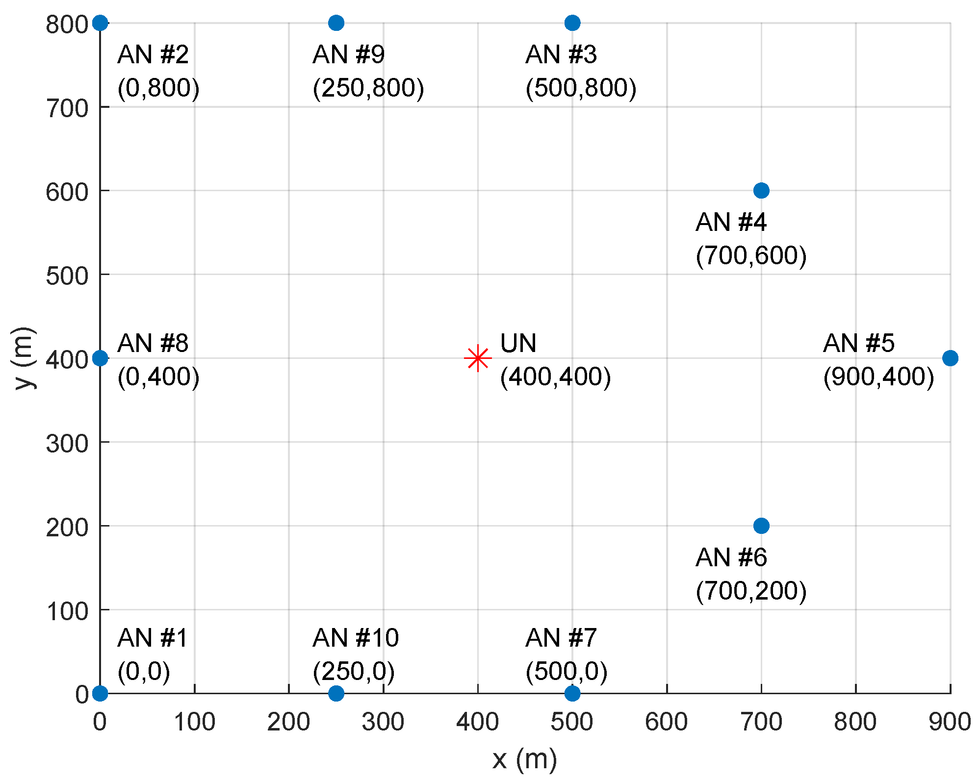
5. Numerical Results

Consider a large warehouse that uses automatic guided vehicles (AGVs) for cargoes. The AGVs are treated as independent UNs that will locate themselves. To avoid network overload and lower the energy consumption, the communication between UNs and ANs is one-way and sequential, so the one-way sequential TOAs are measurable. Therefore, simulation experiments shall be carried out in a scenario where $N=2$. Ten anchor nodes are deployed at ${\mathbf{s}}_1^o={[0,0]}^T$ m, ${\mathbf{s}}_2^o={[0,800]}^T$ m, ${\mathbf{s}}_3^o={[500,800]}^T$ m, ${\mathbf{s}}_4^o={[700,600]}^T$ m, ${\mathbf{s}}_5^o={[900,400]}^T$ m, ${\mathbf{s}}_6^o={[700,200]}^T$ m, ${\mathbf{s}}_7^o={[500,0]}^T$ m, ${\mathbf{s}}_8^o={[0,400]}^T$ m, ${\mathbf{s}}_9^o={[250,800]}^T$ m, and ${\mathbf{s}}_{10}^o={[250,0]}^T$ m. The true position of the user node is denoted as ${\mathbf{p}}^o={[400,400]}^T$ m. The geometric deployment is shown in Figure 4. The velocity of a UN is randomly generated within the range of 0 to 50 m/s, and the moving direction is random as well. ANs transmit signals sequentially with a fixed time interval of 5 ms; thus, $t_i=5(i-1)\times {10}^{-3}$ s. For each simulation test, the initial clock offset and clock drift of the UN are selected from uniform distributions. Specifically, the initial clock offset $\gamma$ follows a distribution of $\mathcal{U}(-{10}^{-5},{10}^{-5})$ s, while the clock drift $\iota$ follows a distribution of $\mathcal{U}(-20,20)$ parts per million (ppm). The known clock offsets ${\gamma }_i$, $i=1,2,\cdots ,M$ between ANs were also random in each test, obeying $\mathcal{U}(-{10}^{-5},{10}^{-5})$ s. The covariance matrices of the measurement noise and anchor position errors were set as ${\mathbf{Q}}_{\epsilon }={\sigma }^2{\mathbf{I}}_M$ and ${\mathbf{Q}}_s={\sigma }_s^2{\mathbf{I}}_{2M}$. Comparisons were conducted among the proposed CFPS (39), RIS (65), MLE implemented using GN iteration [9], and Guo’s CFJLAS [11]. Both the RIS and GN were initialized through the CFPS. The performance was evaluated using the RMSE and bias. Additionally, we utilized the CRLB as a benchmark for the performance evaluation. The ensemble runs for assessing the RMSE and bias was $T=1000$, unless specified otherwise. The RMSE and bias are defined as

$$\begin{array}{cc}\hfill RMSE\left(\mathbf{p}\right)& =\sqrt{\frac{1}{T}\sum _{t=1}^T{\parallel {\mathbf{p}}^{\left(t\right)}-{\mathbf{p}}^o\parallel }^2}\hfill \end{array}$$

(84)

$$\begin{array}{cc}\hfill RMSE\left(\mathbf{v}\right)& =\sqrt{\frac{1}{T}\sum _{t=1}^T{\parallel {\mathbf{v}}^{\left(t\right)}-{\mathbf{v}}^o\parallel }^2}\hfill \end{array}$$

(85)

$$\begin{array}{cc}\hfill bias\left(\mathbf{p}\right)& =\sqrt{\frac{1}{T}\sum _{t=1}^T\parallel {\mathbf{p}}^{\left(t\right)}-{\mathbf{p}}^o\parallel }\hfill \end{array}$$

(86)

$$\begin{array}{cc}\hfill bias\left(\mathbf{v}\right)& =\sqrt{\frac{1}{T}\sum _{t=1}^T\parallel {\mathbf{v}}^{\left(t\right)}-{\mathbf{v}}^o\parallel }\hfill \end{array}$$

(87)

where ${\mathbf{p}}^{\left(t\right)}$ and ${\mathbf{v}}^{\left(t\right)}$ are the estimation result at the t-th test. The maximum number of iterations for the RIS and GN is $K=100,000$, and the iteration residual threshold was set as $ϵ$ = 0.1.

We first evaluated the RMSE and bias performance under varying noise levels. The position error level of the ANs was fixed at ${\sigma }_s=0.5$ m. After testing the dumping factor $\kappa$ from 0 to 5, the results allowed us to determine the optimal selection. We chose $\kappa$ = 1 to yield the most favorable results, striking a balance between reducing divergence and maintaining convergence speed. The performance in terms of the RMSE and bias is illustrated in Figure 5, Figure 6, Figure 7 and Figure 8. The compared solutions can achieve CRLB accuracy when the noise is small, except the CFPS. It is reasonable that the CFPS ignores the inner connection between the redundant variables. The RIS can keep the CRLB’s level of accuracy when the noise reaches 30 dB, and slightly deviates from the CRLB if the noise increases further. The RMSE of the RIS is about 7 dB lower than that of CFJLAS when $10{log}_{10}\left({\sigma }^2\right)=35$ dB. The GN diverges from the CRLB when the noise level surpasses 25 dB, exhibiting a lower noise tolerance compared to the RIS. CFJLAS performs comparably to the RIS and GN when the noise is below 20 dB, but its RMSE deteriorates rapidly as the noise exceeds 20 dB. Regarding the bias, the RIS, GN, and CFJLAS behave at the same level if the noise is not significant. CFJLAS gradually deviates from the others, due to it applying the first-order Taylor expansion that drops the noise terms higher than the first order. The influence of dropping higher-order noise terms is reasonable and does not affect the performance since they are not significant if the noise is relatively small. However, when the noise is large where the higher-order noise terms cannot be neglected, the approximation error may dominate the performance, leading to rapid deterioration. The GN suffers from the divergence problem after 30 dB. The RIS is the best, and the bias of the RIS is better than that of its counterparts in large noise regions.

Next, we investigate the performance behavior as the position errors of the ANs change. The noise is fixed at 0 dB, and the variance of the AN position error varies from 10 to ${10}^5$ m². The RMSE and bias of each algorithm are illustrated in Figure 9, Figure 10, Figure 11 and Figure 12. When the error level is below ${10}^{3.5}$, the RMSE of the RIS, GN, and CFJLAS achieve the CRLB. However, if ${\sigma }_s^2>{10}^{3.5}$ m², the RMSE of the GN diverges from the CRLB, and CFJLAS begins to deviate from the CRLB. The RIS maintains a performance close to the CRLB, demonstrating that it is better than the GN and CFJLAS. The bias behaves similar to the RMSE. The biases of the RIS, GN, and CFJLAS are comparable under the small-error condition, but the RIS shows its superiority if the error is significant.

The simulations validated that the RIS is robust to measurement noise and position errors of ANs compared to the methods. We then investigated the performance of the RIS through convergence, comparing it to the GN, the other iterative solution. Convergence is obtained if the residual between adjacent iterations reaches the threshold $\parallel {\widehat{\mathit{\mu }}}^{(k+1)}(1:2N)-{\widehat{\mathit{\mu }}}^{\left(k\right)}(1:2N)\parallel <ϵ$. ${\wp }_{ϵ}$ is the probability of attaining the threshold. The maximum number of iterations was set to 100,000, and the threshold $ϵ$ was set to 0.01. In each trial, the initial estimate ${\mathit{\mu }}^{\left(0\right)}$ was randomly generated as ${\mathit{\mu }}^{\left(0\right)}={\mathit{\mu }}^o+e\Delta \mathcal{x}$, where e represents the error coefficient. $\Delta \mathcal{x}$ is a $2N+2$-dimensional random vector, where the 1 to N, $N+1$ to $2N$, $2N+1$-th, and $2N+2$-th elements are uniformly distributed within the range $(-0.5,0.5)$ m, $(-0.05,0.05)$ m/s, $(-5,5)$ ns, and $(-0.05,0.05)$ ppm. e was fixed at 100. The error ${\sigma }_s$ was set as 0.5 m. Figure 13 reveals the convergence probability as the noise level increases. When the noise is relatively low, such as below 35 dB, both the RIS and GN converge to the threshold $ϵ$ with probability 1. However, as the noise increases, the RIS still maintains a significantly high convergence probability that is over 80%. Compared to the GN’s results, the RIS’s results highlight the superior robustness of the RIS and explain the reason why the RMSEs in Figure 5 and Figure 9 of the RIS are the best.

The RIS was also found to be resilient to an initial guess. The next simulation fixed the noise and AN position error levels at 10 dB and 0.25 m² and examined the influence of the initialization error by varying e from 10 m to ${10}^4$ m. The other parameters remained the same as in the previous settings. The convergence probability is shown in Figure 14. Figure 14 indicates that the RIS exhibits a higher convergence probability, even when the initial point is distant from the true value. For instance, when e equals ${10}^{3.5}$ m, the RIS method still achieves a convergence probability of 1, whereas the GN method fails to do so. This simulation experiment validates that the RIS is robust to an initial guess. Therefore, although the CFPS cannot provide an accurate solution to start the RIS, it can converge to the optimal and perform better than the GN.

We also evaluated the performance as the number of ANs varies. The AN positions were selected from

Table 3. Positions of ANs.

Anchor	Position	Anchor	Position
AN #1	${[0,0]}^T$m	AN #8	${[0,400]}^T$m
AN #2	${[0,800]}^T$m	AN #9	${[250,800]}^T$m
AN #3	${[500,800]}^T$m	AN #10	${[250,0]}^T$m
AN #4	${[700,600]}^T$m	AN #11	${[0,600]}^T$m
AN #5	${[900,400]}^T$m	AN #12	${[0,200]}^T$m
AN #6	${[700,200]}^T$m	AN #13	${[400,800]}^T$m
AN #7	${[500,0]}^T$m	AN #14	${[600,450]}^T$m

, with the first M ANs used for testing. The noise power and position error of ANs are set to ${\sigma }^2=0.1$ m² and ${\sigma }_s^2=1$ m², respectively. Notably, the number of unknowns in the first stage is $2N+4$, and the number of equations is $M-1$. Therefore, the minimum number of ANs must satisfy $M-1\ge 2N+4$. For the simulation scenario with $N=2$, we start with $M=9$ ANs. Figure 15, Figure 16, Figure 17 and Figure 18 show the RMSE and bias performances of all compared solutions, which improve as the number of ANs increases. The accuracy of theh CFPS declines significantly when M is less than 10, yet it still provides a satisfactory initial guess, ensuring that the RIS converges to an optimum. Processing times are depicted in Figure 19, confirming the analytical results in Section 4.3. The computational complexity rises with an increasing number of ANs. It is important to note that the processing times for the RIS and GN are similar in Figure 19, differing from those in

Table 4. Processing times of compared solutions.

Method	RIS	GN	CFPS	CFJLAS
Times (s)	60.2648	26.6622	1.8245	2.7523
Rel. Times	21.89	9.69	0.66	1

of Section 5. This is because both the RIS and GN converge after a similar number of iterations due to the relatively low noise power and position error.

The computational times of generating the results in Figure 5, Figure 6, Figure 7 and Figure 8 were recorded by Matlab 2022 on a typical personal computer with an AMD 5800H CPU @3.2 GHz, with 16 G of RAM and an AMD Radeon Vega8 GPU. The processing times and relative processing times are depicted in Table 4. Although the RIS is more robust than the GN in measurement noise, AN position error, and initial guess, the processing times of the RIS and GN are comparable. The RIS requires $226\%$ more time than the GN, but the computational load is on the same order of magnitude. Again, we confirm the superior performance of the RIS, particularly under large-noise/error conditions or poor initialization, but the complexity is manageable.

6. Conclusions

This study investigated the JLAS problem for mobile UNs using sequential one-way TOA measurements. We formulate the JLAS as a CWLS optimization problem, addressing it by projecting the equation into the nullspace of the redundant variables introduced during pseudo-linearization, resulting in a coarse solution. A refinement step follows to enhance accuracy, and this solution is termed CFPS. As CFPS is suboptimal, we propose an RIS from the perspective of FG. Through introducing a damping factor into the iteration, the robustness to measurement noise, position errors of the ANs, and initial guess are significantly enhanced. Theoretical analysis proves that the proposed RIS can attain the CRLB when the noise and errors are mild. Simulations validated the analytical results and demonstrated the superiority of the RIS in terms of the RMSE, bias, and convergence probability. The RIS can maintain CRLB-level RMSEs even when the noise or error is relatively large and exhibits a lower bias than current solutions. It also has a higher probability of convergence than the GN, making it less sensitive to initial guesses. Despite the RIS’s better performance compared to existing solutions, its computational complexity does not increase significantly, remaining on the same magnitude as the GN and CFJLAS. This work assumed that ANs are static and that the clock offset of each AN is perfectly known. Future research interests may include JLAS using moving ANs, anchor node placement optimization, and mitigating unknown AN clock offsets. Another challenge is high AN position uncertainty or high measurement noise, which can occur in practical applications. While the proposed RIS significantly improves robustness to AN position uncertainty and measurement noise, further study is needed in this area.

References

1. Gonçalves Ferreira, A.F.G.; Fernandes, D.M.A.; Catarino, A.P.; Monteiro, J.L. Localization and Positioning Systems for Emergency Responders: A Survey. IEEE Commun. Surv. Tut. 2017, 19, 2836–2870. [Google Scholar] [CrossRef]
2. Farahsari, P.S.; Farahzadi, A.; Rezazadeh, J.; Bagheri, A. A Survey on Indoor Positioning Systems for IoT-Based Applications. IEEE Internet Things J. 2022, 9, 7680–7699. [Google Scholar] [CrossRef]
3. Yang, H.; Zhong, W.D.; Chen, C.; Alphones, A. Integration of Visible Light Communication and Positioning within 5G Networks for Internet of Things. IEEE Netw. 2020, 34, 134–140. [Google Scholar] [CrossRef]
4. Wen, F.X.; Wymeersch, H.; Peng, B.L.; Tay, W.P.; So, H.C.; Yang, D.G. A survey on 5G massive MIMO localization. Digit. Signal Process. 2019, 94, 21–28. [Google Scholar] [CrossRef]
5. Saeed, N.; Alouini, M.S.; Al-Naffouri, T.Y. 3D Localization for Internet of Underground Things in Oil and Gas Reservoirs. IEEE Access 2019, 7, 121769–121780. [Google Scholar] [CrossRef]
6. Tabella, G.; Ciuonzo, D.; Paltrinieri, N.; Rossi, P.S. Bayesian Fault Detection and Localization Through Wireless Sensor Networks in Industrial Plants. IEEE Internet Things J. 2024, 11, 13231–13246. [Google Scholar] [CrossRef]
7. Shi, Q.; Cui, X.; Zhao, S.; Lu, M. Sequential TOA-Based Moving Target Localization in Multi-Agent Networks. IEEE Commun. Lett. 2020, 24, 1719–1723. [Google Scholar] [CrossRef]
8. Zhao, S.; Zhang, X.P.; Cui, X.; Lu, M. Optimal Localization with Sequential Pseudorange Measurements for Moving Users in a Time-Division Broadcast Positioning System. IEEE Internet Things J. 2021, 8, 8883–8896. [Google Scholar] [CrossRef]
9. Zhao, S.; Zhang, X.P.; Cui, X.; Lu, M. Optimal Two-Way TOA Localization and Synchronization for Moving User Devices with Clock Drift. IEEE Trans. Veh. Technol. 2021, 70, 7778–7789. [Google Scholar] [CrossRef]
10. Zhao, S.; Guo, N.; Zhang, X.P.; Cui, X.; Lu, M. Closed-Form Two-Way TOA Localization and Synchronization for User Devices with Motion and Clock Drift. IEEE Signal Process. Lett. 2022, 29, 100–104. [Google Scholar] [CrossRef]
11. Guo, N.; Zhao, S.; Zhang, X.P.; Yao, Z.; Cui, X.; Lu, M. New Closed-Form Joint Localization and Synchronization Using Sequential One-Way TOAs. IEEE Trans. Signal Process. 2022, 70, 2078–2092. [Google Scholar] [CrossRef]
12. Rui, L.; Ho, K.C. Algebraic Solution for Joint Localization and Synchronization of Multiple Sensor Nodes in the Presence of Beacon Uncertainties. IEEE Trans. Wirel. Commun. 2014, 13, 5196–5210. [Google Scholar] [CrossRef]
13. Goodarzi, M.; Sark, V.; Maletic, N.; Terán, J.G.; Caire, G.; Grass, E. DNN-Assisted Particle-Based Bayesian Joint Synchronization and Localization. IEEE Trans. Commun. 2022, 70, 4837–4851. [Google Scholar] [CrossRef]
14. Ge, T.; Tharmarasa, R.; Lebel, B.; Florea, M.; Kirubarajan, T.T. A Multidimensional TDOA Association Algorithm for Joint Multitarget Localization and Multisensor Synchronization. IEEE Trans. Aerosp. Electron. Syst. 2020, 56, 2083–2100. [Google Scholar] [CrossRef]
15. Kazemi, S.A.R.; Amiri, R.; Behnia, F. Efficient Joint Localization and Synchronization in Distributed MIMO Radars. IEEE Signal Process. Lett. 2020, 27, 1200–1204. [Google Scholar] [CrossRef]
16. Shams, R.; Otero, P.; Aamir, M.; Hanif, F. E2JSL: Energy Efficient Joint Time Synchronization and Localization Algorithm Using Ray Tracing Model. Sensors 2020, 20, 7222. [Google Scholar] [CrossRef] [PubMed]
17. Myung, H.G.; Lim, J.; Goodman, D.J. Single carrier FDMA for uplink wireless transmission. IEEE Veh. Technol. Mag. 2006, 1, 30–38. [Google Scholar] [CrossRef]
18. Picois, A.V.; Samama, N. Near-far interference mitigation for pseudolites using double transmission. IEEE Trans. Aerosp. Electron. Syst. 2014, 50, 2929–2941. [Google Scholar] [CrossRef]
19. Shi, Q.; Cui, X.; Zhao, S.; Xu, S.; Lu, M. BLAS: Broadcast Relative Localization and Clock Synchronization for Dynamic Dense Multiagent Systems. IEEE Trans. Aerosp. Electron. Syst. 2020, 56, 3822–3839. [Google Scholar] [CrossRef]
20. Dwivedi, S.; Zachariah, D.; De Angelis, A.; Handel, P. Cooperative Decentralized Localization Using Scheduled Wireless Transmissions. IEEE Commun. Lett. 2013, 17, 1240–1243. [Google Scholar] [CrossRef]
21. Hamer, M.; D’Andrea, R. Self-Calibrating Ultra-Wideband Network Supporting Multi-Robot Localization. IEEE Access 2018, 6, 22292–22304. [Google Scholar] [CrossRef]
22. Zachariah, D.; De Angelis, A.; Dwivedi, S.; Händel, P. Self-Localization of Asynchronous Wireless Nodes with Parameter Uncertainties. IEEE Signal Process. Lett. 2013, 20, 551–554. [Google Scholar] [CrossRef]
23. Carroll, P.; Mahmood, K.; Zhou, S.; Zhou, H.; Xu, X.; Cui, J.H. On-Demand Asynchronous Localization for Underwater Sensor Networks. IEEE Trans. Signal Process. 2014, 62, 3337–3348. [Google Scholar] [CrossRef]
24. Yan, J.; Zhang, X.; Luo, X.; Wang, Y.; Chen, C.; Guan, X. Asynchronous Localization with Mobility Prediction for Underwater Acoustic Sensor Networks. IEEE Trans. Veh. Technol. 2018, 67, 2543–2556. [Google Scholar] [CrossRef]
25. Sun, M.; Yang, L. On the joint time synchronization and source localization using TOA measurements. Int. J. Distrib. Sens. Netw. 2013, 9, 794805. [Google Scholar] [CrossRef]
26. Zhao, S.; Zhang, X.P.; Cui, X.; Lu, M. Semidefinite Programming Two-Way TOA Localization for User Devices with Motion and Clock Drift. IEEE Signal Process. Lett. 2021, 28, 578–582. [Google Scholar] [CrossRef]
27. Yu, Q.; Wang, Y.; Shen, Y. Joint Localization and Synchronization for Moving Agents Using One-Way TOAs in Asynchronous Networks. IEEE Internet Things J. 2023, 10, 11844–11857. [Google Scholar] [CrossRef]
28. Sun, Y.; Ho, K.C.; Wan, Q. Solution and Analysis of TDOA Localization of a Near or Distant Source in Closed-Form. IEEE Trans. Signal Process. 2019, 67, 320–335. [Google Scholar] [CrossRef]
29. Jia, T.Y.; Liu, H.W.; Ho, K.C.; Wang, H.Y. Mitigating Sensor Motion Effect for AOA and AOA-TOA Localizations in Underwater Environments. IEEE Trans. Wirel. Commun. 2023, 22, 6124–6139. [Google Scholar] [CrossRef]
30. Zou, Y.; Fan, J.; Wu, L.; Liu, H. Fixed Point Iteration Based Algorithm for Asynchronous TOA-Based Source Localization. Sensors 2022, 22, 6871. [Google Scholar] [CrossRef]
31. Yu, Z.; Li, J.; Guo, Q.; Sun, T. Message Passing Based Robust Target Localization in Distributed MIMO Radars in the Presence of Outliers. IEEE Signal Process. Lett. 2020, 27, 2168–2172. [Google Scholar] [CrossRef]
32. Yu, Z.; Li, J.; Guo, Q.; Ding, J. Efficient Direct Target Localization for Distributed MIMO Radar with Expectation Propagation and Belief Propagation. IEEE Trans. Signal Process. 2021, 69, 4055–4068. [Google Scholar] [CrossRef]
33. Yu, Z.; Li, J.; Guo, Q. Message Passing Based Target Localization Under Range Deception Jamming in Distributed MIMO Radar. IEEE Signal Process. Lett. 2021, 28, 1858–1862. [Google Scholar] [CrossRef]
34. Sun, Y.; Ho, K.C.; Yang, Y.; Zhang, L.; Chen, L. Robust Iterative Solution for Linear Array-Based 3-D Localization by Message Passing. In Proceedings of the ICASSP 2023—2023 IEEE International Conference on Acoustics, Speech and Signal Processing (ICASSP), Rhodes Island, Greece, 4–10 June 2023; pp. 1–5. [Google Scholar]
35. Zhang, Z.; Shi, Z.; Gu, Y.; Greco, M.S.; Gini, F. Ziv-Zakai Bound for Compressive Time Delay Estimation From Zero-Mean Gaussian Signal. IEEE Signal Process. Lett. 2023, 30, 1112–1116. [Google Scholar] [CrossRef]
36. Zhang, Z.; Shi, Z.; Zhou, C.; Yan, C.; Gu, Y. Ziv-Zakai Bound for Compressive Time Delay Estimation. IEEE Trans. Signal Process. 2022, 70, 4006–4019. [Google Scholar] [CrossRef]
37. Zhang, Z.; Shi, Z.; Shao, C.; Chen, J.; Greco, M.S.; Gini, F. Ziv-Zakai Bound for 2D-DOAs Estimation. IEEE Trans. Signal Process. 2024, 72, 2483–2497. [Google Scholar] [CrossRef]
38. Kay, S.M. Fundamentals of Statistical Signal Processing: Estimation Theory; Prentice-Hall: Englewood Cliffs, NJ, USA, 1993. [Google Scholar]
39. Bernstein, D.S. Matrix mathematics: Theory, Facts, and Formulas with Application to Linear Systems Theory; Princeton University Press: Princeton, NJ, USA, 2005. [Google Scholar]
40. Wu, L.; Sahu, N.; Xu, S.; Babu, P.; Ciuonzo, D. Optimization Based Sensor Placement for Multi-Target Localization with Coupling Sensor Clusters. IEEE Trans. Signal Inf. Process. Netw. 2023, 9, 596–611. [Google Scholar] [CrossRef]
Figure 1. Localization scenario of JLAS system using the TD broadcasting scheme.
Applsci 14 06069 g001
Figure 2. Factor graph of sequential TOA JLAS.
Applsci 14 06069 g002
Figure 3. Example of divergence behavior: position error of each iteration.
Applsci 14 06069 g003
Figure 4. ANs and UN in the simulation scene.
Applsci 14 06069 g004
Figure 5. The RMSE of the UN location estimation as the noise power increases.
Applsci 14 06069 g005
Figure 6. The bias of the UN location estimation as the noise power increases.
Applsci 14 06069 g006
Figure 7. The RMSE of the UN velocity estimation as the noise power increases.
Applsci 14 06069 g007
Figure 8. The bias of the UN velocity estimation as the noise power increases.
Applsci 14 06069 g008
Figure 9. The RMSE of the UN location estimation as the position error of the AN increases.
Applsci 14 06069 g009
Figure 10. The bias of the UN location estimation as the position error of the AN increases.
Applsci 14 06069 g010
Figure 11. The RMSE of the UN velocity estimation as the position error of the AN increases.
Applsci 14 06069 g011
Figure 12. The bias of the UN velocity estimation as the position error of the AN increases.
Applsci 14 06069 g012
Figure 13. Convergence probability as the noise power increases.
Applsci 14 06069 g013
Figure 14. Influence of initialization error on convergence.
Applsci 14 06069 g014
Figure 15. RMSE of the UN location estimation as the number of ANs increases.
Applsci 14 06069 g015
Figure 16. Bias of the UN location estimation as the number of ANs increases.
Applsci 14 06069 g016
Figure 17. RMSE of the UN velocity estimation as the number of ANs increases.
Applsci 14 06069 g017
Figure 18. Bias of the UN velocity estimation as the number of ANs increases.
Applsci 14 06069 g018
Figure 19. Processing times as the number of ANs increases.
Applsci 14 06069 g019