Non-Invasive Continuous Blood Pressure Estimation from Single-Channel PPG Based on a Temporal Convolutional Network Integrated with an Attention Mechanism

Abstract

Traditional cuff-based blood pressure measurement methods suffer from issues such as intermittency and applicability, while cuff-less continuous blood pressure estimation techniques are increasingly gaining attention due to their non-invasive and continuous monitoring advantages. In this paper, aiming at the challenges faced by existing cuff-less continuous blood pressure estimation models in terms of accuracy, data requirements, and generalization ability, a series of innovative approaches are proposed. Deep learning techniques are introduced to design an end-to-end blood pressure estimation model with high accuracy, ease of training, and strong generalization ability. To address the insufficient accuracy of traditional neural networks in cuff-less continuous blood pressure estimation, we propose an end-to-end, beat-to-beat blood pressure estimation model that combines the temporal convolutional network (TCN) and convolutional block attention module (CBAM). By enhancing the model’s ability to process time series data and focus on key features of photoplethysmography (PPG), the blood pressure estimation accuracy during the resting state is significantly improved. The absolute mean error and standard deviation of systolic blood pressure (SBP) estimation using the algorithm in this chapter on the University of California, Irvine (UCI) physiological signal dataset are 5.3482 mmHg and 8.3410 mmHg, respectively, which are superior to other deep learning models based on convolutional neural network and recurrent neural network architectures.

1. Introduction

Blood pressure stands as a crucial indicator for assessing the health status of the cardiovascular system, with its fluctuations reflecting changes in bodily functions and the progression of various ailments. As per a World Health Organization report, as of 2021, a staggering 1.28 billion adults globally were afflicted with hypertension. However, alarmingly, less than half of these adult hypertensive patients had received a diagnosis and treatment. Consequently, hypertension claims the lives of over 10 million people worldwide annually [1]. Hence, precise blood pressure monitoring holds immense significance in preventing cardiovascular diseases and elevating human health standards.

Currently, traditional blood pressure measurement methods primarily include cuff-based blood pressure measurement and continuous blood pressure monitoring. However, cuff-based measurements can be significantly affected by factors such as cuff size, measurement environment, and operator skill, potentially leading to considerable errors [2]. Additionally, this method only provides a snapshot of blood pressure at a specific moment, making it impossible to continuously track blood pressure changes. In contrast, continuous blood pressure monitoring offers a more precise assessment of a patient’s blood pressure status, including fluctuations during exercise and changes in blood pressure during the night. This approach aids doctors in accurately diagnosing patients’ conditions and devising more tailored treatment plans. It allows for the timely detection of blood pressure variations and enables the adoption of necessary measures to control the progression of hypertension and other cardiovascular diseases. This holds immense significance in preventing cardiovascular and cerebrovascular events and reducing disease risks. Nevertheless, existing continuous blood pressure monitoring methods often require invasive devices like intravascular catheters, which are not only cumbersome to operate but also prone to infections and other complications [3]. Given the limitations and shortcomings of these traditional blood pressure measurement techniques in practical applications, there is an urgent need for a non-invasive, continuous, and accurate blood pressure measurement method.

In recent years, advancements in sensing technology, computer science, and artificial intelligence have spurred increasing numbers of researchers to explore continuous blood pressure estimation methods utilising biosignals such as PPG and electrocardiogram (ECG). When juxtaposed with conventional blood pressure measurement techniques, these novel approaches exhibit various advantages, including real-time continuous monitoring, non-invasiveness, and user-friendliness [4]. Numerous notable achievements have been attained in studies focused on estimation methodologies that integrate PPG and ECG data, showcasing impressive accuracy in blood pressure estimations. Nonetheless, there are certain drawbacks associated with ECG signal measurement. Specifically, it necessitates the prolonged attachment of patch electrodes to the skin, which can hinder skin ventilation and induce discomfort for the user [5]. Furthermore, blood pressure estimation techniques relying on multiple physiological signals, including ECG and PPG, encounter challenges related to data synchronisation, information fusion, elevated development costs, complex implementation, and limited noise resistance [6]. In contrast, methodologies solely reliant on a single PPG signal offer a streamlined approach, eliminating the complexities and inconveniences associated with multiple sensors. This approach simplifies the data collection and processing workflow. Additionally, as the PPG signal is typically captured from the fingertip, it provides a more stable measurement point compared to multi-channel PPG signal acquisition, making it particularly suitable for extended blood pressure monitoring sessions.

To better grasp the long-term correlation between PPG signals and blood pressure values, and to enhance the precision and robustness of continuous blood pressure estimation on large-scale public datasets, this paper introduces a method that integrates a CBAM into a TCN for continuous blood pressure estimation. Our approach employs one-dimensional convolutional modules alongside the CBAM for comprehensive signal feature extraction and fusion. Additionally, we use dilated and causal convolutions to decipher the temporal dependencies between blood pressure and PPG waveforms. Experimental results on public datasets indicate that our method notably improves blood pressure estimation accuracy when compared to traditional machine learning models and deep learning models rooted in the CNN-RNN framework. Moreover, it excels at capturing abrupt changes in blood pressure. The primary contributions of this study are outlined below:

(1)

This paper introduces dilated convolution and causal convolution from TCN to effectively learn the temporal dependencies between blood pressure and PPG waveforms.

(2)

Integration of CBAM module: To further enhance the performance of feature extraction, this method incorporates the CBAM module into the one-dimensional convolutional module.

(3)

Experimental validation on large-scale public datasets: This study employs large-scale public datasets for experimental evaluation, aiming to ensure the robustness of continuous blood pressure estimation across diverse samples and scenarios.

2. Related Works

For the non-invasive continuous blood pressure estimation task using single-channel PPG, existing methodologies can be broadly categorised into traditional machine learning and deep learning approaches. Traditional machine learning techniques often entail manual feature extraction from raw PPG data, followed by the development of a regression model based on conventional machine learning algorithms to estimate systolic and diastolic blood pressure in individuals. For instance, Teng Xiaofei et al. [7] selected specific features from the PPG signal, such as the half-width and two-thirds width of the pulse amplitude, systolic ascending time, and diastolic time, to establish a linear regression model for estimating systolic and diastolic blood pressure. Their method demonstrated impressive accuracy on a dataset comprising 15 young and healthy subjects. In another study, Yuriy Kurylyak et al. [8] extracted 21 parameters from over 15,000 heartbeat training samples in the Multiparameter Intelligent Monitoring in Intensive Care (MIMIC) database. These parameters served as input features for an Artificial Neural Network (ANN) aimed at estimating blood pressure from PPG signals. This approach proved to be more precise than the linear regression method. Liu et al. [9] extracted 14 features from the second derivative of PPG (SDPPG) and combined them with the 21 features used by Kurylyak et al. They employed a support vector machine as a BP estimator to improve the prediction of systolic and diastolic blood pressure. Compared to the 21 features and ANN applied by Kurylyak et al., this approach enhanced the accuracy of BP estimation by 40%. The primary challenge faced by methods that use manual features and classic machine learning for blood pressure estimation lies in the requirement for high-quality PPG signals to accurately locate PPG waveform feature points. However, PPG signals collected by wearable devices often contain significant noise and motion artefacts, making it difficult to accurately identify critical feature points such as peaks, valleys, dicrotic notches, and inflection points. Consequently, a series of features derived from the positions of these feature points also suffer from considerable errors. Additionally, the design and selection of manual features require professional knowledge and experience and often involve multiple trials to determine the optimal feature set, posing certain limitations in practical applications.

With the steady enhancement of computing power, researchers have shifted their focus towards automatic feature extraction methods for PPG signals utilising deep learning techniques [10]. In contrast to traditional machine learning models, deep learning models excel at learning features directly from raw data, eliminating the need for manual feature extraction and harnessing the latent information embedded within the raw signals. The most prevalent models can be broadly categorised into convolutional neural networks (CNNs), recurrent neural networks (RNNs), and hybrids of CNN and RNN. Baek et al. [11] introduced a method that leverages both the time and frequency domains of PPG signals as inputs, employing a CNN framework to forecast BP without requiring explicit feature extraction. When tested on a dataset comprising 26 volunteers, the approach yielded a total mean absolute error (MAE) of 5.28 mmHg and 4.92 mmHg for estimated systolic and diastolic blood pressure, respectively. Peng Su and team [12] reformulated BP estimation as a sequence prediction challenge, utilising a deep recurrent neural network to model the temporal dependencies inherent in BP dynamics. Their experiments, conducted on a dataset of 84 healthy subjects, revealed that their model surpassed the accuracy of conventional BP prediction models. While these studies demonstrated impressive performance on smaller datasets, findings from similar investigations on larger public datasets differed. Slapnicar et al. [13] employed both convolutional and recurrent neural networks to process the time and frequency domain information of PPG signals, amalgamating the extracted features to estimate systolic and diastolic blood pressure. Their tests on a dataset of 510 subjects from the MIMIC III database resulted in mean absolute errors of 9.43 mmHg and 6.88 mmHg for systolic and diastolic blood pressure estimations, respectively. However, these estimations fell short of the precision standards set by the Advancement of Medical Instrumentation (AAMI) and British Hypertension (BHI). In another study, Fabian Schrumpf et al. [14] extracted PPG and ambulatory blood pressure signal records from 4000 patients in the MIMIC-III database. They evaluated the performance of four deep learning models—AlexNet, ResNet, Slapnicar’s proposed model, and BiLSTM—in continuous blood pressure estimation tasks. Notably, AlexNet and ResNet are based on the CNN architecture, BiLSTM leverages the RNN architecture, and Slapnicar’s model integrates both CNN and RNN elements. Their findings indicated that none of these models met the blood pressure measurement accuracy requirements outlined by the Association for the AAMI [15] or the British Hypertension Society (BHS) [16]. Consequently, these models are not yet ready for clinical use, unlike traditional cuff-based blood pressure monitoring devices.

3. Materials

3.1. Dataset Introduction

The data used in this study are sourced from the “Cuff-Less Blood Pressure Estimation Data Set” in the UCI database [17]. This dataset is a subset of the Multiparameter Intelligent Monitoring in Intensive Care (MIMIC) II online waveform database, containing 12,000 clinical vital sign records of intensive care unit (ICU) patients screened by KaChuee et al. [17] from MIMIC-II. The patients came from different geographical areas and demographic backgrounds to ensure the diversity and generality of the data. Each record in this dataset consists of PPG, ECG, and arterial blood pressure (ABP) signals recorded by a multiparameter monitor in the ICU, with a sampling rate of 125 Hz and sampling durations ranging from 8 s to 10 min. KaChuee et al. performed simple cleaning on the original signals using methods such as moving average filtering and removing abnormal segments, eliminating some records with poor signal quality. The dataset is stored in Matlab’s v7.3 mat file format.

3.2. Baseline Drift Elimination

In the UCI dataset, Kachuee et al. [17] performed moving average filtering on the raw PPG signals and eliminated segments with severe discontinuities or large periodic differences. However, they did not address the common issue of baseline wander present in the raw signals. Baseline wander is caused by various factors such as respiration, changes in body position, and temperature variations. It leads to an overall upward or downward trend in the PPG signal, resulting in scale transformations that make it difficult to compare and match different PPG signal cycles. Additionally, baseline wander introduces extra noise and interference, reducing the signal-to-noise ratio of the PPG signal and increasing the error and uncertainty of blood pressure estimation models. Therefore, it is necessary to perform baseline wander correction on the PPG signal to eliminate its impact on model predictions and improve the accuracy and stability of the model. In this study, the variational mode decomposition (VMD) [18] algorithm is employed to remove baseline wander from the raw signals. VMD is a signal decomposition method based on the idea of representing a signal as a series of locally frequency-modulated components, with each component corresponding to a mode. Each mode function has a specific centre frequency and bandwidth, allowing it to capture different frequency components in the signal. By summing these mode functions, the original signal can be reconstructed. The low-frequency intrinsic mode functions (IMFs) obtained through the VMD decomposition of the signal typically contain information about baseline wander. By selecting the low-frequency IMFs and subtracting them from the original signal, baseline wander can be removed. The process of using the VMD algorithm to remove baseline drift is as follows:

Define the original signal as x(t), where t represents time. This step involves an iterative optimization process that calculates IMFs and residual terms by minimizing a set of constrained optimization problems. The optimization problem of the VMD algorithm can be expressed as:

$${min\sum _{\mathrm{i}}{\left|{\mathrm{A}}_{\mathrm{n}\mathrm{i}}\otimes {\mathrm{u}}_{\mathrm{n}}-\mathrm{x}\left(\mathrm{t}\right)\right|}^2+\lambda \sum _{\mathrm{i}}\int {\left|\partial {\mathrm{t}\mathrm{u}}_{\mathrm{p}}\left(\mathrm{t}\right)\right|}^2\mathrm{d}\mathrm{t}}^2$$

(1)

where Aₙᵢ is the envelope function of each IMF, uₙ is the phase function of each IMF, and λ is the regularization parameter. The first term represents the signal reconstruction error, while the second term is the regularization term used to constrain the smoothness of the IMFs. Through an iterative optimization process, a set of IMFs and a residual term are obtained. The IMFs have different frequencies and bandwidths, where the low-frequency IMF captures the slow-changing component of baseline wander, while the high-frequency IMF captures faster changes. Here, we choose the low-frequency IMF as an approximation of baseline wander and subtract it from the original signal. The resulting signal after removing baseline wander is shown in Figure 1. It can be seen that there is an obvious baseline wander in the original PPG signal, and the overall signal offset is very similar to the trend of the low-frequency IMF obtained using VMD decomposition. After decomposing the original signal using the VMD algorithm, removing the low-frequency components, and reconstructing it, the periodicity of the new signal becomes more pronounced.

3.3. Signal Segmentation

To ensure dataset balance, it is necessary to guarantee that the recording durations for each subject used in the study are roughly equivalent. Therefore, all records with durations shorter than 8 min were excluded. Subsequently, we segmented the PPG and ABP recordings into several signal segments using a 10-second window. Blood pressure systolic and diastolic pressures represent the maximum and minimum pressures exerted on the blood vessel walls during heart contraction and relaxation, respectively. The representativeness of these two indicators makes them crucial parameters for assessing an individual’s cardiovascular health and developing treatment plans. We processed each ABP signal frame using a peak and valley detection algorithm to extract SBP and diastolic blood pressure (DBP). SBP is defined as the amplitude of the main peak in a complete ABP signal cycle, while DBP is the amplitude of the trough adjacent to and preceding the main peak. To avoid interference from extremely high or low blood pressure in extracting general relationships from PPG-BP, we excluded records where systolic or diastolic blood pressure fell outside the normal range. After screening, we retained record segments with SBP values between 80 mmHg and 180 mmHg and DBP values between 60 mmHg and 130 mmHg. Following these processing steps, we obtained a total of 270,488 sample data points. Each data point contains an 8-second PPG signal and the corresponding SBP and DBP values. The distribution of SBP and DBP in the dataset is shown in Figure 2.

4. Methods

This study proposes a model based on a temporal convolutional network with a channel attention module (TCN-CBAM) for processing time series data. The goal of this model is to improve the modelling capabilities of long-term dependencies and channel correlations in PPG and blood pressure data, thereby enhancing the model’s expressive power and estimation performance.

As shown in Figure 3, the backbone of the model adopts a stacked structure of TCN residual blocks. Each residual block consists of multiple one-dimensional dilated causal convolutional layers designed to capture dependencies at different scales in time series data. The dilation rates of these convolutional layers gradually increase to capture longer-range dependencies. Meanwhile, batch normalization and exponential linear unit (ELU) activation functions are applied after each convolutional layer for normalization and nonlinear transformation. The spatial attention module weights each position of the time series data through a one-dimensional convolutional layer and a Sigmoid activation function. This allows the model to learn the importance weights of each position, capturing temporal correlations in the time series data. The final layer of the TCN-CBAM model is a fully connected layer that maps the output of the hidden layer to a two-dimensional vector containing SBP and DBP, yielding the final prediction results. By combining TCN and CBAM, our proposed model can effectively model long-term dependencies in time series data and apply weighting in both the channel and spatial dimensions, enhancing the model’s expressive power and prediction performance. This model has broad applications in time series data processing and analysis tasks.

4.1. Dilated Causal Convolution

The PPG signal, continuously collected over time, is a physiological indicator that reflects the filling and emptying processes of blood vessels. This process is intricately linked to heartbeats and fluctuations in blood pressure. Both PPG and ambulatory blood pressure signals possess periodic, autocorrelated, nonlinear, and non-stationary traits [19]. Consequently, cuff-less continuous blood pressure estimation solely based on PPG signals qualifies as a time series analysis. In previous investigations, RNNs and their variations, including long short-term memory (LSTM) and gate recurrent unit (GRU), have proven effective in capturing the temporal dependencies inherent in PPG signals, surpassing the accuracy achieved by conventional machine learning techniques and CNNs in blood pressure estimation. Nevertheless, conventional RNNs encounter challenges such as gradient vanishing or exploding when dealing with extended sequence data. Additionally, their serial computation nature hinders efficiency, restricting their applicability to extensive datasets. The emergence of TCNs [20] adeptly addresses the limitations of traditional RNNs in handling long sequences. By leveraging the architecture of convolutional neural networks, TCNs offer enhanced performance and broader applicability in sequence modelling endeavours.

Dilated causal convolution [21] stands as a pivotal component for harnessing the strengths of TCN. In the context of time series data, causal convolution signifies that the convolution kernel solely observes data preceding the present time step, preventing access to current or subsequent data. This precautionary measure ensures that the model refrains from utilizing future information when anticipating the present time step. Conversely, dilated convolution broadens [22] the receptive field of the kernel by introducing gaps in sampling, termed dilation factors, thereby facilitating the capture of more extended temporal dependencies. Dilated causal convolution [23] seamlessly integrates the attributes of both causal and dilated convolutions, effectively grasping long-term dependencies within time series data. Typically, the architecture of a dilated causal convolution block takes the following form.

A dilated causal convolution block showed in Figure 4 is a module composed of multiple dilated causal convolution layers, commonly used in the construction of network structures such as TCN. Each dilated causal convolution layer possesses distinct dilation factors but shares the same convolution kernel size [24]. The operation of one-dimensional dilated causal convolution can be represented as:

$$y\left[t\right]=\sum _{k=0}^{K}x\left[t-r\cdot k\right]\cdot h\left[k\right]$$

(2)

In the formula, y_[t] represents the t-th element of the output sequence, x_[t] represents the t-th element of the input sequence, h_[k] represents the weight parameters of the convolution kernel, r represents the dilation coefficient, and K represents the size of the convolution kernel. For each element, the y_[t] of the output sequence is obtained by weighted summation of specific positions in the input sequence. The weights h_[k] of the convolution kernel are multiplied element-wise with the corresponding positions in the input sequence and then summed to obtain the elements of the output sequence. In dilated causal convolution, the dilation factor d determines the skipping interval of the convolution kernel, controlling the position of the convolution kernel by multiplying i with d. This allows the convolution kernel to expand its receptive field while maintaining causality, i.e., relying only on current and past input data. Relevant studies have shown that dilated causal convolution significantly outperforms RNN [25] in sequence modelling tasks such as text generation and speech synthesis.

4.2. CBAM Module

CBAM is an attention mechanism module for CNNs [26] that can adaptively adjust the weights of feature maps across different channels and spatial positions [27], thereby improving the model’s performance. The structural composition of the CBAM module is described below.

4.2.1. Channel Attention Module

The module showed in Figure 5 is designed to learn the correlations between different channels. It obtains statistical information across the channel dimension for the entire feature map through global average pooling [28]. Then, after passing through a fully connected layer and an activation function, it generates importance weights for each channel. Finally, by multiplying the channel weights with the feature map, a new feature map is obtained.

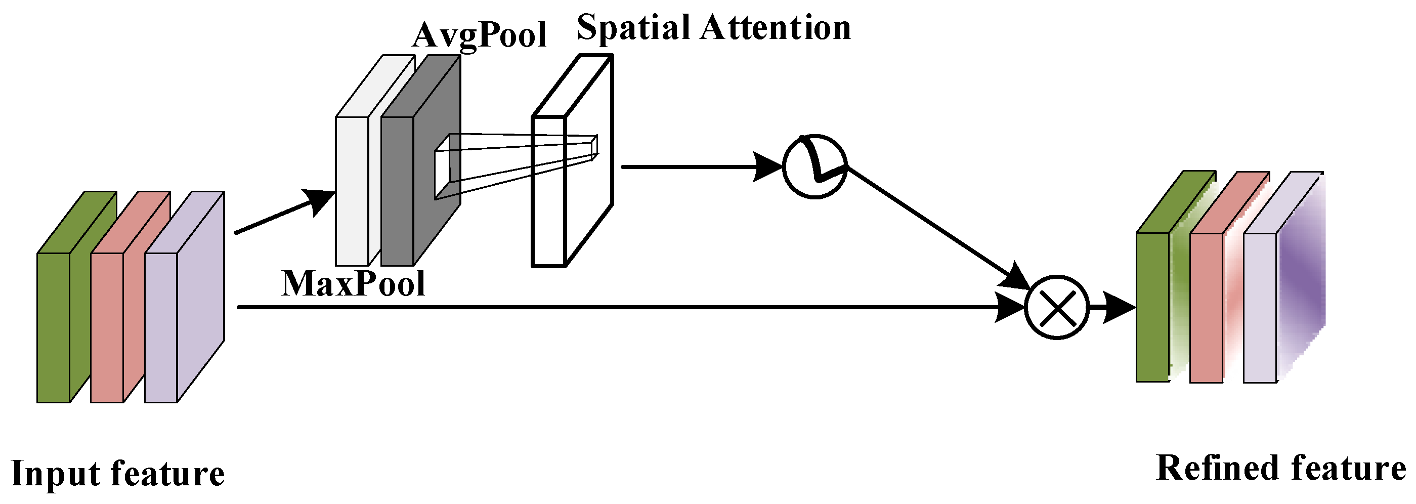
4.2.2. Spatial Attention Module

The module showed in Figure 6 is designed to learn the correlations between different spatial positions [29]. It reshapes the feature map along the channel dimension into a two-dimensional matrix. Then, by passing through a convolutional layer and an activation function, spatial weights are generated. Finally, by multiplying the spatial weights with the feature map, a new feature map is obtained.

In convolutional neural networks, features from different channels and spatial positions have varying importance for different tasks. For instance, in image classification tasks, features from different colour channels have varying abilities to distinguish between different categories. In image segmentation tasks, features from different positions have different capabilities for dividing different regions [30]. Similarly, in the time series regression problem of continuous blood pressure estimation, signals from different channels such as PPG [31], its derivative PPG’, and PPG’’ have different degrees of correlation with blood pressure. The channel attention module can be used to adjust their respective weights. As the values at specific time steps in dynamic blood pressure signals, SBP and DBP also have varying degrees of correlation with the amplitudes of PPG, PPG’, and PPG’’ at different time steps [32]. The time dimension can be viewed as a spatial dimension, and the spatial attention module can be used to weigh signals at different time steps. By adaptively adjusting the feature weights of different channels and time positions, the expressive ability of the model can be improved, resulting in higher accuracy of the final blood pressure estimation.

5. Results

5.1. Experimental Setup

The experiment was conducted on a Windows 10 operating system, utilising Python 3.8 as the primary programming language. To construct and train the TCN-CBAM model, the PyTorch 13.1 deep learning framework was chosen. Additionally, NumPy 2.0 was selected for efficient numerical computations, Pandas 2.0.0 for data manipulation and analysis, Matplotlib 3.4.3 for creating visualisations, and Scikit-learn 0.24.2 for implementing machine learning algorithms. For ease of development and debugging, the versatile and user-friendly Jupyter Notebook served as our main development environment.

The hardware setup for the experiment boasted a high-performance Intel Core i9 processor (Intel, Santa Clara, CA, USA), ensuring swift responsiveness when handling substantial data volumes. Furthermore, to expedite the training and inference processes of the model, an NVIDIA GeForce 4070Ti graphics card (Nvidia, Santa Clara, CA, USA), equipped with adequate CUDA cores and memory, was utilised.

The TCN-CBAM model developed in this study comprises an input layer, four stacked dilated causal convolutional residual blocks, a CBAM attention module, two fully connected layers, and an output layer, as illustrated in the accompanying diagram. The essential hyperparameters for each component are detailed in

Table 1. Comparison of model test results’ accuracy.

Function Block	Hyperparameter
Input layer	size: 3 × 1000
Dilated causal convolution residual block	Convolutional layer	Kernel size: 1 × 3
		Number of kernels: 64
		Dilation factor: 2i
	Normalization layer	Method: batch normalization
	Activation layer	Activation function: ReLU
	Dropout layer	Dropout rate: 0.05%
CBAM attention module	Channel attention layer	Feature reduction rate: 16
	Spatial attention layer	Kernel size: 1 × 7
Fully connected layer	First layer	Input dimensions: 64
		Output dimensions: 128
	Second layer	Input dimensions: 128
		Output dimensions: 1
Output Layer	Output size: 2 × 1

.

During the training process, the Adam optimizer was selected for updating the model parameters. Adam is an optimization algorithm that features adaptive learning rates. It adjusts the learning rates of the model parameters by computing the first-order moments (mean) and the second-order moments (uncentered variance) of the gradients. In each iteration, Adam employs gradient information alongside historically accumulated variables to revise the momentum and the adaptive learning rate of the parameters, incorporating bias correction. Ultimately, the corrected momentum and adaptive learning rate are used to determine the parameter updates, thereby optimizing the model’s weights and biases. During the experimentation, an initial learning rate of 0.0001 was set for the model, with a training batch size of 32 and a total of 1500 iterations.

5.2. Evaluation Metrics and Loss Functions

In the testing of blood pressure estimation models, multiple evaluation metrics are typically chosen to assess the model’s performance comprehensively. In this chapter, we selected mean absolute error (MAE), standard deviation (STD), and mean absolute percentage error (MAPE) as our evaluation metrics. These metrics aid in understanding the model’s prediction accuracy, stability, and percentage error.

(1)

Mean Absolute Error

Mean absolute error calculates the average of the absolute differences between the predicted and actual values [33]. It reflects the overall prediction accuracy of the model. The formula for calculating MAE is as follows:

$$MAE=\frac{1}{n}{\sum }_{i=1}^n{|y}_i-{\widehat{y}}_i|$$

(3)

In the formula, y_i represents the actual blood pressure value, ${\widehat{y}}_i$ represents the blood pressure value predicted by the model, and n represents the sample size. A smaller MAE value indicates more accurate predictions made by the model.

(2)

Standard Deviation

In the context of blood pressure estimation models, standard deviation is typically used to measure the variability of prediction errors [34], indicating the stability of the model’s predictions. The formula for calculating STD is as follows:

$$STD=\sqrt{\frac{1}{n}{\sum }_{i=1}^n{{(y}_i-{\widehat{y}}_i-ME)}^2}$$

(4)

where ME represents the mean error of prediction errors, and its calculation formula is as follows:

$$ME=\frac{1}{n}{\sum }_{i=1}^n{(y}_i-{\widehat{y}}_i)$$

(5)

(3)

Mean Absolute Percentage Error

Mean absolute percentage error (MAPE) measures the average percentage error between the predicted values of the model and the actual values [35]. It provides an understanding of the magnitude of prediction errors relative to the actual values. The formula for calculating MAPE is as follows:

$$MAPE=\frac{1}{n}\sum _{i=1}^n\left|\frac{y_i-{\widehat{y}}_i}{y_i}\right|\times 100\%$$

(6)

When there are zeros or values very close to zero in the actual values y_i, MAPE may become extremely large or impossible to calculate. Therefore, when using MAPE as an evaluation metric, special attention needs to be paid to the characteristics of the dataset. A smaller MAPE value indicates a lower percentage of prediction errors made by the model, suggesting better model performance.

In the experiments of this chapter, MSE was chosen as the loss function during model training. The MSE loss function is one of the commonly used loss functions in regression problems, which measures the difference between the predicted values of the model and the actual values. The calculation formula for the MSE loss function is as follows:

$$MSE=\frac{1}{n}{\sum }_{i=1}^n{{(BP}_i-{\widehat{BP}}_i)}^2$$

(7)

where BP_i represents the actual blood pressure value, ${\widehat{BP}}_i$ represents the blood pressure value predicted by the model, and n represents the sample size, which is the number of samples in the dataset used for training. MSE calculates the average of the squared differences between the predicted values of the model and the actual values. The squaring operation gives larger errors more weight in the loss function, encouraging the model to pay more attention to predictions that deviate further from the actual values. The average ensures that the loss function is comparable across different sample sizes.

5.3. Comparison and Analysis of Experimental Results

The data for this experiment originates from the dataset obtained after preprocessing in Section 3.3. It is divided into a 7:1:2 ratio, with the first 70% serving as the training set, the subsequent 10% as the validation set, and the remaining 20% as the test set. Initially, the TCN-CBAM blood pressure estimation model is thoroughly trained using the training and validation sets until it reaches convergence. Subsequently, PPG data from the test set are inputted into the model to derive the corresponding estimated SBP and DBP values. Based on these estimated values and the actual values (specifically, the SBP and DBP from the test set labels), scatter plots and Bland–Altman plots are generated for analysis. The outcomes are illustrated in Figure 7.

As evident from Figure 7, in the scatter plots of the experimental results for both SBP and DBP, a large number of data points are tightly clustered around the regression lines, each forming a distinct trend line. After conducting Pearson correlation analysis between the model-estimated blood pressure and the reference blood pressure indicated in the label, the Pearson coefficient for the model’s SBP estimate compared to the reference SBP is 0.8; moreover, the model’s DBP estimate, compared to the reference DBP, is 0.6. This indicates a strong positive correlation between the model’s estimated values and the actual measurements. Compared to SBP, the regression line for DBP estimation exhibits a slope closer to 1 and a smaller absolute value for the intercept, suggesting higher overall accuracy. Additionally, the tight distribution of scatter points demonstrates the model’s high degree of generalization when processing blood pressure data from diverse individuals, accurately capturing the nuances of blood pressure variations.

We assessed the performance of the TCN-CBAM model in blood pressure estimation tasks using the BHS standard by analyzing the estimation errors in the test set. The comparison between the error distribution and the BHS criteria is presented in

Table 2. Comparison of TCN-CBAM model test results’ accuracy.

		≤5 mmHg	≤10 mmHg	≤15 mmHg
BHS	Grade A	60%	85%	95%
	Grade B	50%	75%	90%
	Grade C	40%	65%	85%
TCN-CBAM Model test results	SBP Estimation error	48.74%	73.19%	87.06%
	DBP Estimation error	38.62%	88.73%	97.29%

.

To verify the effectiveness of the TCN-CBAM beat-by-beat blood pressure estimation model proposed in this chapter, we selected ten machine learning models for comparison. Six of these are commonly used regression models in machine learning, namely, linear regression, support vector regression (SVR), multilayer perceptron (MLP), XGBoost (XGB), random forest (RF), and K-nearest neighbours regression (KNN). All six models are implemented using the sklearn machine learning library. The other three are deep learning models previously used in continuous blood pressure estimation studies: CNN, CNN-GRU, and CNN-LSTM. The number and size of convolutional kernels used in the CNN models are consistent with those in the TCN-CBAM model. The CNN-GRU model incorporates a two-layer GRU with 128 hidden nodes, while the CNN-LSTM model includes a two-layer LSTM with the same number of hidden nodes.

The error distribution of the estimation results from the eleven aforementioned models is depicted in Figure 8. As evident from the figure, whether for SBP or DBP estimation, the estimation accuracy of the three structurally simpler machine learning models—linear, SVR, and MLP—significantly lags behind that of ensemble learning and deep learning models. While the ensemble learning models, specifically random forest and XGBoost, exhibit noticeable improvement in terms of error reduction, they still trail behind neural network architectures based on CNN and RNN.

The MAE, STD, and MAPE of all the aforementioned models on the test set are shown in

Table 3. Comparison of model test results’ accuracy.

Model	SBP Estimation Error			DBP Estimation Error
	MAE	STD	MAPE	MAE	STD	MAPE
Linear	14.0665	17.9088	0.1097	4.5460	5.8711	0.0653
SVR	12.7897	16.3983	0.0990	4.5311	5.9229	0.0591
MLP	13.5818	17.3121	0.1039	4.3163	5.9181	0.0623
XGBoost	8.4072	11.9345	0.0656	2.9859	4.1835	0.0431
RF	7.1597	10.8400	0.0560	2.7073	3.9852	0.0391
KNN	7.3237	11.1455	0.0569	2.6817	4.0246	0.0386
CNN	8.2555	11.6321	0.0629	3.3077	4.3385	0.0336
CNN-GRU	5.6089	9.1172	0.0431	2.5339	3.7756	0.0368
CNN-LSTM	5.3837	9.0737	0.0420	2.5029	3.7069	0.0361
TCN	5.8680	8.8940	0.0405	2.3707	3.8023	0.0307
TCN-CBAM	5.3482	8.3410	0.0334	2.1190	3.1795	0.0240

.

From the table, it is evident that the proposed TCN-CBAM model in this chapter yielded the best results in both SBP and DBP estimation tasks. For SBP estimation, the MAE, STD, and MAPE stood at 5.3482 mmHg, 8.3410 mmHg, and 3.34%, respectively. While these are respectable figures, they still fall slightly short of the AAMI standard of 5 ± 8 mmHg. In DBP estimation, however, the TCN-CBAM model excelled with metrics of 2.1190 mmHg, 3.1795 mmHg, and 2.40%, meeting the stringent requirements set by the AAMI standard. Notably, the TCN_CBAM model’s MAE, STD, and MAPE were notably lower than its counterparts. This underscores the model’s high precision and stability in blood pressure estimation, effectively tackling intricate blood pressure data and pinpointing crucial features.

Furthermore, deep learning models like CNN-LSTM, CNN-GRU, and TCN showcased commendable performance. These models are inherently adept at handling time-series data, readily capturing long-term dependencies and intricate patterns within the dataset. Consequently, they fared well in blood pressure estimation tasks. In contrast, while traditional machine learning models like XGBoost, RF, and KNN had a decent performance, they lagged behind their deep learning counterparts. This disparity could stem from the limitations of traditional models in navigating complex nonlinear relationships. Nonetheless, these models might still prove useful in specific contexts. The linear model, however, fared the worst in our experiment, likely due to its inability to grasp the intricate nonlinear relationships inherent in blood pressure data.

6. Conclusions

In this paper, we introduce a cuff-less, beat-by-beat blood pressure estimation model, which combines temporal convolutional networks (TCNs) with attention mechanisms. We have modified the standard TCN framework by integrating a CBAM, which allows the model to better identify and focus on critical features, thereby enhancing the precision of blood pressure estimations. We validated our model on a large-scale, publicly available dataset of physiological signals. Specifically, on the UCI physiological signal dataset, our model achieved an absolute mean error and standard deviation of 5.3482 mmHg and 8.3410 mmHg, respectively, for systolic blood pressure estimation. For diastolic blood pressure estimation, the model recorded an absolute mean error and standard deviation of 2.1190 mmHg and 3.1795 mmHg, respectively. These results surpass those obtained using other deep learning models, which are rooted in convolutional neural networks and recurrent neural networks. Our findings confirm that the proposed model significantly outperforms 10 comparative models in beat-by-beat blood pressure estimation tasks. Moreover, our study underscores the superiority of the TCN architecture over CNN, RNN, and hybrid CNN-RNN structures in tackling time series challenges. To further enhance the model’s performance, potential improvements could involve exploring more sophisticated attention mechanisms tailored specifically for physiological time series data, as well as investigating the integration of additional biometric parameters to enrich the feature space. Future research may also include the application of this model to real-time blood pressure monitoring systems, evaluating its performance on diverse populations and refining the model to handle noisy or irregularly sampled data, thereby increasing its robustness and generalizability in clinical settings.

References

1. Progn, V. Hypertension as a Medical and Social Problem and Ways to Solve it. Doctoral Dissertation, Scientific Repository of I.Horbachevsky Ternopil National Medical University, Ternopil, Ukraine, 2022. [Google Scholar]
2. Picone, D.S.; Schultz, M.G.; Otahal, P.; Aakhus, S.; Al-Jumaily, A.M.; Black, J.A.; Bos, W.J.; Chambers, J.B.; Chen, C.H.; Cheng, H.M.; et al. Accuracy of cuff-measured blood pressure: Systematic reviews and meta-analyses. J. Am. Coll. Cardiol. 2017, 70, 572–586. [Google Scholar] [CrossRef]
3. Corazza, I.; Zecchi, M.; Corsini, A.; Marcelli, E.; Cercenelli, L. Technologies for Hemodynamic Measurements: Past, Present and Future. In Advances in Cardiovascular Technology; Academic Press: Cambridge, MA, USA, 2022; pp. 515–566. [Google Scholar]
4. El-Hajj, C.; Kyriacou, P.A. A review of machine learning techniques in photoplethysmography for the non-invasive cuff-less measurement of blood pressure. Biomed. Signal Process. Control 2020, 58, 101870. [Google Scholar] [CrossRef]
5. Vidhya, C.M.; Maithani, Y.; Singh, J.P. Recent advances and challenges in textile electrodes for wearable biopotential signal monitoring: A comprehensive review. Biosensors 2023, 13, 679. [Google Scholar] [CrossRef] [PubMed]
6. Rastegar, S.; GholamHosseini, H.; Lowe, A. Non-invasive continuous blood pressure monitoring systems: Current and proposed technology issues and challenges. Phys. Eng. Sci. Med. 2020, 43, 11–28. [Google Scholar] [CrossRef]
7. Teng, X. Noninvasive and Cuffless Blood Pressure Measurement: The Effects of Contacting Force and Dynamic Exercise; The Chinese University of Hong Kong: Hong Kong, China, 2004. [Google Scholar]
8. Kurylyak, Y.; Lamonaca, F.; Grimaldi, D. A Neural Network-based method for continuous blood pressure estimation from a PPG signal. In Proceedings of the 2013 IEEE International Instrumentation and Measurement Technology Conference (I2MTC), Minneapolis, MN, USA, 6–9 May 2013; IEEE: Piscataway, NJ, USA, 2013; pp. 280–283. [Google Scholar]
9. Liu, M.; Po, L.M.; Fu, H. Cuffless blood pressure estimation based on photoplethysmography signal and its second derivative. Int. J. Comput. Theory Eng. 2017, 9, 202. [Google Scholar] [CrossRef]
10. Maqsood, S.; Xu, S.; Springer, M.; Mohawesh, R. A benchmark study of machine learning for analysis of signal feature extraction techniques for blood pressure estimation using photoplethysmography (PPG). IEEE Access 2021, 9, 138817–138833. [Google Scholar] [CrossRef]
11. Baek, S.; Jang, J.; Yoon, S. End-to-end blood pressure prediction via fully convolutional networks. IEEE Access 2019, 7, 185458–185468. [Google Scholar] [CrossRef]
12. Su, P.; Ding, X.R.; Zhang, Y.T.; Liu, J.; Miao, F.; Zhao, N. Long-term blood pressure prediction with deep recurrent neural networks. In Proceedings of the 2018 IEEE EMBS International Conference on Biomedical & Health Informatics (BHI), Las Vegas, NV, USA, 4–7 March 2018; IEEE: Piscataway, NJ, USA, 2018; pp. 323–328. [Google Scholar]
13. Slapničar, G.; Mlakar, N.; Luštrek, M. Blood pressure estimation from photoplethysmogram using a spectro-temporal deep neural network. Sensors 2019, 19, 3420. [Google Scholar] [CrossRef]
14. Schrumpf, F.; Frenzel, P.; Aust, C.; Osterhoff, G.; Fuchs, M. Assessment of non-invasive blood pressure prediction from ppg and rppg signals using deep learning. Sensors 2021, 21, 6022. [Google Scholar] [CrossRef] [PubMed]
15. White, W.B.; Berson, A.S.; Robbins, C.; Jamieson, M.J.; Prisant, L.M.; Roccella, E.; Sheps, S.G. National standard for measurement of resting and ambulatory blood pressures with automated sphygmomanometers. Hypertension 1993, 21, 504–509. [Google Scholar] [CrossRef]
16. Barna, I.; Keszei, A.; Dunai, A. Evaluation of Meditech ABPM-04 ambulatory blood pressure measuring device, according to the British Hypertension Society (BHS) protocol. Blood Press. Monit. 1998, 3, 363–368. [Google Scholar] [PubMed]
17. Kachuee, M.; Kiani, M.M.; Mohammadzade, H.; Shabany, M. Cuff-less high-accuracy calibration-free blood pressure estimation using pulse transit time. In Proceedings of the 2015 IEEE International Symposium on Circuits and Systems (ISCAS), Lisbon, Portugal, 24–27 May 2015; IEEE: Piscataway, NJ, USA, 2015; pp. 1006–1009. [Google Scholar]
18. Dragomiretskiy, K.; Zosso, D. Variational mode decomposition. IEEE Trans. Signal Process. 2013, 62, 531–544. [Google Scholar] [CrossRef]
19. Knai, K. Oscillations in Biological Signal. Doctoral Thesis, NTNU, Trondheim, Norway, 2020. [Google Scholar]
20. Zhong, X.S. Research on Human Motion Partition Wall Detection and Localization Technology Based on UHF; North Central University: Minneapolis, MN, USA, 2021. [Google Scholar]
21. Cheng, C.; Zhang, C.; Wei, Y.; Jiang, Y.G. Sparse temporal causal convolution for efficient action modeling. In Proceedings of the 27th ACM International Conference on Multimedia, Nice, France, 21–25 October 2019; pp. 592–600. [Google Scholar]
22. Zhang, X.; You, J. A gated dilated causal convolution based encoder-decoder for network traffic forecasting. IEEE Access 2020, 8, 6087–6097. [Google Scholar] [CrossRef]
23. Ma, H.; Chen, C.; Zhu, Q.; Yuan, H.; Chen, L.; Shu, M. An ECG signal classification method based on dilated causal convolution. Comput. Math. Methods Med. 2021, 2021, 6627939. [Google Scholar] [CrossRef] [PubMed]
24. Hamad, R.A.; Kimura, M.; Yang, L.; Woo, W.L.; Wei, B. Dilated causal convolution with multi-head self attention for sensor human activity recognition. Neural Comput. Appl. 2021, 33, 13705–13722. [Google Scholar] [CrossRef]
25. Sherstinsky, A. Fundamentals of recurrent neural network (RNN) and long short-term memory (LSTM) network. Phys. D Nonlinear Phenom. 2020, 404, 132306. [Google Scholar] [CrossRef]
26. Woo, S.; Park, J.; Lee, J.Y.; Kweon, I.S. Cbam: Convolutional block attention module. In Proceedings of the European Conference on Computer Vision (ECCV), Munich, Germany, 8–14 September 2018; pp. 3–19. [Google Scholar]
27. Yang, J.; Jiang, J. Dilated-CBAM: An efficient attention network with dilated convolution. In Proceedings of the 2021 IEEE International Conference on Unmanned Systems (ICUS), Beijing, China, 15–17 October 2021; IEEE: Piscataway, NJ, USA, 2021; pp. 11–15. [Google Scholar]
28. Chen, B.; Dang, Z. Fast PCB defect detection method based on FasterNet backbone network and CBAM attention mechanism integrated with feature fusion module in improved YOLOv7. IEEE Access 2023, 11, 95092–95103. [Google Scholar] [CrossRef]
29. Zhu, X.; Cheng, D.; Zhang, Z.; Lin, S.; Dai, J. An empirical study of spatial attention mechanisms in deep networks. In Proceedings of the IEEE/CVF International Conference on Computer Vision, Seoul, South Korea, 27 October–2 November 2019; pp. 6688–6697. [Google Scholar]
30. Chen, B.; Huang, Y.; Xia, Q.; Zhang, Q. Nonlocal spatial attention module for image classification. Int. J. Adv. Robot. Syst. 2020, 17, 1729881420938927. [Google Scholar] [CrossRef]
31. Hu, M.; Guo, D.; Jiang, M.; Qian, F.; Wang, X.; Ren, F. rPPG-based heart rate estimation using spatial-temporal attention network. IEEE Trans. Cogn. Dev. Syst. 2021, 14, 1630–1641. [Google Scholar] [CrossRef]
32. Kim, S.C. Analysis of Change Rate of SBP and DBP Estimation Fusion Algorithm According to PTT Measurement change PPG Pulse Wave Analysis. J. Korea Converg. Soc. 2020, 11, 35–40. [Google Scholar]
33. Chai, T.; Draxler, R.R. Root mean square error (RMSE) or mean absolute error (MAE). Geosci. Model Dev. Discuss. 2014, 7, 1525–1534. [Google Scholar]
34. Lee, D.K.; In, J.; Lee, S. Standard deviation and standard error of the mean. Korean J. Anesthesiol. 2015, 68, 220. [Google Scholar] [CrossRef] [PubMed]
35. De Myttenaere, A.; Golden, B.; Le Grand, B.; Rossi, F. Mean absolute percentage error for regression models. Neurocomputing 2016, 192, 38–48. [Google Scholar] [CrossRef]
Figure 1. The processing result of the PPG signal is processed using the VMD algorithm.
Applsci 14 06061 g001
Figure 2. Dataset label distribution: (a) training set; (b) test set.
Applsci 14 06061 g002
Figure 3. TCN-CBAM network architecture.
Applsci 14 06061 g003
Figure 4. Dilated causal convolution.
Applsci 14 06061 g004
Figure 5. Channel attention module.
Applsci 14 06061 g005
Figure 6. Spatial attention module.
Applsci 14 06061 g006
Figure 7. Scatter plot and Bland–Altman plot of model test results: (a) SBP, (b) DBP.
Applsci 14 06061 g007
Figure 8. Error distribution of estimation results from different models.
Applsci 14 06061 g008